Open Journal of Mathematical Sciences
Vol. 6 (2022), Issue 1, pp. 269 – 280
ISSN: 2523-0212 (Online) 2616-4906 (Print)
DOI: 10.30538/oms2022.0192

Application of the newly \(\varphi^{6}\)-model expansion approach to the nonlinear reaction-diffusion equation

Muhammad Abubakar Isah\(^{1,*}\) and Asif Yokus\(^{1}\)
\(^{1}\) Department of Mathematics, Faculty of Science, Firat University, Elazig, Turkey.
Correspondence should be addressed to Muhammad Abubakar Isah at myphysics_09@hotmail.com

Copyright © 2022 Muhammad Abubakar Isah and Asif Yokus. This is an open access article distributed under the Creative Commons Attribution License, which permits unrestricted use, distribution, and reproduction in any medium, provided the original work is properly cited.

Received: June 30, 2022 – Accepted: October 21, 2022 – Published: December 31, 2022

Abstract

In this paper, we use the \(\varphi ^{6}\)-model expansion method to construct the traveling wave solutions for the reaction-diffusion equation. The method of \(\varphi ^{6}\)-model expansion enables the explicit retrieval of a wide variety of solution types, such as bright, singular, periodic, and combined singular soliton solutions. Kink-type solitons, also known as topological solitons in the context of water waves, are another type of solution that can be explicitly retrieved. This study’s results might enhance the equation’s nonlinear dynamical properties. The method proposes a practical and efficient method for solving a sizable class of nonlinear partial differential equations. The dynamical features of the data are explained and highlighted using exciting graphs.

Keywords:

Reaction-diffusion equation; \(\varphi ^{6}\)-model expansion method; Soliton solutions; Kink soliton.

1. Introduction

The study of surfaces in geometry (see [1,2,3,4,5]) and a variety of mechanical issues are where partial differential equations (PDEs) first showed up. The study of various issues brought on by partial differential equations attracted the attention of eminent mathematicians worldwide in the late 19th century. This work was primarily motivated by the fact that partial differential equations commonly appear in the mathematical analysis of a wide range of problems in science and engineering and describe many fundamental natural laws [6]. It is now incredibly beneficial to look for precise answers to nonlinear evolution equations and partial differential equations NLEEs using various techniques. There are numerous effective techniques, such as the inverse scattering transform approach [7], the Homoclinic technique [8], the sinh-Gordon function method [9], the generalized exponential rational function method [10], the auxiliary equation method [11], An alternative method [12], the Bernoulli sub-equation function method [13,14], the sub-equation analytical method [15], the modified sub-equation method [16], the auto-Backlund transformation method [17] and so on.

This study focuses on the reaction-diffusion equation, and the equation has been investigated via many direct methods. Among these are; The sine-Gordon expansion method [18], the rational \((G'/G)\)-expansion method [19], the \((G'/G)\)-expansion method [20], the projective Riccati equation method [21]. The reaction-diffusion model is studied in this research using the newly developed \(\varphi ^{6}\)--model expansion method [22,23,24,25]), which results in the restoration of optical solitary wave solutions.

The plan for this work is provided below. In §2, a presentation of the \(\varphi ^{6}\)-model expansion method will be provided. Next, the reaction-diffusion model will be developed using the \(\varphi 6\) approach in §3 to provide new traveling wave solutions to the reaction-diffusion equation. Moreover, the associated 3D, 2D, and density graphs clearly illustrate the physical structure of the traveling wave solution. Finally, in §4, conclusions are reached.

2. The \(\varphi ^{6}\)-model expansion technique

According to [22,23,24,25], the steps involves for the \(\varphi ^{6}\)-model expansion technique are given as:

Step-1: Assuming the nonlinear evolution equation (NLEE) for \(W=W(x,t)\) is in the form.

\begin{equation} H(W,W_{x},W_{t},W_{xx},W_{xt},...)=0, \label{9} \end{equation}

(1)

here \(H\) is a polynomial of \(W(x,t)\) which involves highest order partial derivatives and its nonlinear terms.

Step-2: By using the wave transformation

\begin{equation} W(x,t)=W(\zeta ), \zeta =x - vt, \label{10} \end{equation}

(2)

where \(v\) represents wave speed and Eq. (1) can be converted into the nonlinear ordinary differential equation shown below.

\begin{equation} \Omega (W,W^{^{\prime }},WW^{^{\prime }},W^{^{\prime \prime }},...)=0, \label{11} \end{equation}

(3)

where the derivatives with respect to \(\zeta \) are shown by prime.

Step-3: Suppose that the formal solution to Eq. (3) exists:

\begin{equation} W\left( \zeta \right) =\sum\limits_{j=0}^{2M}\alpha _{j}Q^{j}(\zeta ), \label{12} \end{equation}

(4)

\(M\) can be gotten using the balancing rule, \(\alpha _{j}(j=0,1,2, \ldots ,M)\) are to be determined constants and \(Q(\zeta )\) satisfies the auxiliary NLODE;

\begin{equation}\label{13} \begin{cases} Q^{\prime 2}(\zeta )=h_{0}+h_{2}Q^{2}(\zeta )+h_{4}Q^{4}(\zeta )+h_{6}Q^{6}(\zeta ), \\ Q^{^{\prime \prime }}(\zeta ) =h^{2}Q(\zeta )+2h_{4}Q^{3}(\zeta )+3h_{6}Q^{5}(\zeta ), \end{cases}\end{equation}

(5)

here \(h_{j}(j=0,2,4,6)\) are real constants that will be found later.

Step-4: It is known that the solution to Eq. (5) is given as;

\begin{equation} Q(\zeta )=\frac{P(\zeta )}{\sqrt{fP^{2}(\zeta )+g}}, \label{14} \end{equation}

(6)

\(P(\zeta )\) is the Jacobi elliptic equation solution, provided that \(0< fP^{2}(\zeta )+g\)

\begin{equation} P^{\prime 2}(\zeta )=l_{0}+l_{2}P^{2}(\zeta )+l_{4}P^{4}(\zeta ), \label{15} \end{equation}

(7)

where \(l_{j}(j=0,2,4)\) are unknown constants to be determined, \(g\) and \(f\) are given by

\begin{equation}\label{16} \begin{cases} f =\frac{h_{4}(l_{2}-h_{2})}{% (l_{2}-h_{2})^{2}+3l_{0}l_{4}-2l_{2}(l_{2}-h_{2})}, \\ g =\frac{3l_{0}h_{4}}{(l_{2}-h_{2})^{2}+3l_{0}l_{4}-2l_{2}(l_{2}-h_{2})}, \end{cases}\end{equation}

(8)

under the restricted condition

\begin{equation} h_{4}^{2}(l_{2}-h_{2})[9l_{0}l_{4}-(l_{2}-h_{2})(2l_{2}+h_{2})]+3h_{6}[-l_{2}^{2}+h_{2}^{2}+3l_{0}l_{4}]^{2}=0. \label{17} \end{equation}

(9)

Step-5: The Jacobi elliptic solutions of Eq. (7) can be calculated when \(0< m< 1\), the exact solutions of Eq. (1) can be derived by substituting Eq. (6) and Eq. (7) into Eq. (4).

Function	\(m\rightarrow 1\)	\(m\rightarrow 0\)	Function	\(m\rightarrow 1\)	\(m\rightarrow 0\)
\(sn(\zeta ,m)\)	\(tanh(\zeta )\)	\(sin(\zeta )\)	\(ds(\zeta ,m)\)	\(csch(\zeta )\)	\(csc(\zeta )\)
\(cn(\zeta ,m)\)	\(sech(\zeta )\)	\(cos(\zeta )\)	\(sc(\zeta ,m)\)	\(sinh(\zeta )\)	\(tan(\zeta )\)
\(dn(\zeta ,m)\)	\(sech(\zeta )\)	\(1\)	\(sd(\zeta ,m)\)	\(sinh(\zeta )\)	\(sin(\zeta )\)
\(ns(\zeta ,m)\)	\(coth(\zeta )\)	\(csc(\zeta )\)	\(nc(\zeta ,m)\)	\(cosh(\zeta )\)	\(sec(\zeta )\)
\(cs(\zeta ,m)\)	\(csch(\zeta )\)	\(cot(\zeta )\)	\(cd(\zeta ,m)\)	\(1\)	\(cos(\zeta )\)

3. Application to the reaction-diffusion equation

The \(\varphi ^{6}\)-model expansion method, which was explained in the previous part, we take into account the reaction-diffusion equation's following form.

\begin{equation} {W_{tt}} + d W + n{W^3} + \beta {W_{xx}} = 0, \label{18} \end{equation}

(10)

here real constants \(\beta\) , \(d\) and \(n\) are the real constants, Eq. (10) is reduced to the following ODE using the traveling wave transformation \(W(x, t) = W(\zeta) = G(x- vt)\):

\begin{equation} {(v^2 + \beta)}{W^{''}} + n{W^3} + d W = 0, \label{19} \end{equation}

(11)

where \(M+2=3M\), therefore, \(M= 1\) is obtained as a result of the balance principle between \({W^{''}}\) and \({W^3}\); so, the solution form can be expressed as

\begin{equation} W(\zeta )=\alpha _{0}+\alpha _{1}Q(\zeta )+\alpha _{2}Q^{2}(\zeta ), \label{21} \end{equation}

(12)

where \(\alpha _{0},\alpha _{1}\) and \(\alpha _{2}\) are constants to be determined.

We obtain the following algebraic equations by substituting Eq. (12) along with Eq. (5) into Eq. (11) and setting the coefficients of all powers of \(Q^{j}(\zeta )\), \(j=0,1,\ldots ,6\) to be equal to zero;

\begin{equation} \begin{cases} {Q^0}(\zeta ): \alpha _0 d+2 \alpha _2 \beta h_0+2 \alpha _2 h_0 v^2+\alpha _0^3 n= 0,\\ {Q^1}(\zeta ): \alpha _1 d+\alpha _1 \beta h_2+\alpha _1 h_2 v^2+3 \alpha _0^2 \alpha _1 n= 0,\\ {Q^2}(\zeta ): \alpha _2 d+4 \alpha _2 \beta h_2+4 \alpha _2 h_2 v^2+3 \alpha _0 \alpha _1^2 n+3 \alpha _0^2 \alpha _2 n= 0,\\ {Q^3}(\zeta ): 2 \alpha _1 \beta h_4+2 \alpha _1 h_4 v^2+\alpha _1^3 n+6 \alpha _0 \alpha _2 \alpha _1 n= 0,\\ {Q^4}(\zeta ): 6 \alpha _2 \beta h_4+6 \alpha _2 h_4 v^2+3 \alpha _0 \alpha _2^2 n+3 \alpha _1^2 \alpha _2 n= 0,\\ {Q^5}(\zeta ): 3 \alpha _1 \beta h_6+3 \alpha _1 h_6 v^2+3 \alpha _1 \alpha _2^2 n= 0,\\ {Q^6}(\zeta ): 8 \alpha _2 \beta h_6+8 \alpha _2 h_6 v^2+\alpha _2^3 n=0. \end{cases} \end{equation}

(13)

The following solutions are obtained after solving the above system of equations:%

\begin{equation}\label{23} \begin{cases} \alpha _0 = 0,\quad {\alpha _1} = \frac{i \sqrt{2} \sqrt{h_4} \sqrt{\beta +v^2}}{\sqrt{n}},\quad \alpha _2=0, \\ d=h_2 \left(-v^2\right)-\beta h_2,\quad {h_6} = 0.\end{cases} \end{equation}

(14)

The following solutions of Eq. (10) can be obtained with the help of Eqs. (6), (12) and (14) along with the Jacobi elliptic functions in the table above.

1. If \(l_{0}=1\), \(l_{2}=-(1+m^{2})\), \(l_{4}=m^{2}\), \(0< m< 1\), then \(% P(\zeta )=sn(\zeta ,m)\) or \(P(\zeta )=cd(\zeta ,m)\), and we have

\begin{equation} W_{_{1,0}}\left( x,t\right) =\alpha _1 \left( \frac{sn(\zeta ,m)}{\sqrt{f\left( sn(\zeta ,m)\right) ^{2}+g}}\right) , \label{24} \end{equation}

(15)

\begin{equation} W_{_{1,1}}\left( x,t\right) =\alpha _1 \left( \frac{cd(\zeta ,m)}{\sqrt{f\left( cd(\zeta ,m)\right) ^{2}+g}}\right), \label{25} \end{equation}

(16)

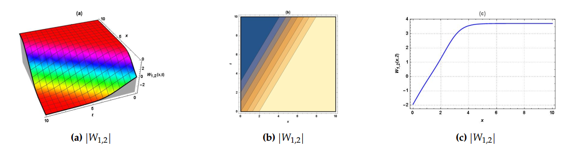
such that \(\zeta =x-vt\) and \(f\) and \(g\) in Eq. (8) are given by \begin{align*} f& =\frac{h_4 \left(h_2+m^2+1\right)}{-h_2^2+m^4-m^2+1}, \\ g& =-\frac{3 h_4}{-h_2^2+m^4-m^2+1}, \end{align*} under the restriction condition \begin{equation*} h_4^2 \left(-h_2-m^2-1\right)\left(9 m^2-\left(-h_2-m^2-1\right) \left(h_2+2 \left(-m^2-1\right)\right)\right) =0. \end{equation*} If \(m\rightarrow 1\), then the kink soliton is obtained

\begin{equation} W_{_{1,2}}\left( x,t\right) =-\frac{i \sqrt{2} \sqrt{h_4} \sqrt{\beta +v^2} \tanh (t v-x)}{\sqrt{n} \sqrt{\frac{h_4 \left(3-\left(h_2+2\right) \tanh ^2(t v-x)\right)}{h_2^2-1}}} , \label{26} \end{equation}

(17)

such that \begin{equation*} h_4^2 \left(-h_2-2\right)\left(9-\left(-h_2-2\right) \left(h_2-4\right)\right) =0. \end{equation*}

Figure 1. The numerical simulations corresponding to \(\left| {{W}_{1,2}} \right|\) given by Eq. (17), for \(m=1\) ; (a) is the 3D graphic, (b) is the 2D-contour graphic while (c) is the 2D graphic for \( \beta=0.1, v =0.6, n = 0.5, h_4=0.3, h_2=0.1 .\)

If \(m\rightarrow 0\), then the periodic solution is obtained

\begin{equation} W_{_{1,3}}\left( x,t\right) =-\frac{i \sqrt{2} \sqrt{h_4} \sqrt{\beta +v^2} \sin (t v-x)}{\sqrt{n} \sqrt{h_4 \left(\frac{3}{h_2^2-1}-\frac{\sin ^2(t v-x)}{h_2-1}\right)}}, \label{27} \end{equation}

(18)

such that \begin{equation*} h_4^2 \left(-h_2-1\right)\left(-\left(-h_2-1\right) \left(h_2-2\right)\right)=0. \end{equation*}

Figure 2. The numerical simulations corresponding to \(\left| {{W}_{1,3}} \right|\) given by Eq. (18), for \(m=1\) ; (a) is the 3D graphic, (b) is the 2D-contour graphic while (c) is the 2D graphic for \( \beta=0.2, v =0.12, n = 0.15, h_4=0.03, h_2=0.1 .\)

2. If \(l_{0}=1-m^{2}\), \(l_{2}=2m^{2}-1\), \(% l_{4}=-m^{2} \), \(0< m< 1\), then \(P(\zeta )=cn(\zeta ,m)\) therefore

\begin{equation} W_{_{2,1}}\left( x,t\right) =\alpha _1 \left( \frac{cn(\zeta ,m)}{\sqrt{f\left( cn(\zeta ,m)\right) ^{2}+g}}\right), \label{28} \end{equation}

(19)

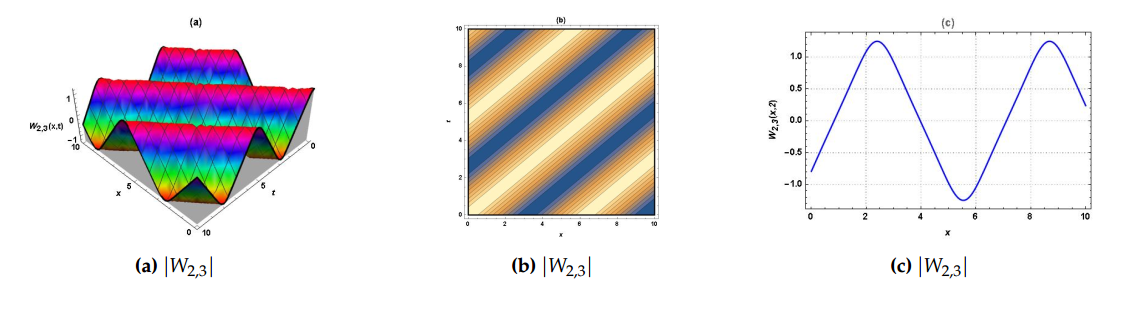
where \(f\) and \(g\) are determined by \begin{align*} f& =\frac{h_4 \left(h_2-2 m^2+1\right)}{-h_2^2+m^4-m^2+1}, \\ g& =\frac{3 h_4 \left(m^2-1\right)}{-h_2^2+m^4-m^2+1}, \end{align*} under the constraint condition \begin{equation*} h_4^2 \left(-h_2+2 m^2-1\right)\left(-\left(-h_2+2 m^2-1\right) \left(h_2+2 \left(2 m^2-1\right)\right)-9 \left(1-m^2\right) m^2\right)=0 \end{equation*} If \(m\rightarrow 1\), then the bright soliton is retrieved

\begin{equation} {{W}_{2,2}}\left( x,t \right)=\frac{i \sqrt{2} \sqrt{h_4} \sqrt{\beta +v^2} \text{sech}(t v-x)}{\sqrt{n} \sqrt{-\frac{h_4 \text{sech}^2(t v-x)}{h_2+1}}} \label{29} \end{equation}

(20)

provided that \begin{equation*} h_4^2 \left(1-h_2\right)\left(-\left(1-h_2\right) \left(h_2+2\right)\right) =0. \end{equation*} If \(m\rightarrow 0\), then the periodic solution is obtained

\begin{equation} W_{_{2,3}}\left( x,t\right) =\frac{i \sqrt{2} \sqrt{h_4} \sqrt{\beta +v^2} \cos (t v-x)}{\sqrt{n} \sqrt{h_4 \left(\frac{3}{h_2^2-1}-\frac{\cos ^2(t v-x)}{h_2-1}\right)}}, \label{30} \end{equation}

(21)

such that \begin{equation*} h_4^2 \left(-h_2-1\right)\left(-\left(-h_2-1\right) \left(h_2-2\right)\right)=0. \end{equation*}

Figure 3. The numerical simulations corresponding to \(\left| {{W}_{2,3}} \right|\) given by Eq. (21), for \(m=1\) ; (a) is the 3D graphic, (b) is the 2D-contour graphic while (c) is the 2D graphic for \( \beta=0.3, v =1.2, n = 1.2, h_4=0.4, h_2=0.3 \).

3. If \(l_{0}=m^{2}-1\), \(l_{2}=2-m^{2}\), \(l_{4}=-1\), \(0< m< 1\), then \(% P(\zeta )=dn(\zeta ,m)\) which gives

\begin{equation} W_{_{3,1}}\left( x,t\right) =\alpha _1 \left( \frac{dn(\zeta ,m)}{\sqrt{f\left( dn(\zeta ,m)\right) ^{2}+g}}\right), \label{31} \end{equation}

(22)

where \(f\) and \(g\) are determined by \begin{align*} f& =\frac{h_4 \left(h_2+m^2-2\right)}{-h_2^2+m^4-m^2+1}, \\ g& =-\frac{3 h_4 \left(m^2-1\right)}{-h_2^2+m^4-m^2+1}, \end{align*} under the restriction condition \begin{equation*} h_4^2 \left(-h_2-m^2+2\right)\left(-\left(-h_2-m^2+2\right) \left(h_2+2 \left(2-m^2\right)\right)-9 \left(m^2-1\right)\right)=0 \end{equation*} If \(m\rightarrow 0\), then the rational solution is obtained

\begin{equation} W_{_{3,3}}\left( x,t\right) =\frac{i \sqrt{2} \sqrt{h_4} \sqrt{\beta +v^2}}{\sqrt{-\frac{\left(h_2-2\right) h_4}{h_2^2-1}-\frac{3 h_4}{h_2^2-1}} \sqrt{n}}, \label{33} \end{equation}

(23)

such that \begin{equation*} h_4^2 \left(2-h_2\right)\left(9-\left(2-h_2\right) \left(h_2+4\right)\right) =0. \end{equation*}

4. If \(l_{0}=m^{2}\), \(l_{2}=-\left( 1+m^{2}\right) \), \(l_{4}=1\), \(% 0< m< 1\), then \(P(\zeta )=ns(\zeta ,m)\) or \(P(\zeta )=dc(\zeta ,m)\) then

\begin{equation} W_{_{4,0}}\left( x,t\right) =\alpha _1 \left( \frac{ns(\zeta ,m)}{\sqrt{f\left( ns(\zeta ,m)\right) ^{2}+g}}\right), \label{34} \end{equation}

(24)

\begin{equation} W_{_{4,1}}\left( x,t\right) =\alpha _1 \left( \frac{dc(\zeta ,m)}{\sqrt{f\left( dc(\zeta ,m)\right) ^{2}+g}}\right), \label{35} \end{equation}

(25)

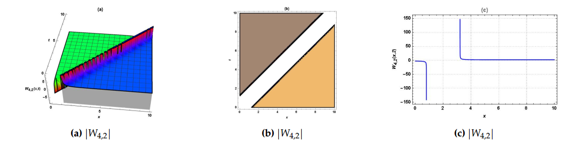
where \(f\) and \(g\) are given by \begin{align*} f& =\frac{h_4 \left(h_2+m^2+1\right)}{-h_2^2+m^4-m^2+1}, \\ g& =-\frac{3 h_4 m^2}{-h_2^2+m^4-m^2+1}, \end{align*} under the constraint condition \begin{equation*} h_4^2 \left(-h_2-m^2-1\right)\left(9 m^2-\left(-h_2-m^2-1\right) \left(h_2+2 \left(-m^2-1\right)\right)\right) =0. \end{equation*} If \(m\rightarrow 1\), then the dark singular solution is obtained

\begin{equation} {{W}_{4,2}}\left( x,t \right)=-\frac{i \sqrt{2} \sqrt{h_4} \sqrt{\beta +v^2} \coth (t v-x)}{\sqrt{n} \sqrt{-\frac{h_4 \left(\left(h_2+2\right) \text{csch}^2(t v-x)+h_2-1\right)}{h_2^2-1}}} \label{36} \end{equation}

(26)

such that \begin{equation*} h_4^2 \left(-h_2-2\right)\left(9-\left(-h_2-2\right) \left(h_2-4\right)\right) =0 \end{equation*}

Figure 4. The numerical simulations corresponding to \(\left| {{W}_{4,2}} \right|\) given by Eq. (26), for \(m=1\) ; (a) is the 3D graphic, (b) is the 2D-contour graphic while (c) is the 2D graphic for \( \beta=3.5, v =1.001, n = 2.1, h_4=0.6, h_2=0.1 \).

If \(m\rightarrow 0\), then the periodic solution is obtained

\begin{equation} W_{_{4,3}}\left( x,t\right) =-\frac{i \sqrt{2} \sqrt{h_4} \sqrt{\beta +v^2} \csc (t v-x)}{\sqrt{n} \sqrt{-\frac{h_4 \csc ^2(t v-x)}{h_2-1}}}, \label{37} \end{equation}

(27)

such that \begin{equation*} h_4^2 \left(-h_2-1\right)\left(-\left(-h_2-1\right) \left(h_2-2\right)\right) =0. \end{equation*}

5. If \(l_{0}=-m^{2}\), \(l_{2}=2m^{2}-1\), \(l_{4}=1-m^{2}\), \(0< m< 1\), then \(P(\zeta )=nc(\zeta ,m)\) and we have

\begin{equation} W_{_{5,1}}\left( x,t\right) =\alpha _1 \left( \frac{nc(\zeta ,m)}{\sqrt{f\left( nc(\zeta ,m)\right) ^{2}+g}}\right), \label{38} \end{equation}

(28)

where \(f\) and \(g\) are given by \begin{align*} f& =\frac{h_4 \left(h_2-2 m^2+1\right)}{-h_2^2+m^4-m^2+1}, \\ g& =\frac{3 h_4 m^2}{-h_2^2+m^4-m^2+1}, \end{align*} under the constraint condition \begin{equation*} h_4^2 \left(-h_2+2 m^2-1\right)\left(-\left(-h_2+2 m^2-1\right) \left(h_2+2 \left(2 m^2-1\right)\right)-9 \left(1-m^2\right) m^2\right) =0. \end{equation*} If \(m\rightarrow 1\), then the singular solitary wave solution is obtained

\begin{equation} W_{_{5,2}}\left( x,t\right) =\frac{i \sqrt{2} \sqrt{h_4} \sqrt{\beta +v^2} \cosh (t v-x)}{\sqrt{n} \sqrt{h_4 \left(-\frac{\cosh ^2(t v-x)}{h_2+1}-\frac{3}{h_2^2-1}\right)}}, \label{39} \end{equation}

(29)

such that \begin{equation*} h_4^2 \left(1-h_2\right)\left(-\left(1-h_2\right) \left(h_2+2\right)\right)=0. \end{equation*}

Figure 5. The numerical simulations corresponding to \(\left| {{W}_{5,2}} \right|\) given by Eq. (29), for \(m=1\) ; (a) is the 3D graphic, (b) is the 2D-contour graphic while (c) is the 2D graphic for \( \beta=0.9, v =0.75, n = 0.2, h_4=1.8, h_2=0.3 \).

If \(m\rightarrow 0\), then the periodic solution is obtained

\begin{equation} W_{_{5,3}}\left( x,t\right) =\frac{i \sqrt{2} \sqrt{h_4} \sqrt{\beta +v^2} \sec (t v-x)}{\sqrt{n} \sqrt{-\frac{h_4 \sec ^2(t v-x)}{h_2-1}}}, \label{40} \end{equation}

(30)

such that \begin{equation*} h_4^2 \left(-h_2-1\right)\left(-\left(-h_2-1\right) \left(h_2-2\right)\right) =0. \end{equation*}

6. If \(l_{0}=-1\), \(l_{2}=2-m^{2}\), \(l_{4}=-\left( 1-m^{2}\right) \), \(0< m< 1\), then \(P(\zeta )=nd(\zeta ,m)\) and we have

\begin{equation} W_{_{6}}\left( x,t\right) =\alpha _1 \left( \frac{nd(\zeta ,m)}{\sqrt{f\left( nd(\zeta ,m)\right) ^{2}+g}}\right), \label{41} \end{equation}

(31)

where \(f\) and \(g\) are given by \begin{align*} f& =\frac{h_4 \left(h_2+m^2-2\right)}{-h_2^2+m^4-m^2+1}, \\ g& =\frac{3 h_4}{-h_2^2+m^4-m^2+1}, \end{align*} under the constraint condition \begin{equation*} h_4^2 \left(-h_2-m^2+2\right)\left(-\left(-h_2-m^2+2\right) \left(h_2+2 \left(2-m^2\right)\right)-9 \left(m^2-1\right)\right) =0. \end{equation*}

7. If \(l_{0}=1\), \(l_{2}=2-m^{2}\), \(l_{4}=1-m^{2}\),\(0< m< 1\), then \(P(\zeta )=sc(\zeta ,m)\), and we have

\begin{equation} W_{_{7,1}}\left( x,t\right) =\alpha _1 \left( \frac{sc(\zeta ,m)}{\sqrt{f\left( sc(\zeta ,m)\right) ^{2}+g}}\right), \label{42} \end{equation}

(32)

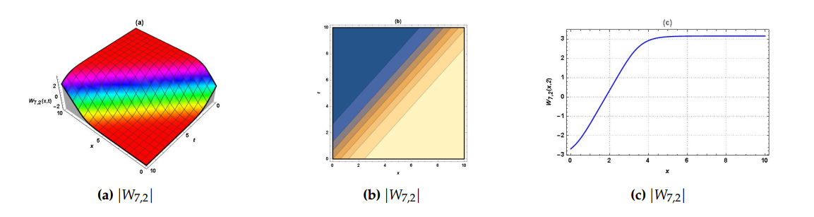
where \(f\) and \(g\) are given by \begin{align*} f& =\frac{h_4 \left(h_2+m^2-2\right)}{-h_2^2+m^4-m^2+1}, \\ g& =-\frac{3 h_4}{-h_2^2+m^4-m^2+1}, \end{align*} under the constraint condition \begin{equation*} h_4^2 \left(-h_2-m^2+2\right)\left(9 \left(1-m^2\right)-\left(-h_2-m^2+2\right) \left(h_2+2 \left(2-m^2\right)\right)\right) =0. \end{equation*} If \(m\rightarrow 1\), then the soliton solution is retrieved

\begin{equation} W_{_{7,2}}\left( x,t\right) =-\frac{i \sqrt{2} \sqrt{h_4} \sqrt{\beta +v^2} \sinh (t v-x)}{\sqrt{n} \sqrt{h_4 \left(\frac{3}{h_2^2-1}-\frac{\sinh ^2(t v-x)}{h_2+1}\right)}}, \label{43} \end{equation}

(33)

such that \begin{equation*} h_4^2 \left(1-h_2\right)\left(-\left(1-h_2\right) \left(h_2+2\right)\right)=0. \end{equation*}

Figure 6. The numerical simulations corresponding to \(\left| {{W}_{7,2}} \right|\) given by Eq. (33), for \(m=1\) ; (a) is the 3D graphic, (b) is the 2D-contour graphic while (c) is the 2D graphic for \( \beta=0.1, v =0.9, n = 0.2, h_4=0.24, h_2=0.1 \).

If \(m\rightarrow 0\), then the periodic wave solution is obtained

\begin{equation} W_{_{7,3}}\left( x,t\right) =-\frac{i \sqrt{2} \sqrt{h_4} \sqrt{\beta +v^2} \tan (t v-x)}{\sqrt{n} \sqrt{\frac{h_4 \left(3-\left(h_2-2\right) \tan ^2(t v-x)\right)}{h_2^2-1}}}, \label{44} \end{equation}

(34)

such that \begin{equation*} h_4^2 \left(2-h_2\right)\left(9-\left(2-h_2\right) \left(h_2+4\right)\right)=0. \end{equation*}

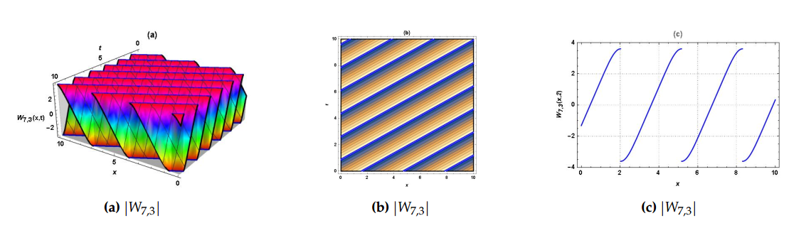
Figure 7. The numerical simulations corresponding to \(\left| {{W}_{7,3}} \right|\) given by Eq. (34), for \(m=1\) ; (a) is the 3D graphic, (b) is the 2D-contour graphic while (c) is the 2D graphic for \( \beta=0.5, v =1.8, n = 0.3, h_4=0.06, h_2=0.1 \).

8. If \(l_{0}=1\), \(l_{2}=2m^{2}-1\), \(l_{4}=-m^{2}\left( 1-m^{2}\right) \), \(0< m< 1\), then \(P(\zeta )=sd(\zeta ,m)\) and we have

\begin{equation} W_{_{8}}\left( x,t\right) =\alpha _1 \left( \frac{sd(\zeta ,m)}{\sqrt{f\left( sd(\zeta ,m)\right) ^{2}+g}}\right), \label{45} \end{equation}

(35)

where \(f\) and \(g\) are given by \begin{align*} f& =\frac{h_4 \left(h_2-2 m^2+1\right)}{-h_2^2+m^4-m^2+1}, \\ g& =-\frac{3 h_4}{-h_2^2+m^4-m^2+1}, \end{align*} under the constraint condition \begin{equation*} h_4^2 \left(-h_2+2 m^2-1\right)\left(-\left(-h_2+2 m^2-1\right) \left(h_2+2 \left(2 m^2-1\right)\right)-9 \left(1-m^2\right) m^2\right) =0. \end{equation*}

9. If \(l_{0}=1-m^{2}\), \(l_{2}=2-m^{2}\), \(l_{4}=1\), \(0< m< 1\), then \(% P(\zeta )=cs(\zeta ,m)\) and we have

\begin{equation} W_{_{9,1}}\left( x,t\right) =\alpha _1 \left( \frac{cs(\zeta ,m)}{\sqrt{f\left( cs(\zeta ,m)\right) ^{2}+g}}\right), \label{46} \end{equation}

(36)

where \(f\) and \(g\) are given by \begin{align*} f& =\frac{h_4 \left(h_2+m^2-2\right)}{-h_2^2+m^4-m^2+1}, \\ g& =\frac{3 h_4 \left(m^2-1\right)}{-h_2^2+m^4-m^2+1}, \end{align*} under the constraint condition \begin{equation*} h_4^2 \left(-h_2-m^2+2\right)\left(9 \left(1-m^2\right)-\left(-h_2-m^2+2\right) \left(h_2+2 \left(2-m^2\right)\right)\right) =0. \end{equation*} If \(m\rightarrow 1\), then the singular soliton solution is obtained

\begin{equation} {{W}_{9,2}}\left( x,t \right)=-\frac{i \sqrt{2} \sqrt{h_4} \sqrt{\beta +v^2} \text{csch}(t v-x)}{\sqrt{n} \sqrt{-\frac{h_4 \text{csch}^2(t v-x)}{h_2+1}}}, \label{47} \end{equation}

(37)

such that \begin{equation*} h_4^2 \left(1-h_2\right)\left(-\left(1-h_2\right) \left(h_2+2\right)\right)=0. \end{equation*} If \(m\rightarrow 0\), then the periodic wave solution is obtained

\begin{equation} W_{_{9,3}}\left( x,t\right) =-\frac{i \sqrt{2} \sqrt{h_4} \sqrt{\beta +v^2} \cot (t v-x)}{\sqrt{n} \sqrt{\frac{h_4 \left(-\left(h_2-2\right) \csc ^2(t v-x)+h_2+1\right)}{h_2^2-1}}}, \label{48} \end{equation}

(38)

such that \begin{equation*} h_4^2 \left(2-h_2\right)\left(9-\left(2-h_2\right) \left(h_2+4\right)\right) =0. \end{equation*}

10. If \(l_{0}=-m^{2}\left( 1-m^{2}\right) \), \(l_{2}=2m^{2}-1\), \(% l_{4}=1\), \(0< m< 1\), then \(P(\zeta )=ds(\zeta ,m)\) and we have

\begin{equation} W_{_{10}}\left( x,t\right) =\alpha _1 \left( \frac{ds(\zeta ,m)}{\sqrt{f\left( ds(\zeta ,m)\right) ^{2}+g}}\right), \label{49} \end{equation}

(39)

where \(f\) and \(g\) are given by \begin{align*} f& =\frac{h_4 \left(h_2-2 m^2+1\right)}{-h_2^2+m^4-m^2+1}, \\ g& =-\frac{3 h_4 m^2 \left(m^2-1\right)}{-h_2^2+m^4-m^2+1}, \end{align*} under the constraint condition \begin{equation*} h_4^2 \left(-h_2+2 m^2-1\right)\left(-\left(-h_2+2 m^2-1\right) \left(h_2+2 \left(2 m^2-1\right)\right)-9 \left(1-m^2\right) m^2\right) =0. \end{equation*}

11. If \(l_{0}=\frac{1-m^{2}}{4}\), \(l_{2}=\frac{1+m^{2}}{2}\), \(l_{4}=% \frac{1-m^{2}}{4}\), \(0< m< 1\), then \(P(\zeta )=nc(\zeta ,m)\pm sc(\zeta ,m)\) or \(P(\zeta )=\frac{cn(\zeta ,m)}{1\pm sn(\zeta ,m)}\) and we have

\begin{equation} W_{_{11,0}}\left( x,t\right) =\alpha _1 \left( \frac{nc(\zeta ,m)\pm sc(\zeta ,m)% }{\sqrt{f\left( nc(\zeta ,m)\pm sc(\zeta ,m)\right) ^{2}+g}}\right), \label{50} \end{equation}

(40)

\begin{equation} W_{_{11,1}}\left( x,t\right) =\alpha _1 \left( \frac{\frac{cn(\zeta ,m)}{1\pm sn(\zeta ,m)}}{\sqrt{f\left( \frac{cn(\zeta ,m)}{1\pm sn(\zeta ,m)}\right) ^{2}+g}}\right), \label{51} \end{equation}

(41)

where \(f\) and \(g\) are given by \begin{align*} f& =-\frac{8 h_4 \left(-2 h_2+m^2+1\right)}{-16 h_2^2+m^4+14 m^2+1}, \\ g& =\frac{12 h_4 \left(m^2-1\right)}{-16 h_2^2+m^4+14 m^2+1}, \end{align*} under the constraint condition \begin{equation*} h_4^2 \left(\frac{1}{2} \left(m^2+1\right)-h_2\right)\left(\frac{9}{16} \left(1-m^2\right)^2-\left(\frac{1}{2} \left(m^2+1\right)-h_2\right) \left(h_2+m^2+1\right)\right) =0. \end{equation*} If \(m\rightarrow 1\), then the exponential solution is obtained

\begin{equation} W_{_{11,2}}\left( x,t\right) =\frac{i \sqrt{2} \sqrt{h_4} \sqrt{\beta +v^2} e^{x-t v}}{\sqrt{n} \sqrt{-\frac{h_4 e^{2 x-2 t v}}{h_2+1}}}, \label{52} \end{equation}

(42)

such that \begin{equation*} h_4^2 \left(1-h_2\right)\left(-\left(1-h_2\right) \left(h_2+2\right)\right)=0. \end{equation*} If \(m\rightarrow 0\), then the combined periodic wave solutions are retrieved

\begin{equation} W_{_{11,3}}\left( x,t\right) =\frac{i \sqrt{h_4} \sqrt{\beta +v^2} (\sec (t v-x)-\tan (t v-x))}{\sqrt{2} \sqrt{n} \sqrt{\frac{h_4 \left(4 h_2 (\sin (t v-x)-1)+\sin (t v-x)+5\right)}{\left(16 h_2^2-1\right) (\sin (t v-x)+1)}}}, \label{54} \end{equation}

(43)

\begin{equation} W_{_{11,4}}\left( x,t\right) =-\frac{i \sqrt{h_4} \sqrt{\beta +v^2} \cos (t v-x)}{\sqrt{2} \sqrt{n} (\sin (t v-x)-1) \sqrt{\frac{h_4 \left(\frac{2 \left(1-2 h_2\right) \cos ^2(t v-x)}{(\sin (t v-x)-1)^2}+3\right)}{16 h_2^2-1}}}, \label{55} \end{equation}

(44)

are obtained, such that \begin{equation*} h_4^2 \left(\frac{1}{2}-h_2\right)\left(\frac{9}{16}-\left(\frac{1}{2}-h_2\right) \left(h_2+1\right)\right)=0. \end{equation*}

Figure 8. The numerical simulations corresponding to \(\left| {{W}_{11,4}} \right|\) given by Eq. (44), for \(m=1\) ; (a) is the 3D graphic, (b) is the 2D-contour graphic while (c) is the 2D graphic for \( \beta=2.9, v =0.968, n = 0.4, h_4=0.3, h_2=0.1 \).

4. Conclusion

The reaction-diffusion equation is examined in this study. Using the \(\varphi^6\)-model expansion technique, bright, kink, periodic, and combined periodic soliton solutions are retrieved. Furthermore, singular soliton solutions are seen favorably. The soliton solutions at any given time are shown in Figures \(1-8\), which is important for the movement of energy from one location to another. It is the internal dynamics of the traveling wave for various parameter values. We might conclude that the traveling wave behavior varies for different values of each. The study's findings are hoped to boost the equation's nonlinear dynamical features. The method suggests a promising and efficient strategy for solving a large class of nonlinear partial differential equations.

Author Contributions:

All authors contributed equally to the writing of this paper. All authors read and approved the final manuscript.

Conflicts of Interest:

''The authors declare no conflict of interest.''

References

Isah, M. A., & Külahçı, M. A. (2020). A study on null cartan curve in Minkowski 3-space. Applied Mathematics and Nonlinear Sciences, 5(1), 413-424. [Google Scholor]
Isah, M. A., & Külahçı, M. A. (2019). Involute Curves in 4-dimensional Galilean space G4. In Conference Proceedings of Science and Technology (Vol. 2, No. 2, pp. 134-141). [Google Scholor]
Isah, M. A., Isah, I., Hassan, T. L., & Usman, M. (2021). Some characterization of osculating curves according to darboux frame in three dimensional euclidean space. International Journal of Advanced Academic Research, 7(12), 47-56. [Google Scholor]
Isah, M. A., & Külahçı, M. A. (2020). Special curves according to bishop frame in minkowski 3-space. Applied Mathematics and Nonlinear Sciences, 5(1), 237-248. [Google Scholor]
Isah, I., Isah, M.A., Baba, M.U., Hassan, T.L., & Kabir, K.D. (2021). On integrability of silver riemannian structure. International Journal of Advanced Academic Research, 7(12), 2488-9849. [Google Scholor]
Myint, T., & Debnath, L. (2007). Linear Partial Differential Equations for Scientists and Engineers. BirkhauserVerlag GmbH, Boston. [Google Scholor]
Liu, N., Xuan, Z., & Sun, J. (2022). Triple-pole soliton solutions of the derivative nonlinear Schrödinger equation via inverse scattering transform. Applied Mathematics Letters, 125, 107741. https://doi.org/10.1016/j.aml.2021.107741. [Google Scholor]
Yokus, A., & Isah, M. A. (2022). Stability analysis and solutions of (2+ 1)-Kadomtsev–Petviashvili equation by homoclinic technique based on Hirota bilinear form. Nonlinear Dynamics, 109(4), 3029-3040. [Google Scholor]
Durur, H., Yokus, A., & Abro, K. A. (2022). A non-linear analysis and fractionalized dynamics of Langmuir waves and ion sound as an application to acoustic waves. International Journal of Modelling and Simulation, 1-7. https://doi.org/10.1080/02286203.2022.2064797. [Google Scholor]
Durur, H. (2021). Energy-carrying wave simulation of the Lonngren-wave equation in semiconductor materials. International Journal of Modern Physics B, 35(21), 2150213. https://doi.org/10.1142/S0217979221502131. [Google Scholor]
Yokus, A. (2021). Simulation of bright–dark soliton solutions of the Lonngren wave equation arising the model of transmission lines. Modern Physics Letters B, 35(32), 2150484. https://doi.org/10.1142/S0217984921504844. [Google Scholor]
Yokus, A. (2021). Construction of different types of traveling wave solutions of the relativistic wave equation associated with the Schrödinger equation. Mathematical Modelling and Numerical Simulation with Applications, 1(1), 24-31. [Google Scholor]
Baskonus, H. M., Mahmud, A. A., Muhamad, K. A., & Tanriverdi, T. (2022). A study on Caudrey–Dodd–Gibbon–Sawada–Kotera partial differential equation. Mathematical Methods in the Applied Sciences, 45(14), 8737-8753. [Google Scholor]
Ali, K. K., Yilmazer, R., Bulut, H., & Yokus, A. (2022). New wave behaviours of the generalized Kadomtsev-Petviashvili modified equal Width-Burgers equation. Applied Mathematics, 16(2), 249-258. [Google Scholor]
Duran, S., & Karabulut, B. (2022). Nematicons in liquid crystals with Kerr Law by sub-equation method. Alexandria Engineering Journal, 61(2), 1695-1700. [Google Scholor]
Duran, S., Yokus, A., Durur, H., & Kaya, D. (2021). Refraction simulation of internal solitary waves for the fractional Benjamin–Ono equation in fluid dynamics. Modern Physics Letters B, 35(26), 2150363. https://doi.org/10.1142/S0217984921503632. [Google Scholor]
Kaya, D., Yokus, A., & Demiroglu, U. (2020). Comparison of exact and numerical solutions for the Sharma–Tasso–Olver equation. In Numerical Solutions of Realistic Nonlinear Phenomena(pp. 53-65). Springer, Cham. [Google Scholor]
Rahman, N. (2021). A note on the Sine-Gordon expansion method and its applications. arXiv preprint arXiv:2101.05460. [Google Scholor]
Ekici, M., & Metin, Ü. (2022). Application of the rational (G'/G)-expansion method for solving some coupled and combined wave equations. Communications Faculty of Sciences University of Ankara Series A1 Mathematics and Statistics, 71(1), 116-132.[Google Scholor]
Zayed, E. M. E., & Gepreel, K. A. (2009). The (G'/G)-expansion method for finding traveling wave solutions of nonlinear partial differential equations in mathematical physics. Journal of Mathematical Physics, 50(1), 013502. https://doi.org/10.1063/1.3033750. [Google Scholor]
Mei, J. Q., Zhang, H. Q., & Jiang, D. M. (2004). New exact solutions for a Reaction-Diffusion equation and a Quasi-Camassa-Holm equation. Applied Mathematics E-Notes, 4(24), 85-91. [Google Scholor]
Yokus, A., & Isah, M. A. (2022). Investigation of internal dynamics of soliton with the help of traveling wave soliton solution of Hamilton amplitude equation. Optical and Quantum Electronics, 54(8), 1-21. [Google Scholor]
Sajid, N., & Akram, G. (2020). Novel solutions of Biswas-Arshed equation by newly \(\varphi ^{6}\)-model expansion method. Optik, 211, 164564. https://doi.org/10.1016/j.ijleo.2020.164564. [Google Scholor]
Zayed, E. M., & Al-Nowehy, A. G. (2017). Many new exact solutions to the higher-order nonlinear Schrödinger equation with derivative non-Kerr nonlinear terms using three different techniques. Optik, 143, 84-103. [Google Scholor]
Zayed, E. M., Al-Nowehy, A. G., & Elshater, M. E. (2018). New \(\varphi ^{6}\)-model expansion method and its applications to the resonant nonlinear Schrödinger equation with parabolic law nonlinearity. The European Physical Journal Plus, 133(10), 1-15. [Google Scholor]