Tuberculosis is a chronic bacterial infectious disease caused by “ Mycobacterium Tuberculosis“. The main medical problems faced is the effectiveness of anti-TB treatments and extensively drug-resistant TB (XDR-TB) cause alarm of future non-effective TB drugs [1].
The number of cases of tuberculosis in the world has been increasing annually. For example in 2015, 10.4 million new cases were estimated in the world, 1.4 million TB-induced deaths, and 0.4 million deaths resulting from TB-HIV/AIDS co-infection [2].
The rifampcin, isoniazid, pyrazinamide, ethambtol are some of the first-line drugs for TB treatment and amikacin, capriomycim, cycloserine, azithromycin, clavithromycin, moxifloxacin, levofloxacin are the second line of treatment.
The treatment applied for active forms of tuberculosis is using first-line drugs (rifampcin, isoniazid, pyrazinamide, ethambtol) which belong to the first line of treatment for 4 months and followed by a daily intake of rifampcin and isoniazid for a period of four months.
Multidrug-resistant tuberculosis (MDR-TB) is caused by Mycobacterium tuberculosis strains with resistance to at least isoniazid and rifampin. Extensively drug-resistant tuberculosis (XDR-TB) is defined as a strain resistant to any type of fluoroquinolone and mainly to one of three injectable drugs: amikacin, capreomycin, or kanamycin in addition to isoniazid and rifampfin [3]. According to Gandhi et al., [4], about 3.2% of all new tuberculosis cases are multidrug-resistant (MDR-TB).
Diabetes is a risk factor for lower respiratory infections including TB and is a significant factor for TB infections at the population level [5]. Stevenson et al., reported that diabetes increases TB risk 1.5 to 7.8 times [6] and Jeon and Murray found that the relative risk for TB among diabetes patients was 3.11 [7]. Diabetes can affect the effectiveness of anti-TB drugs, especially rifampicin, by reducing their plasma concentrations [8]. Currently, the treatment regimen for diabetics and non-diabetics is the same [5].
TB can lead to impaired glucose tolerance (IGT) and new-onset diabetes [9]. In general, IGT normalizes once recovered from TB but remains an important risk factor for the future development of type 2 diabetes.
The rate of diabetes for HIV patients when they are infected is the same as for the general population. But certain metabolic factors related to HIV, and HIV therapy can increase the incidence of diabetes over 5 time. Cases of diabetes in HIV patients on antiretroviral therapy have been increasing. This problem appears to be related to the use of protease inhibitors and one of the solutions is the discontinuation of therapy. Patients on treatment for HIV should be monitored and consider to changes in therapy or specific treatment when metabolic problems occur.
Recurrent tuberculosis disease can occur as a result of reinfection, in which a patient becomes exogenously infected with a strain of Mycobacterium tuberculosis other than the organism that caused the original infection. A caveat in this regard is that, in high-incidence settings, patients, on rare occasions, may be exposed to or infected with a very similar or the same strain as in the primary infection, making it difficult to differentiate between relapse and reinfection in these particular cases [10]. Reinfection or reactivation is linked to the immune status of the patient and takes into account the behavior of the prevalence of the disease; in the case of HIV, the higher the prevalence, the higher the incidence of TB. Several studies have now shown that multiple genotypes can be detected by sampling both respiratory and extrapulmonary sites in seropositive individuals, illustrating the presence of migration routes within and between organs [11]. Reactivation TB may occur if the patient’s immune system is weakened and cannot contain the latent bacteria. The bacteria then become active; they overload the immune system and cause the person to become ill with tuberculosis.
Optimal control theory has been used for studying the transmission dynamic of TB in [12,13,14,15,16]. Example, Kim et al., [12] proposed optimal control strategies to reduce the number of patients at high risk for latent and infectious tuberculosis with minimal intervention costs. Numerical simulation with data from the Philippines showed that distancing control is the most efficient control strategy when a single intervention is performed. Silva and Torres [13] applied optimal control theory using the prevention of exogenous reinfection as control in a tuberculosis disease. Jung et al., [14] applied optimal control theory to a two-strain tuberculosis model with aim to reduce the latent and infectious groups with the resistant-strain tuberculosis, where the controls are two types of treatments. Silva and Torres [16] applied optimal control theory to minimize the cost of interventions in a model of tuberculosis with reinfection and exposure.
The problems of HIV/AIDS control and TB-HIV/AIDS co-infection with different techniques have become a problem approached by researchers in last time. For example, Tahir et al., [17] extended a mathematical model of TB-HIV/AIDS co-infection to study the optimal control problem, and defined different schemes to minimize and control infection in any population. Awoke and Kassa [18] presented and studied a mathematical model for a transmission of TB-HIV/AIDS co-infection that incorporates prevalence dependent behaviour change in the population and treatment for the infected and applied optimal control theory to minimize the cost of infections and control enforcement efforts.
We can find applications of the optimal control theory in the study of TB-HIV/AIDS co-infection in [19,20,21,22]. Agusto and Adekunle [19] used optimal control theory to investigate optimal control strategies in disease spread and demonstrated that the combined strategy of preventing treatment failure in TB-infected individuals and treating individuals with drug-resistant TB is the most cost-effective. Silva and Torres [20] formulated a population model for TB-HIV/AIDS coinfection that considers antiretroviral therapy for HIV infection and treatments for latent and active TB, and used the theory of optimal control to reduce the number of individuals with active TB and AIDS. Fatmawati and Tasman [21] presented an optimal control problem on the treatment of the transmission of TB-HIV co-infection model, using anti-TB and antiretroviral treatments as controls. Tanvi and Aggarwal [22] presented an HIV/AIDS and TB co-infection model and proposed an optimal control problem to minimize the cost of the detection and treatment.
The study of diabetes control and its relationship to TB has increased in recent decades. For example, Kouidere et al., [23] proposed conducting awareness campaigns based on the severity of complications of diabetes, the importance of a balanced lifestyle, and correct use of treatment as an optimal control strategy. Chávez et al., [24] formulated a control system for optimal insulin delivery in type I diabetic patients using the linear and quadratic control problem theory. The linear model is used for the glucose-insulin dynamics and the non-linear for the evaluation of the regulatory controller.
The objective of this work is to present and solve the optimal control problem to reduce the resistance to tuberculosis treatment, taking into account the influence of HIV/AIDS and diabetes.
This paper is organized as follows: §2 briefly describes a mathematical model for the study of resistance to treatment of tuberculosis in the presence of HIV/AIDS and diabetes presented in [25]. In §3 is incorporated four controls in order to reduce the impact of TB treatment resistance and we study the optimal control problem. §4 includes numerical experimentation and §5 is about some conclusions.
The model compartments are: uninfected of TB, \(S_{T}\), \(S_{H}\), \(S_{D}\), latently infected, \(E_{T}\), \(E_{H}\), \(E_{D}\), individuals infected and drug-sensitive to TB (\(I_{T_{1}}\), \(I_{H_{1}}\), \(I_{D_{1}}\)), infected MDR-TB (\(I_{T_{2}}\), \(I_{H_{2}}\), \(I_{D_{2}}\)), infected XDR-TB (\(R_{T_{1}}\), \(R_{H_{1}}\), \(R_{D_{1}}\)) and recovered of TB (\(R_{T}\), \(R_{H}\), \(R_{D}\)) individuals where \(T\) represent TB-Only individuals, \(H\) are HIV/AIDS cases and \(D\) diabetics.
The \(M_{1}\), \(M_{2}\) and \(M_{3}\) are recruitment rates only-infected-TB, HIV/AIDS and diabetes respectively. The rate of acquiring diabetes by use of antiretroviral treatment is \(\alpha_{4}\) and the rate of an individual acquiring HIV and of developing diabetes are \(\alpha_{2}\) and \(\alpha_{1}\) respectively.
The TB infection rate is defined as \[\lambda_{T}=\alpha^{*}\dfrac{I_{T_{1}}+I_{T_{2}}+R_{T_{1}} +\epsilon_{1}( I_{H_{1}}+I_{H_{2}}+R_{H_{1}})+\epsilon_{2}( I_{D_{1}}+I_{D_{2}}+R_{D_{1}} )}{N}\] where \(\alpha^{*}\) is the effective contact rate and \(N\) is the total population. The parameters \(\epsilon_{j}\), \(j=1, 2\) are modifications parameters, modeling the increased infectiousness in HIV/AIDS and diabetics. The natural death rate \(\mu\) is the same from any compartment and \(u_{11}\) and \(u_{12}\) are death rate associated with HIV/AIDS and diabetes. The \(\eta\) is defined as the natural rate of progression of tuberculosis. The \(\beta^{*}\) represents the proportion of active TB cases that are resistant. The \(\omega_{1}\), \(\omega_{2}\), are the parameters associated with the transmission of tuberculosis in the HIV/AIDS and diabetes compartments where \(\omega_{1}, \omega_{2}>1\).
We assume that TB-recovered \(R_{i}\), \(i= T,D,H\) acquire partial immunity so that from the recovered compartment (the cases that recover) enter the latent compartment with a parameter associated with TB reinfection and reactivation \(\beta^{‘}_{1}\) with \(\beta^{‘}_{1}\leq 1\).
We define \(\epsilon^{*}_{j}\), \(j=1,2\) as the parameters modification associated with resistance to tuberculosis treatment in HIV/AIDS and diabetics.
The \(t_{1}\) and \(t_{2}\) are modifications parameters associated with diabetes or HIV infection from the compartments of active TB infection. We define death from TB with a rate \(d_{1}\), deaths from the combination TB and HIV/AIDS with a rate \(d_{2}\) and deaths from the combination TB and diabetes with a rate \(d_{3}\) and we assumed that \(d_{3} \geq d_{1}\) and \(d_{2} \geq d_{1}\) as diabetes and HIV/AIDS experience greater disease induced deaths than their corresponding only TB and we assume death from TB after the use of treatment. The rates \(l_{1}\), \(l_{2}\) and \(l_{3}\) represent the cases that will be MDR-TB (first resistance). The \(p_{1}\), \(p_{2}\) and \(p_{3}\) represent the rates related to developing XDR-TB. The \(t_{3}\) parameter is associated with the combination of antirretroviral therapy and the treatment of tuberculosis and the possibility of developing diabetes. The \(\eta_{11}\), \(\eta_{12}\) and \(\eta_{13}\) is the recovery rate after being sensitive TB and \(m_{1}\), \(m_{2}\) and \(m_{3}\) is the recovery rate after being MDR-TB. Let’s assume that \(\eta_{1l}> m_{l}\) for \(l=1,2,3\). The \(t^{‘}_{l}, l=1,2,3\) are modification parameters associated with TB deaths in MDR-TB cases.
The \(\eta^{*}_{11}\), \(\eta^{*}_{12}\) and \(\eta^{*}_{13}\) are the recovery rate after being XDR-TB. Let’s assume that \(\eta_{1l}> \eta^{*}_{1l}\) and \(m_{l}>\eta^{*}_{1l}\) for \(l=1,2,3\). The \(t^{*}_{1}\), \(t^{*}_{2}\) and \(t^{*}_{3}\) are modification parameters associated with death by TB, death by combination TB-HIV/AIDS and by combination TB-Diabetes after being XDR-TB.
The variables and parameters of the model are represented in the Table 1.
| Parameter or Variable | Description |
|---|---|
| \(S_{T}\), \(S_{H}\), \(S_{D}\) | Uninfected of TB |
| \(E_{T}\), \(E_{H}\), \(E_{D}\) | Latently infected |
| \(I_{T_{1}}\), \(I_{H_{1}}\), \(I_{D_{1}}\) | Drug-sensitive TB |
| \(I_{T_{2}}\), \(I_{H_{2}}\), \(I_{D_{2}}\) | Infected MDR-TB |
| \(R_{T_{1}}\), \(R_{H_{1}}\), \(R_{D_{1}}\) | Infected XDR-TB |
| \(R_{T}\), \(R_{H}\), \(R_{D}\) | Recovered of TB |
| \(M_{1},\) \(M_{2},\) \(M_{3}\) | Recruitment rates |
| \(\alpha^{*}\) | Effective contact rates for TB infection |
| \(\alpha_{1}\) | Acquiring diabetes rate |
| \(\alpha_{2}\) | Acquiring HIV rate |
| \(\alpha_{4}\) | Diabetes development rate by use of HIV therapy |
| \(\omega_{1},\) \(\omega_{2},\) \(\epsilon_{1}, \epsilon_{2}\) | Modification parameters |
| \(\mu\) | Natural mortality rate |
| \(\eta\) | Natural rate of progression to active TB |
| \(t_{1}, t_{2}, t_{3}, t^{*}_{1}, t^{*}_{2}, t^{*}_{3}\) | Modification parameters |
| \(t^{‘}_{1}, t^{‘}_{2}, t^{‘}_{3}\) | Modification parameters |
| \(\epsilon^{*}_{1},\epsilon^{*}_{2},\) \(\beta^{‘}_{1}\) | Modification parameters |
| \(l_{1},\) \(l_{2},\) \(l_{3}\) | Resistant TB development rates |
| \(d_{1}\) | TB induced death rate |
| \(d_{2}\) | TB-HIV induced death rate |
| \(d_{3}\) | TB-Diabetes induced death rate |
| \(\mu_{11}, \mu_{12}\) | Death rate of HIV/AIDS and diabetes respectively |
| \(m_{1},\) \(m_{2},\) \(m_{3}\) | TB recovery rates for MDR-TB |
| \(\beta^{*}\) | Proportion of active TB cases that are resistant. |
| \(\eta_{11},\) \(\eta_{12},\) \(\eta_{13}\) | TB recovery rates of drug-sensitive TB infected |
| \(\eta_{14},\) \(\eta_{15},\) \(\eta_{16}\) | Resistant (XDR-TB) TB development rates after being MDR-TB |
| \(\eta_{11}^{*},\) \(\eta_{12}^{*},\) \(\eta_{13}^{*}\) | TB recovery rates of XDR-TB |
| \(p_{1}, p_{2}, p_{3}\) | Rates related to developing XDR-TB |
The effectiveness of the TB treatment with the presence of HIV/AIDS and diabetes is modeled with the following system of differential equations:
The following results present the existence and positivity of the solution of the system (1) and the region where all variables are always non-negative that is defined as a biologically feasible region. These results and their proof are presented in [25].
Theorem 1. Let the initial data for the model (1) be \(S_{i}(0)> 0, E_{i}(0)> 0, I_{i_{1}}(0) > 0, I_{i_{2}}(0)> 0, R_{i_{1}}(0)> 0, R_{i}(0)> 0, i=T, H, D.\) Then the solutions \((S_{i}(t), E_{i}(t), I_{i_{1}}(t), I_{i_{2}}(t), R_{i_{1}}(t), R_{i}(t)), i=T, H, D\) of the model (1), with positive initial data, will remain positive for all time \(t> 0.\)
Theorem 2. The solutions of model system (1) with non-negative initial conditions exist for all times.
Lemma 1. The closed set \[\Omega= \bigg\lbrace (S_{i}, E_{i}, I_{i_{1}}, I_{i_{2}}, R_{i_{1}}, R_{i})\in \mathbb{R}^{18}_{+}, i= T,H, D:N(t) \leq \dfrac{M_{1}+M_{2}+M_{3}}{\mu}\bigg\rbrace \] is positively-invariant and attracts all positive solutions of the model (1).
The model (1) is mathematically and epidemiologically well posed in \(\Omega\) which is the biologically feasible region.The basic reproduction number is found for the different sub-populations (TB-HIV/AIDS, TB-Diabetes and TB-Only) in order to study the transmission of tuberculosis in these sub-populations, using the next generation matrix theory [26]. The basic reproduction numbers and the results relating the stability at the disease-free equilibrium points with the basic reproduction number are given in [25].
The basic reproduction number for the sub-model where we study cases without the presence of HIV/AIDS and diabetes (TB-Only) (\(S_{H}= S_{D}=E_{H}=E_{D}= I_{H_{1}}= I_{H_{2}}= I_{D_{1}}=I_{D_{2}}=R_{H_{1}}=R_{D_{1}}= R_{H}= R_{D}=0\)) is defined as
Lemma 2. The disease-free equilibrium point \(\epsilon_{0}^{T}\) is locally asymptotically stable when \( \Re_{0}^{T} 1.\)
The basic reproduction number for the sub-model where we study sub-population of TB-HIV/AIDS (\(S_{D}=S_{T}=E_{D}=E_{T}=I_{D_{1}}=I_{D_{2}}=I_{T_{1}}=I_{T_{2}}=R_{T_{1}}=R_{T}=R_{D_{1}}=R_{D}=0\)) isLemma 3. The disease-free equilibrium \(\epsilon_{0}^{H}\) is asymptotically stable when \( \Re^{H}_{0} 1.\)
The basic reproduction number for the TB-Diabetes sub-population (\(S_{H}=S_{T}=E_{H}=E_{T}=I_{H_{1}}=I_{H_{2}}=I_{T_{1}}=I_{T_{2}}=R_{H_{1}}=R_{H}=R_{T_{1}}=R_{T}=0\)) isLemma 4. The disease-free equilibrium \(\epsilon_{0}^{D}\) is asymptotically stable when \( \Re^{D}_{0} 1.\)
For the full model (1), infection-free equilibrium point is \[\epsilon_{0}^{G}= (S^{T}_{0}, S^{H}_{0}, S^{D}_{0}, 0, 0, 0, 0, 0, 0, 0, 0, 0, 0, 0, 0, 0, 0, 0)\] and the dominant eigenvalues of the Jacobian of the full system (1) in \(\epsilon_{0}^{G}\) are \(\Re_{0}^{T},\Re_{0}^{H}\) and \(\Re_{0}^{D}\). Then, the basic reproduction number of the model (1) is \[\Re_{0}= \max \lbrace \Re_{0}^{T},\Re_{0}^{H}, \Re_{0}^{D} \rbrace.\]The disease-free equilibrium is now denoted by \(E_{0}^{G}= (S^{*}_{0}, 0)\) where \(S^{*}_{0}=(S_{0}, 0,0,0)\) and \(S_{0}=(S^{T}_{0},S^{H}_{0}, S^{D}_{0})\), \(S^{T}_{0}= \bigg(\dfrac{M_{1}}{\mu+\alpha_{1}+\alpha_{2}},0 \bigg)\), \(S^{H}_{0}= \bigg(\dfrac{M_{2}}{\mu+\mu_{11}+\alpha_{4}},0 \bigg)\) and \(S^{D}_{0}= \bigg(\dfrac{M_{3}}{\mu+\mu_{12}+\alpha_{2}},0 \bigg)\).
The conditions \(H_{1}\) and \(H_{2}\) below must be satisfied to guarantee the global asymptotic stability of \(E_{0}^{G}\).
If model (1) satisfies the conditions \(H_{1}\) and \(H_{2},\) then the following results holds;
Theorem 3. The fixed point \(E_{0}^{G}\) is a globally asymptotically stable equilibrium of model (1) provided that \(\Re_{0}< 1\) and that the conditions \(H_{1}\) and \(H_{2}\) are satisfied.
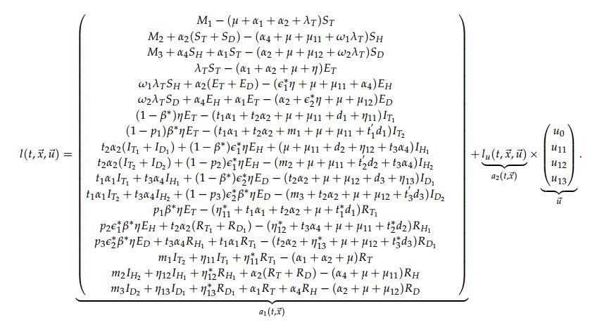
Proof. Let \[F(S, 0)= \begin{pmatrix} M_{1}-(\mu +\alpha_{1}+\alpha_{2}) S_{T} \\ M_{2}-(\mu +\mu_{11}+\alpha_{4}) S_{H} \\ M_{3}-(\mu+\mu_{12} +\alpha_{1}) S_{D} \\ 0\\ 0\\ 0 \end{pmatrix}.\] As \(F(S, 0)\) is a linear equation, we have that \(S^{*}_{0}\) is globally stable, hence \(H_{1}\) is satisfied. Then, \begin{align*} \mathbf{A}&={\tiny\left(\begin{array}{cccccccccccc} -k_{11} & 0 &0& \alpha^{*}& \alpha^{*} & \alpha^{*}\epsilon_{1} & \alpha^{*}\epsilon_{1}& \alpha^{*}\epsilon_{2} & \alpha^{*}\epsilon_{2} &\alpha^{*}& \alpha^{*}\epsilon_{1} & \alpha^{*}\epsilon_{2}\\ \alpha_{2} &-k_{21} &\alpha_{2}& \omega_{1}\alpha^{*}& \omega_{1}\alpha^{*} & \omega_{1}\alpha^{*}\epsilon_{1} & \omega_{1}\alpha^{*}\epsilon_{1}& \omega_{1}\alpha^{*}\epsilon_{2} & \omega_{1}\alpha^{*}\epsilon_{2}&\omega_{1}\alpha^{*}& \omega_{1}\alpha^{*}\epsilon_{1} & \omega_{1}\alpha^{*}\epsilon_{2} \\ \alpha_{1} &\alpha_{4} &-k_{31}& \omega_{2}\alpha^{*}& \omega_{2}\alpha^{*} & \omega_{2}\alpha^{*}\epsilon_{1} & \omega_{2}\alpha^{*}\epsilon_{1}& \omega_{2}\alpha^{*}\epsilon_{2} & \omega_{2}\alpha^{*}\epsilon_{2} &\omega_{2}\alpha^{*}& \omega_{2}\alpha^{*}\epsilon_{1} & \omega_{2}\alpha^{*}\epsilon_{2}\\ (1-\beta^{*})\eta & 0 & 0& -k_{12} & 0&0 &0 &0& 0&0 &0 &0 \\ (1-p_{1})\beta^{*}\eta & 0 & 0& l_{1} & -k_{13}&0 &0 &0& 0&0 &0 &0 \\ 0& (1-\beta^{*})\epsilon^{*}_{1}\eta & 0&\alpha_{2} & 0&-k_{22} &\alpha_{2} &0& 0&0 &0 &0 \\ 0& (1-P_{2})\beta^{*}\epsilon^{*}_{1}\eta & 0& 0&\alpha_{2} &l_{2} &-k_{23} &0& \alpha_{2}&0 &0 &0 \\ 0& 0&(1-\beta^{*})\epsilon^{*}_{2}\eta &\alpha_{1} & 0&\alpha_{4} &0 &-k_{32}& 0&0 &0 &0 \\ 0& 0&(1-p_{3})\beta^{*}\epsilon^{*}_{2}\eta &0 & \alpha_{1}&0 &\alpha_{4} &l_{3}& -k_{33}&0 &0 &0 \\ p_{1}\beta^{*}\eta & 0 & 0 &0 & \eta_{14}& 0& 0&0 & 0&-k_{14} &0 &0\\ 0& p_{2}\epsilon^{*}_{1}\beta^{*}\eta & 0 &0 & 0& 0& \eta_{15}&0 & 0&\alpha_{2} &-k_{24} &\alpha_{2}\\ 0& 0 & p_{3}\epsilon^{*}_{2}\beta^{*}\eta &0 & 0& 0& 0&0 & \eta_{16}&\alpha_{1} &\alpha_{4} &-k_{34}\\ \end{array}\right)},\\ \mathbf{I}&=\left(\begin{array}{cccccccccccc} E_{T}, &E_{H}, & E_{D}, & I_{T_{1}}, & I_{T_{2}}, & I_{H_{1}}, & I_{H_{2}}, & I_{D_{1}}, & I_{D_{2}}, & R_{T_{1}}, & R_{H_{1}}, & R_{D_{1}} \\ \end{array}\right),\\ G^{*}(S,I)&=AI^{T}-G(S,I),\\ G^{*}(S,I)&={\small\begin{pmatrix} G^{*}_{1}(S,I) \\ G^{*}_{2}(S,I)\\ G^{*}_{3}(S,I)\\ G^{*}_{4}(S,I)\\ G^{*}_{5}(S,I) \\ G^{*}_{6}(S,I)\\ G^{*}_{7}(S,I)\\ G^{*}_{8}(S,I)\\ G^{*}_{9}(S,I) \\ G^{*}_{10}(S,I)\\ G^{*}_{11}(S,I)\\ G^{*}_{12}(S,I) \end{pmatrix}=\begin{pmatrix} \alpha^{*}(I_{T_{1}}+I_{T_{2}}+R_{T_{1}}+\epsilon_{1}({I_{H_{1}}+I_{H_{2}}+R_{H_{1}}})+\epsilon_{2}(I_{D_{1}}+I_{D_{2}}+R_{D_{1}}))\bigg( 1- \dfrac{S_{T}+\beta^{‘}_{1}R_{T}}{N}\bigg) \\ \omega_{1}\alpha^{*}(I_{T_{1}}+I_{T_{2}}+R_{T_{1}}+\epsilon_{1}({I_{H_{1}}+I_{H_{2}}+R_{H_{1}}})+\epsilon_{2}(I_{D_{1}}+I_{D_{2}}+R_{D_{1}}))\bigg( 1- \dfrac{S_{H}+\beta^{‘}_{1}R_{H}}{N}\bigg) \\ \omega_{2}\alpha^{*}(I_{T_{1}}+I_{T_{2}}+R_{T_{1}}+\epsilon_{1}({I_{H_{1}}+I_{H_{2}}+R_{H_{1}}})+\epsilon_{2}(I_{D_{1}}+I_{D_{2}}+R_{D_{1}}))\bigg( 1- \dfrac{S_{D}+\beta^{‘}_{1}R_{D}}{N}\bigg) \\ 0\\ 0\\ 0\\ 0\\ 0\\ 0\\ 0\\ 0\\ 0 \end{pmatrix}}. \end{align*} Since \(S_{T}+\beta^{‘}_{1}R_{T}\), \(S_{H}+\beta^{‘}_{1}R_{H}\) and \(S_{D}+\beta^{‘}_{1}R_{D}\) are always less than or equal to \(N_{T},\) \(\dfrac{S_{T}+\beta^{‘}_{1}R_{T}}{N}\leq 1\), \(\dfrac{S_{H}+\beta^{‘}_{1}R_{H}}{N}\leq 1\) and \(\dfrac{S_{D}+\beta^{‘}_{1}R_{D}}{N}\leq 1.\) Thus \(G^{*}(S,I) \geq 0\) for all \((S,I) \in D.\) The \(E_{0}^{G}\) is a globally asymptotically stable.
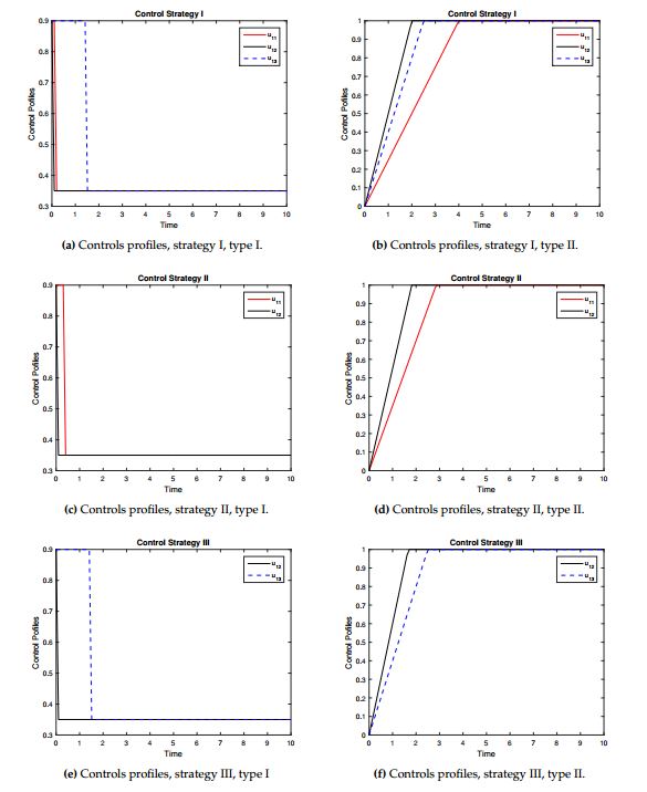
In particular, \(u_{11}(t)\) is the control in the entrance to compartment \(I_{T_{2}}\), \(R_{T_{1}}\), \(u_{12}(t)\) is the control in the entrance to compartment \(I_{H_{2}}\), \(R_{H_{1}}\) and \(u_{13}(t)\) is the control in the entrance to compartment \(I_{D_{2}}\), \(R_{D_{1}}\). The \(u_{0}(t)\) controls entry into the \(E_{T}\), \(E_{H}\) and \(E_{D}\) compartments by reinfection or reactivation. Eqs (7) shows the incorporation of the controls in the compartments of model (1) and the other equations remain the same as the uncontrolled model (1). The \((1-u_{0})\), \((1-u_{11})\), \((1-u_{12})\) and \((1-u_{13})\) representing effort that prevents failure of the treatment. The Figure 1 shows the control dynamics.

The coefficients \(B_{j}, j = 0,1,…,6\) represent the constant weight associated with the relative costs of implementing the respective control strategies on a finite time horizon \([t_{0}, t_{f}]\) (were initial time \(t_{0}=0\), final time \(t_{f}=10\) year period) and consists in the cost induced by the efforts of the three different types of control. The \(B_{1}\), \(B_{2}\) and \(B_{3}\) are associated with the implementation of control on the MDR-TB and \(B_{4}\), \(B_{5}\) and \(B_{6}\) to the XDR-TB. Given the characteristics of resistance to tuberculosis and its treatment, which in some cases may include hospitalization, high drug costs, the use of other drugs to stimulate the immune system, among others, let’s assume that \(B_{1}< B_{4}\), \(B_{2}< B_{5}\) and \(B_{3}< B_{6}\) and these constants cannot be neither zeros nor very large (realistic values). Given the characteristics of resistance to tuberculosis and its treatment, which in some cases may include hospitalization, high drug costs, the use of other drugs to stimulate the immune system, among others, let's assume that \(B_{1}< B_{4}\), \(B_{2}< B_{5}\) and \(B_{3}< B_{6}\) and these constants cannot be neither zeros nor very large (realistic values).
The cost involved in the control about the compartments \(I_{T_{2}}\), \(I_{H_{2}}\) and \(I_{D_{2}}\) is taken as \(\int^{t_{f}}_{t_{0}}\frac{B_{1}u^{2}_{11}}{2}\), \(\int^{t_{f}}_{t_{0}}\frac{B_{2}u^{2}_{12}}{2}\), \(\int^{t_{f}}_{t_{0}}\frac{B_{3}u^{2}_{13}}{2}\), for \(R_{T_{1}}\), \(R_{H_{1}}\), \(R_{D_{1}}\) are \(\int^{t_{f}}_{t_{0}}\frac{B_{4}u^{2}_{11}}{2}\), \(\int^{t_{f}}_{t_{0}}\frac{B_{5}u^{2}_{12}}{2}\), \(\int^{t_{f}}_{t_{0}}\frac{B_{6}u^{2}_{13}}{2}\), for \(E_{T}\), \(E_{H}\) and \(E_{D}\) are \(\int^{t_{f}}_{t_{0}}\frac{B_{0}u^{2}_{0}}{2}\). We seek to find the optimal controls \(u^{*}_{0}\), \(u^{*}_{11}\), \(u^{*}_{0}\), \(u^{*}_{12}\) and \(u^{*}_{13}\) that satisfy
We denote the vector of states \(\vec{x}=[S_{T}, S_{H}, S_{D}, E_{T}, E_{H}, E_{D}, I_{T_{1}}, I_{T_{2}}, I_{H_{1}},I_{H_{2}}, I_{D_{1}}, I_{D_{2}}, R_{T_{1}}, R_{H_{1}}, R_{D_{1}}, R_{T}, R_{H}, R_{D}]^{T}\) and the controls vector \(\vec{u}=[u_{0},u_{11}, u_{12}, u_{13}]^{T}\).
Theorem 4. There exists an optimal control \(u^{*}=(u^{*}_{0}, u^{*}_{11}, u^{*}_{12}, u^{*}_{13})\) to problem \[\min J(u_{0}, u_{11}, u_{12}, u_{13}) \quad \text{subject to model (1) with controls}\] where \(u^{*}\in U_{ad}.\)
Proof. We use the requirements of Theorem 4.1 and Corollary 4.2 in [28] to prove the Theorem 4. Let \(l(t, \vec{x}, \vec{u})\) as the right-hand of (1) with controls. We will show that the following requirements are satisfied:
\(\vert l(t,0,0)\vert \leq C\), \(\vert l_{x}(t, \vec{x}, \vec{u})\vert \leq C(1+\vert \vec{u}\vert)\), \(\vert l_{u}(t, \vec{x}, \vec{u}) \vert \leq C\).
By the construction of the model and the condition I., system (1) with controls has a unique solution for constant controls, this implies that condition II. is satisfied.
We can write the system (1) with controls as
This means that condition III. holds. By construction the sets \(U\) is closed, convex and compact and condition IV. is satisfied.
Now, we are going to prove the convexity of the integrand in the objective functional
\begin{align*} \label{h1} f(t, \vec{x}, \vec{u})=&E_{T}(t)+E_{H}(t)+E_{D}(t)+I_{T_{2}}(t)+I_{H_{2}}(t)+I_{D_{2}}(t)+I_{T_{3}}(t)+I_{H_{3}}(t)+I_{D_{3}}(t)+ \dfrac{B_{0}u^{2}_{0}(t)}{2}\\ \nonumber &+\dfrac{(B_{1}+B_{4})u_{11}^{2}(t)}{2}+\dfrac{(B_{2}+B_{5})u_{12}^{2}(t)}{2}+\dfrac{(B_{3}+B_{6})u_{13}^{2}(t)}{2}, \end{align*} this implies proving that \[(1-q)f(t, \vec{x}, \vec{u})+qf(t, \vec{x}, \vec{v}) \geq f(t, \vec{x}, (1-q)\vec{u}+q\vec{v}),\] where \(\vec{u}\), \(\vec{v}\) are two control vectors with \(q\in [0,1]\). It follows that \begin{align*} &(1-q)f(t, \vec{x}, \vec{u})+qf(t, \vec{x}, \vec{v})= (1-q)\bigg(E_{T}+E_{H}+E_{D}+I_{T_{2}}+I_{H_{2}}+I_{D_{2}}+I_{T_{3}}+I_{H_{3}}+I_{D_{3}}+\dfrac{B_{0}u^{2}_{0}}{2}+\dfrac{(B_{1}+B_{4})u_{11}^{2}}{2}\\ &+\dfrac{(B_{2}+B_{5})u_{12}^{2}}{2}+ \dfrac{(B_{3}+B_{6})u_{13}^{2}}{2}\bigg) +q\bigg(E_{T}+E_{H}+E_{D}+I_{T_{2}}+I_{H_{2}}+I_{D_{2}}+I_{T_{3}}+I_{H_{3}}+I_{D_{3}} +\dfrac{B_{0}v^{2}_{0}}{2}+\dfrac{(B_{1}+B_{4})v_{11}^{2}}{2}\\ &+\dfrac{(B_{2}+B_{5})v_{12}^{2}}{2}+ \dfrac{(B_{3}+B_{6})v_{13}^{2}}{2}\bigg)\\ &= E_{T}+E_{H}+E_{D}+I_{T_{2}}+I_{H_{2}}+I_{D_{2}}+I_{T_{3}}+I_{H_{3}}+I_{D_{3}}+\bigg( \dfrac{B_{0}(qv^{2}_{0}+(1-q)u^{2}_{0})}{2}+ \dfrac{(B_{1}+B_{4})(qv_{11}^{2}+(1-q)u_{11}^{2})}{2}\\ &+ \dfrac{(B_{2}+B_{5})(qv_{12}^{2}+(1-q)u_{12}^{2})}{2}+\dfrac{(B_{3}+B_{6})(qv_{13}^{2}+(1-q)u_{13}^{2})}{2}\bigg) \end{align*} and \begin{align*} & f(t, \vec{x}, (1-q)\vec{u}+q\vec{v})= (E_{T}+E_{H}+E_{D}+I_{T_{2}}+I_{H_{2}}+I_{D_{2}}+I_{T_{3}}+I_{H_{3}}+I_{D_{3}}+\dfrac{B_{0}}{2}\bigg[(1-q)u_{0}+qv_{0}\bigg]^{2}\\ &+\dfrac{(B_{1}+B_{4})}{2}\bigg[(1-q)u_{11}+qv_{11}\bigg]^{2}+\dfrac{(B_{2}+B_{5})}{2}\bigg[(1-q)u_{12}+qv_{12}\bigg]^{2}+\dfrac{(B_{3}+B_{6})}{2}\bigg[(1-q)u_{13}+qv_{13}\bigg]^{2}. \end{align*} Then, we have \begin{align*} &(1-q)f(t, \vec{x}, \vec{u})+qf(t, \vec{x}, \vec{v})-f(t, \vec{x}, (1-q)\vec{u}+q\vec{v})\\ &= \dfrac{B_{0}}{2}\bigg((1-q)u^{2}_{0}+ q v^{2}_{0}-((1-q)u_{0}+qv_{0})^{2}\bigg)+ \dfrac{(B_{1}+B_{4})}{2}\bigg((1-q)u^{2}_{11}+ q v^{2}_{11}-((1-q)u_{11}+qv_{11})^{2}\bigg)\\ &+\dfrac{(B_{2}+B_{5})}{2}\bigg((1-q)u^{2}_{12}+ q v^{2}_{12}-((1-q)u_{12}+qv_{12})^{2}\bigg)+\dfrac{(B_{3}+B_{6})}{2}\bigg((1-q)u^{2}_{13}+ q v^{2}_{13}-((1-q)u_{13}+qv_{13})^{2}\bigg)\\ &=\dfrac{B_{0}}{2}\bigg[\sqrt{q(1-q)}u_{0}-\sqrt{q(1-q)}v_{0}\bigg]^{2}+ \dfrac{(B_{1}+B_{4})}{2}\bigg[\sqrt{q(1-q)}u_{11}-\sqrt{q(1-q)}v_{11}\bigg]^{2}\\ &+\dfrac{(B_{2}+B_{5})}{2}\bigg[\sqrt{q(1-q)}u_{12}-\sqrt{q(1-q)}v_{12}\bigg]^{2}+ \dfrac{(B_{3}+B_{6})}{2}\bigg[\sqrt{q(1-q)}u_{13}-\sqrt{q(1-q)}v_{13}\bigg]^{2}\geq 0. \end{align*} With this, we prove the requirement V. and the proof of the theorem is complete. The Pontryagin’s Maximum Principle, provides the necessary conditions an optimal control must satisfy. Firstly, the Hamiltonian for the control problem is defined byTheorem 5. Given an optimal controls \(u^{*}_{0}, u^{*}_{11}\), \(u^{*}_{12}\), \(u^{*}_{13}\) and associated solutions \(S^{*}_{T}\), \(S^{*}_{H}\), \(S^{*}_{D}\), \(E^{*}_{T}\), \(E^{*}_{H}\), \(E^{*}_{D}\), \(I^{*}_{T_{1}}\), \(I^{*}_{T_{2}}\), \(I^{*}_{H_{1}}\), \(I^{*}_{H_{2}}\), \(I^{*}_{D_{1}}\), \(I^{*}_{D_{2}}\), \(R^{*}_{T}\), \(R^{*}_{H}\) and \(R^{*}_{D}\), that minimizes \(J(u_{0}, u_{11}, u_{12}, u_{13})\) over the domain \(U_{ad}\), there exist adjoint function, \(\lambda_{i}(t)\), \(i=1,..,18\) that satisfy: \[ \dfrac{d\lambda_{i}}{dt}=-\dfrac{\partial H}{\partial x_{i}}\] where \(x_{i}=\) \(S_{T}\), \(S_{H}\), \(S_{D}\), \(E_{T}\), \(E_{H}\), \(E_{D}\), \(I_{T_{1}}\), \(I_{T_{2}}\), \(I_{H_{1}}\), \(I_{H_{2}}\), \(I_{D_{1}}\), \(I_{D_{2}}\), \(R_{T}\), \(R_{H}\), \(R_{D}\). In association with the transversality conditions \(\lambda_{l}(t_{f})=0\) for \(l=1,2,…, 18.\) Moreover, the following characterization holds
Proof. Using Pontryagin’s Maximum Principle [29], the adjoint equations are obtained: \begin{align} \dfrac{d \lambda_{1}}{dt}= -\dfrac{\partial H}{\partial S_{T}}&= \alpha_{1}(\lambda_{1}-\lambda_{3})+\alpha_{2}(\lambda_{1}-\lambda_{2})+\lambda_{T}(\lambda_{1}- \lambda_{4})+\mu \lambda_{1}, \nonumber \\ \dfrac{d \lambda_{2}}{dt}= -\dfrac{\partial H}{\partial S_{H}}&= \alpha_{4}(\lambda_{2}-\lambda_{3})+\omega_{1}\lambda_{T}(\lambda_{2}- \lambda_{5})+(\mu+\mu_{11}) \lambda_{2}, \nonumber \\ \dfrac{d \lambda_{3}}{dt}= -\dfrac{\partial H}{\partial S_{D}}&= \alpha_{2}(\lambda_{3}-\lambda_{2})+\omega_{2}\lambda_{T}(\lambda_{3}- \lambda_{6})+(\mu+\mu_{12}) \lambda_{3}, \nonumber \\ \dfrac{d \lambda_{4}}{dt}= -\dfrac{\partial H}{\partial E_{T}}&=-1+\alpha_{1}(\lambda_{4}-\lambda_{6})+\alpha_{2}(\lambda_{4}-\lambda_{5})+\eta((\lambda_{4}-\lambda_{7})+\beta^{*}((\lambda_{7}-\lambda_{8})+p_{1}(\lambda_{8}-\lambda_{13})))+\mu \lambda_{4}, \nonumber \\ \dfrac{d \lambda_{5}}{dt}= -\dfrac{\partial H}{\partial E_{H}}&=-1+\alpha_{4}(\lambda_{5}-\lambda_{6})+\eta\epsilon^{*}_{1}((\lambda_{5}-\lambda_{9})+\beta^{*}((\lambda_{9}-\lambda_{10})+p_{2}(\lambda_{10}-\lambda_{14})))+(\mu+\mu_{11}) \lambda_{5}, \nonumber\\ \dfrac{d \lambda_{6}}{dt}= -\dfrac{\partial H}{\partial E_{D}}&= -1+\alpha_{2}(\lambda_{6}-\lambda_{5})+\eta\epsilon^{*}_{2}((\lambda_{6}-\lambda_{11})+\beta^{*}((\lambda_{11}-\lambda_{12})+p_{3}(\lambda_{12}-\lambda_{15})))+(\mu+\mu_{12}) \lambda_{6}, \nonumber \\ \dfrac{d \lambda_{7}}{dt}=-\dfrac{\partial H}{\partial I_{T_{1}}}&=-1+ t_{1}\alpha_{1}(\lambda_{7}-\lambda_{11})+t_{2}\alpha_{2}(\lambda_{7}-\lambda_{9})+\eta_{11}(\lambda_{7}-\lambda_{16})+(1-u_{11})l_{1}(\lambda_{7}-\lambda_{8}) \nonumber \\ \dfrac{d \lambda_{8}}{dt}=-\dfrac{\partial H}{\partial I_{T_{2}}}&=-1+(1-u_{11})\eta_{14}(\lambda_{8}-\lambda_{13})+t_{1}\alpha_{1}(\lambda_{8}-\lambda_{12})+t_{2}\alpha_{2}(\lambda_{8}-\lambda_{10})+m_{1}(\lambda_{8}-\lambda_{16}) & \nonumber \\ & + \dfrac{\alpha^{*}}{N}\big((\lambda_{1}-\lambda_{4})S_{T}+\omega_{1}S_{H}(\lambda_{2}-\lambda_{5})+\omega_{2}S_{D}(\lambda_{3}-\lambda_{6})+(1-u_{0})\beta^{‘}_{1}(R_{T}(\lambda_{16}-\lambda_{4}) & \nonumber \\ &+ \omega_{1}R_{H}(\lambda_{17}-\lambda_{5})+\omega_{2}R_{D}(\lambda_{18}-\lambda_{6}))\big)+(\mu+t^{‘}_{1}d_{1})\lambda_{8}, & \nonumber \\ \dfrac{d \lambda_{9}}{dt}=-\dfrac{\partial H}{\partial I_{H_{1}}}&=-1+ (1-u_{12})l_{2}(\lambda_{9}-\lambda_{10})+\eta_{12}(\lambda_{9}-\lambda_{17})+t_{3}\alpha_{4}(\lambda_{9}-\lambda_{11})& \nonumber \\ &+\dfrac{\alpha^{*}}{N}\epsilon_{1}\big((\lambda_{1}-\lambda_{4})S_{T}+\omega_{1}S_{H}(\lambda_{2}-\lambda_{5})+\omega_{2}S_{D}(\lambda_{3}-\lambda_{6})+(1-u_{0})\beta^{‘}_{1}(R_{T}(\lambda_{16}-\lambda_{4}) & \nonumber \\ &+\omega_{1}R_{H}(\lambda_{17}-\lambda_{5})+\omega_{2}R_{D}(\lambda_{18}-\lambda_{6}))\big)+(\mu+\mu_{11}+d_{2})\lambda_{9},& \nonumber \\ \dfrac{d \lambda_{10}}{dt}=-\dfrac{\partial H}{\partial I_{H_{2}}}&=-1+\dfrac{\alpha^{*}}{N}\epsilon_{1}\big((\lambda_{1}-\lambda_{4})S_{T}+\omega_{1}S_{H}(\lambda_{2}-\lambda_{5})+\omega_{2}S_{D}(\lambda_{3}-\lambda_{6})+(1-u_{0})\beta^{‘}_{1}(R_{T}(\lambda_{16}-\lambda_{4})& \nonumber \\& +\omega_{1}R_{H}(\lambda_{17}-\lambda_{5})+\omega_{2}R_{D}(\lambda_{18}-\lambda_{6}))\big)+t_{3}\alpha_{4}(\lambda_{10}-\lambda_{12})+m_{2}(\lambda_{10}-\lambda_{17})+(1-u_{11})\eta_{15}(\lambda_{10}& \nonumber \\ &- \lambda_{14})+ (\mu+\mu_{11}+t^{‘}_{2}d_{2})\lambda_{10}, & \nonumber \\ \dfrac{d \lambda_{11}}{dt}=-\dfrac{\partial H}{\partial I_{D_{1}}}&=-1+\dfrac{\alpha^{*}}{N}\epsilon_{2}\big((\lambda_{1}-\lambda_{4})S_{T}+\omega_{1}S_{H}(\lambda_{2}-\lambda_{5})+\omega_{2}S_{D}(\lambda_{3}-\lambda_{6})+(1-u_{0})\beta^{‘}_{1}(R_{T}(\lambda_{16}-\lambda_{4})& \nonumber \\ &+\omega_{1}R_{H}(\lambda_{17}-\lambda_{5})+\omega_{2}R_{D}(\lambda_{18}-\lambda_{6}))\big)+ (1-u_{13})l_{3}(\lambda_{11}-\lambda_{12})+\eta_{13}(\lambda_{11}-\lambda_{18})& \nonumber \\ &+t_{2}\alpha_{2}(\lambda_{11}-\lambda_{9})+(\mu+\mu_{12}+d_{3})\lambda_{11}, & \nonumber \end{align} \begin{align}\label{tranve1} \dfrac{d \lambda_{12}}{dt}=-\dfrac{\partial H}{\partial I_{D_{2}}}&=-1+ \dfrac{\alpha^{*}}{N}\epsilon_{2}\big((\lambda_{1}-\lambda_{4})S_{T}+\omega_{1}S_{H}(\lambda_{2}-\lambda_{5})+\omega_{2}S_{D}(\lambda_{3}-\lambda_{6})+(1-u_{0})\beta^{‘}_{1}(R_{T}(\lambda_{16}-\lambda_{4})& \nonumber \\ &+\omega_{1}R_{H}(\lambda_{17}-\lambda_{5})+\omega_{2}R_{D}(\lambda_{18}-\lambda_{6}))\big)+t_{2}\alpha_{2}(\lambda_{12}-\lambda_{10})+m_{3}(\lambda_{12}-\lambda_{18}) & \nonumber \\ &+(1-u_{13})\eta_{16}(\lambda_{12}-\lambda_{15})+(\mu+\mu_{12}+t^{‘}_{3}d_{3})\lambda_{12}, & \nonumber \\ \dfrac{d \lambda_{13}}{dt}=-\dfrac{\partial H}{\partial R_{T_{1}}}&=-1+ \dfrac{\alpha^{*}}{N}\big((\lambda_{1}-\lambda_{4})S_{T}+\omega_{1}S_{H}(\lambda_{2}-\lambda_{5})+\omega_{2}S_{D}(\lambda_{3}-\lambda_{6})+(1-u_{0})\beta^{‘}_{1}(R_{T}(\lambda_{16}-\lambda_{4}) & \nonumber \\ &+\omega_{1}R_{H}(\lambda_{17}-\lambda_{5})+\omega_{2}R_{D}(\lambda_{18}-\lambda_{6}))\big)+\eta^{*}_{11}(\lambda_{13}-\lambda_{16})+t_{1}\alpha_{1}(\lambda_{13}-\lambda_{15})& \nonumber \\ &+t_{2}\alpha_{2}(\lambda_{13}-\lambda_{14})+(\mu+t^{*}_{1}d_{1})\lambda_{13},& \nonumber \\ \dfrac{d \lambda_{14}}{dt}=-\dfrac{\partial H}{\partial R_{H_{1}}}&=-1+ \dfrac{\alpha^{*}}{N}\epsilon_{1}\big((\lambda_{1}-\lambda_{4})S_{T}+\omega_{1}S_{H}(\lambda_{2}-\lambda_{5})+\omega_{2}S_{D}(\lambda_{3}-\lambda_{6})+(1-u_{0})\beta^{‘}_{1}(R_{T}(\lambda_{16}-\lambda_{4})& \nonumber \\ &+\omega_{1}R_{H}(\lambda_{17}-\lambda_{5})+\omega_{2}R_{D}(\lambda_{18}-\lambda_{6}))\big)+ \eta^{*}_{12}(\lambda_{14}-\lambda_{17})+t_{3}\alpha_{4}(\lambda_{14}-\lambda_{15})& \nonumber \\ &+(\mu+\mu_{11}+t^{*}_{2}d_{2})\lambda_{14},& \nonumber \\ \dfrac{d \lambda_{15}}{dt}=-\dfrac{\partial H}{\partial R_{D_{1}}}&=-1+ \dfrac{\alpha^{*}}{N}\epsilon_{2}\big((\lambda_{1}-\lambda_{4})S_{T}+\omega_{1}S_{H}(\lambda_{2}-\lambda_{5})+\omega_{2}S_{D}(\lambda_{3}-\lambda_{6})+(1-u_{0})\beta^{‘}_{1}(R_{T}(\lambda_{16}-\lambda_{4})& \nonumber \\ &+\omega_{1}R_{H}(\lambda_{17}-\lambda_{5})+\omega_{2}R_{D}(\lambda_{18}-\lambda_{6}))\big)+\eta^{*}_{13}(\lambda_{15}-\lambda_{18})+t_{2}\alpha_{2}(\lambda_{15}-\lambda_{14})& \nonumber \\ &+(\mu+\mu_{12}+t^{*}_{3}d_{3})\lambda_{15},& \nonumber \\ \dfrac{d \lambda_{16}}{dt}=-\dfrac{\partial H}{\partial R_{T}}&=(1-u_{0})\beta^{‘}_{1}\lambda_{T}(\lambda_{16}-\lambda_{4})+\alpha_{1}(\lambda_{16}-\lambda_{18})+\alpha_{2}(\lambda_{16}-\lambda_{17})+\mu \lambda_{16}, & \nonumber \\ \dfrac{d \lambda_{17}}{dt}=-\dfrac{\partial H}{\partial R_{H}}&=(1-u_{0})\beta^{‘}_{1}\lambda_{T}\omega_{1}(\lambda_{17}-\lambda_{5})+\alpha_{4}(\lambda_{17}-\lambda_{18})+(\mu+\mu_{11}) \lambda_{17},& \nonumber \\ \dfrac{d \lambda_{18}}{dt}=-\dfrac{\partial H}{\partial R_{D}}&=(1-u_{0})\beta^{‘}_{1}\lambda_{T}\omega_{2}(\lambda_{18}-\lambda_{6})+\alpha_{2}(\lambda_{18}-\lambda_{17})+(\mu+\mu_{12}) \lambda_{18}. & \end{align} Optimality is when the equations \(\dfrac{\partial H}{\partial u_{j}}=0\) at \(u^{*}_{0}\), \(u^{*}_{1i}\) for \(i=1, 2, 3\). Then, \[\dfrac{\partial H}{\partial u_{0}}=B_{0}u_{0}+\beta^{‘}_{1}\lambda_{T}\big((\lambda_{16}-\lambda_{4})R_{T}+\omega_{1}(\lambda_{17}-\lambda_{5})R_{H}+\omega_{2}(\lambda_{18}-\lambda_{6})R_{D}\big)=0\,,\] which implies that \[u^{*}_{0}=\dfrac{\beta^{‘}_{1}\lambda_{T}\big((\lambda_{4}-\lambda_{16})R_{T}+\omega_{1}(\lambda_{5}-\lambda_{17})R_{H}+\omega_{1}(\lambda_{6}-\lambda_{18})R_{D}\big)}{B_{0}}\,,\] on the set \(\lbrace t: 0< u^{*}_{0}(t)< 1 \rbrace\). \[\dfrac{\partial H}{\partial u_{11}}=(B_{1}+B_{4})u_{11}+l_{1}I_{T_{1}}(\lambda_{7}-\lambda_{8})+\eta_{14}I_{T_{2}}(\lambda_{8}-\lambda_{13})R_{D}=0\,,\] which implies that \[u^{*}_{11}=\dfrac{l_{1}I_{T_{1}}(\lambda_{8}-\lambda_{7})+\eta_{14}I_{T_{2}}(\lambda_{13}-\lambda_{8})}{B_{1}+B_{4}}\,,\] on the set \(\lbrace t: 0< u^{*}_{11}(t)< 1 \rbrace\).
Analogously, for the optimal control \(u^{*}_{12}\), we have
\[\dfrac{\partial H}{\partial u_{12}}=(B_{2}+B_{5})u_{12}+l_{2}I_{H_{1}}(\lambda_{9}-\lambda_{10})+\eta_{15}I_{H_{2}}(\lambda_{10}-\lambda_{14})R_{H}=0.\] Therefore, \[u^{*}_{12}= \dfrac{l_{2}I_{H_{1}}(\lambda_{10}-\lambda_{9})+\eta_{15}I_{H_{2}}(\lambda_{14}-\lambda_{10})}{B_{2}+B_{5}}\,,\] on the set \(\lbrace t: 0< u^{*}_{12}(t)< 1 \rbrace\). For the control \(u^{*}_{13}\), we obtained \[\dfrac{\partial H}{\partial u_{13}}=(B_{3}+B_{6})u_{13}+l_{3}I_{D_{1}}(\lambda_{11}-\lambda_{12})+\eta_{16}I_{D_{2}}(\lambda_{12}-\lambda_{15})=0,\] and this implies that \[u^{*}_{13}= \dfrac{l_{3}I_{D_{1}}(\lambda_{12}-\lambda_{11})+\eta_{16}I_{D_{2}}(\lambda_{15}-\lambda_{12})}{B_{3}+B_{6}}\,,\] on the control set \(\lbrace t: 0< u^{*}_{13}(t)< 1\rbrace \).Note that the optimality conditions only hold on the interior of the control set.
For the numerical simulations, we use a set of parameters extracted from [31,32,33,34,35,36,37,38,39,40,41] with purposes illustrative and to support the analytical results, see Table 2.
The initial conditions for the TB-Only and TB-Diabetes sub-populations are taken from [31], and the values for th1e sub-population of HIV/AIDS are assumed and do not represent a specific demographic area, but fall within the range of actual achievable data, see Table 2. The values of the parameters and initial conditions that are assumed are discussed and validated with the specialists. We assume that \(B_{0}=200\), \(B_{1}=50\), \(B_{2}=150\), \(B_{3}=75\), \(B_{4}=100\), \(B_{5}=250\) and \(B_{3}=150\).
We assume that always apply control in the HIV/AIDS sub-population because tuberculosis is classified as an opportunistic disease and HIV/AIDS cases are monitored by the use of antiretroviral therapy. Also, reinfection or reactivation of TB is always controlled in all strategies because of its impact on treatment resistance. Then, our control strategies are defined as the combination of efforts and are defined as:
Strategy I. We activate all controls (\(u_{0}(t), u_{11}(t), u_{12}(t)>0, u_{13}(t)>0\)).
Strategy II. Combination of \(u_{0}(t)\), \(u_{11}(t)\), \(u_{12}(t)\) while setting \(u_{13}(t)=0\) (\(u_{0}(t), u_{11}(t)>0, u_{12}(t)>0\) and \(u_{13}(t)=0\)).
Strategy III. Combination of \(u_{0}(t)\), \(u_{12}(t)\), \(u_{13}(t)\) while setting \(u_{11}(t)=0\) (\(u_{0}(t),u_{12}(t),u_{13}(t)>0\) and \(u_{11}(t)=0\)).
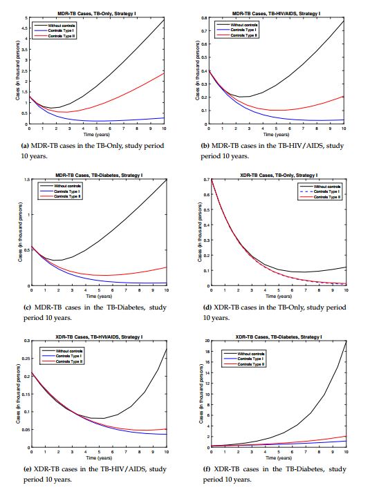
We are going to study how we start the control process, with high efficient control (type I) and with minimum value (type II). Figure 2 shows the profiles of the resistance controls (\(u_{11}(t), u_{12}(t), u_{13}(t)\)) over time for the different strategies and control types.Strategy I. In this strategy all controls are active (\(u_{0}(t)>0\), \(u_{11}(t)>0\), \(u_{12}(t)>0\) and \(u_{13}(t)>0\)). In other words, reinfection or reactivation and resistance are controlled. We show the behavior of the controls over time, see Figure 2a for control type I and see Figure 2b for control type II. It is observed that when this control strategy is implemented, there is a significant decrease in the number of TB resistant compared with the model without control, see Figure 3. In the case of MDR-TB in the different sub-populations before the study year, a decrease in the number of reported cases was observed, see Figures 3a-3c. In the case of XR-TB, the reduction in the number of cases will occur over a longer period of time, but this reduction is significant, mainly in XDR-TB diabetics, which has a strong incidence in the dynamics, see Figure 3d-3f. In the case of MDR-TB and XDR-TB in the TB-HIV/AIDS sub-population, the control manages to avoid the growth of the number of cases because in the dynamics these compartments tend to decrease initially and then grow. This strategy takes advantage of the decrease in the number of cases by preventing future growth. The type I control showed better results so it is recommended to start with higher efficacy and this evolves showing better results.
Strategy II. Here we activate the controls \(u_{0}(t)>0\), \(u_{11}(t)>0\) and \(u_{12}(t)>0\) and \(u_{13}(t)=0\), this means that we control resistance in the TB-HIV/AIDS and TB-Only sub-populations and reinfection or reactivation TB in the full model. The behavior of the controls is shown in Figure 2c-2d.
| Variables | Value | Variables | Value | Variables | Value |
|---|---|---|---|---|---|
| \(S_{T}(0) \) | 8741400 | \(S_{H}(0) \) | 111000 | \(S_{D}(0) \) | 200000 |
| \(E_{T}(0) \) | 565600 | \(E_{H}(0) \) | 5000 | \(E_{D}(0) \) | 8500 |
| \(I_{T_{1}}(0) \) | 20000 | \(I_{H_{1}}(0) \) | 1400 | \(I_{D_{1}}(0) \) | 1800 |
| \(I_{T_{2}}(0) \) | 1300 | \(I_{H_{2}}(0) \) | 400 | \(I_{D_{2}}(0) \) | 550 |
| \(R_{T_{1}}(0) \) | 700 | \(R_{H_{1}}(0) \) | 210 | \(R_{D_{1}}(0) \) | 250 |
| \(R_{T}(0) \) | 8800 | \(R_{H}(0) \) | 500 | \(R_{D}(0) \) | 300 |
| Parameters | Value | Reference | Parameters | Value | Reference |
| \(M_{1}, \) \(M_{2}, \) \(M_{3} \) | \(667685, 10000, 50000 \) | [31], Assumed, Assumed | \(\alpha^{*} \) | \( 9.5 \) | [31, 32, 33] |
| \(\alpha_{1} \), \(\alpha_{2} \) | \(0.0075 \), \(0.009 \) | Assumed, [31,32] | \(\omega_{1}, \) \(\omega_{2} \) | \(1.22 ,1.10 \) | [31, 32, 34], assumed |
| \(\alpha_{4} \) | 17.3 (per thousand people per year) | [35] | \(\epsilon_{1}, \epsilon_{2} \) | 1.3, 1.1 | Assumed, [31, 32] |
| \(\mu, \mu_{11}, \mu_{12} \) | \(1/53.5, 0.045,0.03 \) | [31, 32, 34], Assumed | \(\eta \), \(\beta^{*} \) | 0.5, 0.04 | [31, 32, 34,36, 37] |
| \(d_{1}, \) \(d_{2}, \) \(d_{3} \) | \(0.275 \), \(0.33 \), \(1.5*d_{1} \) | [31, 32, 34] | \(\epsilon^{*}_{1}, \epsilon^{*}_{2} \) | 1.3, 1.1 | [34], Assumed |
| \( t^{*}_{1}, t^{*}_{2}, t^{*}_{3} \) | 1.01, 1.02, 1.01 | Assumed | \(t^{‘}_{1}, t^{‘}_{2}, t^{‘}_{3} \) | 1, 1.01, 1 | Assumed |
| \(\beta^{‘}_{1} \) | 0.9 | [34] | \(l_{1}, \) \(l_{2}, \) \(l_{3} \) | 0.0018, 0.0022, 0.0048 | [33, 38, 39, 40], Assumed |
| \(m_{1}, \) \(m_{2}, \) \(m_{3} \) | \(0.6266 \), \(0.45 \), \(0.4054 \) | [31, 32], Assumed | \(\eta_{14}, \) \(\eta_{15}, \) \(\eta_{16} \) | 0.013, 0.022, 0.006 | [33, 38, 39, 40], Assumed |
| \(\eta_{11}, \) \(\eta_{12}, \) \(\eta_{13} \) | \(0.7372 \), \(0.55 \), \(0.7372 \) | [31, 32], Assumed | \(p_{1}, p_{2}, p_{3} \) | 0.00225,0.0035,0.0041 | [36, 37, 41], Assumed |
| \(\eta_{11}^{*}, \) \(\eta_{12}^{*}, \) \(\eta_{13}^{*} \) | \(0.4006 \), \(0.255 \), \(0.3317 \) | [31, 32], Assumed | \( t_{1}, t_{2}, t_{3} \) | 1.01, 1.01, 1.01 | Assumed |
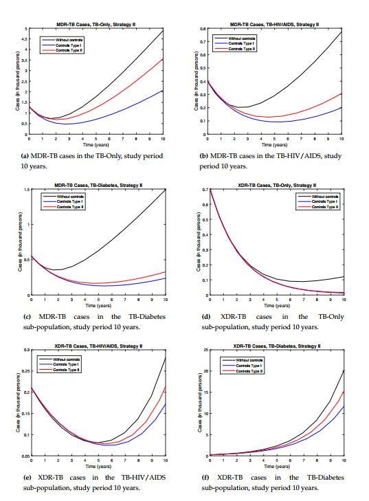
Strategy III. This strategy does not control resistance in the TB-Only sub-population. As in the previous strategies, the objective of reducing resistance in the dynamics is met. Controls in XDR-TB HIV/AIDS and diabetes reduced the number of cases and asymptotic behavior was maintained, but the results were better than strategy II for the different types of controls. This strategy also failed to take advantage of the decrease in the number of cases, reducing the number of cases but not avoiding future asymptotic growth, see Figures 5a, 5e and 5f. Here too, type I controls achieved better results.
In general, all strategies and types of controls met the objective of reducing the number of cases of MDR-TB and XDR-TB. The most efficient strategy was the strategy I with type I control. In addition to significantly reducing the number of cases in all resistance compartments and also takes advantage of the decrease in dynamics and prevents the future growth of cases. In all strategies, type I control showed better results, so it is recommended to start with low control. In [25] the numerical results show the need to reduce XDR-TB in diabetics due to the growth that occurs in this sub-population, so strategy II does not meet significantly this objective. Strategy II is not recommended because it fails to significantly reduce resistance in diabetics and diabetes is a risk factor for adherence to TB treatment.