In this study, we focus on the slip effects on the peristaltic unsteady flow of magnatohydromagnetic Jeffrey fluid in a flow passage with non-conducting and flexible boundary walls. The effect of the magnetic field with varying thermal conductivity is taken under the influence of heat transfer analysis. The dimensionless system of PDEs is solved analytically, and the obtained results are computed for the temperature, pressure drop, the axial pressure gradient, axial velocity, and then these results are discussed for different values of the physical parameters of our interest. For the stream functions, the contour plots are also obtained which indicates the exact flow behavior within the flow channel, and the effects of the physical parameters on Jeffery fluid within the flow channel are discussed briefly. Our results indicate that the heat transfer coefficient decreases with an increase in thermal slip and velocity slip parameters. Furthermore, it shows that the size of the trapped bolus is greater for the inclined magnetic field as compared to the transverse magnetic field.
In magnetohydrodynamics some recent studies [1,2,3,4,5,6,7,8,9,10,11] have considered the peristaltic flow of Newtonian and non-Newtonian fluid and investigated the result of magnetic field on them. Stud et al., [12] investigated the interaction of Poiseuille with peristalsis flow. In an asymmetric tube, the effects of peristalsis of viscous fluid are studied by Mekheimer [13].
In the diagnoses of blood circulation and measurements of blood glucose, the study of heat transfer in blood flow plays a vital role. Our normal blood temperature is about \(37^0\)C, but our proteins start damaging when the temperature is increased from \(41^0\)C.In peristalsis flow, the effect of heat transfer has been investigated by many scholars, but a review of heat transfer by Nadeem and Akbar [14] is quite famous in the era of 2003.
Most of the natural physiological fluids like polymer melts, bubbly fluids, hydrocarbons, and many nuclear aggressive materials are based on complicated stress-strain relations as compared to Newtonian fluids. The governing equations of such fluids give challenges to researchers and scholars. The Jeffrey version of the Oldroyed [15,16,17,18,19,20,21,22] is an important example of non-Newtonian fluid models in which time derivative of strain tensor. Peristaltic action of non-Newtonian fluid for small wave amplitude has been described by Raju and Devanathan [23], the long-wavelength peristalsis analysis is performed by Radhakrishnamacharya [24].
In all the studies mentioned above slip effects in presence of variable thermal conductivity have been ignored. Therefore it is of great interest to study the peristaltic mechanism of hydromagnetic Jeffrey fluid having variable thermal conductivity with slip conditions and we did this analysis because of its practical applications in the field of biomedical engineering and food industries in fluid delivery.
2. Mathematical formulation
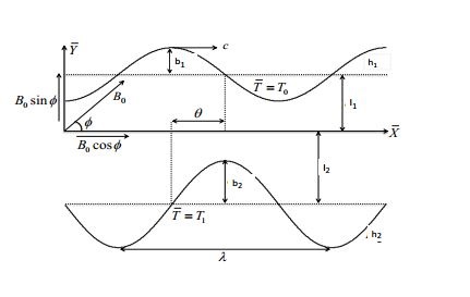
The unsteady flow of an incompressible hydromagnetic fluid in an asymmetric two-dimensional tube having two walls \(\bar{h_1}\) and \(\bar{h_2}\) is considered in this study.
The wall geometries as shown in Figure 1 can be expressed as follows:
where \(\ell_{1}\) and \( \ell_{2}\) are te channel half widths, \(\lambda \) is the wavelength, \(c\) is the wave speed, \(b_{1}\) and \(b_{2}\) are the amplitudes, \(\bar{t}\) is the time, and \(\theta{ }\) is the phase difference. Furthermore, \(\theta\) fulfill the condition
In above equation, \({\bar{\mathbf\nabla}}\) is the gradient operator, and \({\bar{\mathbf V}}=\left[ \bar{U}\left( \bar{X},\bar{Y},\bar{t}\right) ,\bar{V}\left( \bar{X},\bar{Y},\bar{t}\right) ,0\right]\) is the two-dimensional velocity field vector. \({\mathbf{\bar{S}}}\), \({\bar{\mathbf T}}\), and \({\bar{\mathbf I}}\) are respectively the extra stress tensor for Jeffrey fluid, Cauchy stress tensor and the Identity tensor, \(\mathcal{S}_t\) represent the source term, \(c_{p}\) being the specific heat, \(\bar{T}\) is the temperature and \(\mathbf{\bar{q}}\) is the heat flux vector.
The constitution Jeffrey fluid model equations are
where \(\bar{S}\) is extra stress tensor, relaxation time is denoted by \(\lambda _{1}\), fluid viscosity by \(\mu \), and retardation time by \(\lambda _{2}\), \(\bar{P}\) is pressure, and \(\bar{I}\) is the identity tensor.
The components of extra stress tensor \(\mathbf{\bar{S}}\) are
The current density \((\bar{J}= S_{e} \left[ \bar{V}\times \bar{B}_{0}\right])\) where magnetic field under the negligence of impose electric field and induce electric field represent by \(\bar{B}_{0}(=\left[ B_{0}\cos \phi ,B_{0}\sin \phi ,0 \right])\). Thus magnetic body force take the form
In above Eqs (15)-(21), we define the specific heat as \(c_p\), density of the fluid as \(\rho \), and the fluid temperature as \(\bar{T}\); whereas, temperature dependent thermal conductivity \(\bar{\kappa}(\bar{T})\), the viscous dissipation \(\bar{\Phi}_{a}\), and Joule dissipation \(\bar{\Phi}_{b}\) are defined as follows:
where \(\bar{u}\) and \(\bar{v}\) are the respective components of velocity in \(\bar{x}-\)direction and \(\bar{y}-\)directions. Equations (15)-(18) after using equations (20)-(22) give
We define dimensionless pressure \(p\), wave number \(\delta\), Hartman number \(M\), Brinkman number \(\text{Br}\left( =\Pr \times \text{Ec}\right)\), Eckert number \(\text{Ec}\), Prandtl number \(\Pr\), and Reynolds number \(\text{Re}\) as follows:
where \(D_1\), \(D_2\), \(D_3\) and \(D_4\) are constants. The constants are obtained using boundary condition (33).
The axial pressure gradient has been obtained as
Since Eq. (31) is highly non linear, so it is difficult to find the analytical solution. In this study, a perturbation technique has been used to calculate the temperature distribution of Jeffery fluid, so we construct perturbation solution for a small \(\varepsilon\) as
Using Eq. (38) into Eqs (31) and (34) give yield zeroth order and 1st order systems of the temperature distribution, correspondingly. These are given by
This section is aimed to study the slip effects and their importance on a peristaltic mechanism under the influence of different emerging parameters. The graphs have been drawn for various concerned parameters. Note that the values of the parameters are fixed as \(s _{1}=0.75\), \(s _{2}=0.75\), \(\eta=1\), \(\theta =\pi /4\) for all graphs and Tables.
Table 1. \(Z\) (Heat transfer coefficient) as function of \(\phi\) and \(\varepsilon\). Here \(x=0.1\), \(Q=-1.2\), \(M=4\), \(\lambda_{1}=1\), \(\text{Br}=0.5\), \(\beta_1=0.2\), \(\beta_2=0.2\).
\(\phi\)
\(\varepsilon\)
\(\pi /4\)
\(\pi /2\)
\(2 \pi /3\)
\(5 \pi /6\)
\(7 \pi/8\)
\(0.0\)
\(1.6713\)
\(2.41269\)
\(2.04214\)
\(1.29947\)
\(1.14463\)
\(0.1\)
\(1.6961\)
\(2.41624\)
\(2.05731\)
\(1.33195\)
\(1.17971\)
\(0.2\)
\(1.7209\)
\(2.41979\)
\(2.07247\)
\(1.36443\)
\(1.21479\)
Table 2. \(Z\) (Heat transfer coefficient) as function of \(M\) and \(\varepsilon\). Here \(x=0.1\), \(Q=-1.2\), \(\beta_1=0.2\), \(\beta_2=0.2\), \(\phi =\pi /4\), \(\lambda _{1}=1\), \(\text{Br}=0.5\).
\(M\)
\(\varepsilon\)
\(1\)
\(2\)
\(3\)
\(4\)
\(5\)
\(0.0\)
\(0.97064\)
\(1.11242\)
\(1.34606\)
\(1.67129\)
\(2.08847\)
\(0.1\)
\(1.00824\)
\(1.14800\)
\(1.37690\)
\(1.69610\)
\(2.10229\)
\(0.2\)
\(1.04583\)
\(1.18358\)
\(1.40931\)
\(1.72090\)
\(2.11611\)
Table 3. \(Z\) (Heat transfer coefficient) as a function of \(\lambda _{1}\) and \(\varepsilon\). Here \(x=0.1\), \(Q=-1.2\), \(\beta_1=0.2\), \(\beta_2=0.2\), \(\phi =\pi /4\), \(M=4\), \(\text{Br}=0.5\).
\(\lambda_{1}\)
\(\varepsilon\)
\(1\)
\(2\)
\(3\)
\(4\)
\(5\)
\(0.0\)
\(1.67129\)
\(1.65697\)
\(1.64965\)
\(1.64522\)
\(1.64226\)
\(0.1\)
\(1.69610\)
\(1.68210\)
\(1.67496\)
\(1.67063\)
\(1.66774\)
\(0.2\)
\(1.72090\)
\(1.70724\)
\(1.70026\)
\(1.69604\)
\(1.69321\)
Table 4. \(Z\) (Heat transfer coefficient) as a function of \(\text{Br}\) and \(\varepsilon\). Here \(x=0.1\), \(Q=-1.2\), \(\beta_1=0.2\), \(\beta_2=0.2\), \(\phi =\pi /4\), \(M=4\), \(\lambda _{1}=1\).
\(\text{Br}\)
\(\varepsilon\)
\(0.5\)
\(1\)
\(1.5\)
\(2\)
\(2.5\)
\(0.0\)
\(1.67129\)
\(2.45597\)
\(3.24064\)
\(4.02532\)
\(4.80999\)
\(0.1\)
\(1.69610\)
\(2.45803\)
\(3.21107\)
\(3.99555\)
\(4.69048\)
\(0.2\)
\(1.72090\)
\(2.46010\)
\(3.18151\)
\(3.88513\)
\(4.57098\)
Table 5. \(Z\) (Heat transfer coefficient) as a function of \(\beta_1\) and \(\varepsilon\). Here \(x=0.1\), \(Q=-1.2\), \(\beta_2=0.2\), \(Br=0.5\), \(\phi =\pi /4\), \(M=4\), \(\lambda _{1}=1\).
\(\beta_1\)
\(\varepsilon\)
\(0.1\)
\(0.2\)
\(0.3\)
\(0.4\)
\(0.5\)
\(0.0\)
\(1.70382\)
\(1.67129\)
\(1.65603\)
\(1.64778\)
\(1.64275\)
\(0.1\)
\(1.72792\)
\(1.69610\)
\(1.68124\)
\(1.67313\)
\(1.66822\)
\(0.2\)
\(1.75196\)
\(1.72090\)
\(1.70640\)
\(1.69848\)
\(1.69368\)
Table 6. \(Z\) (Heat transfer coefficient) as a function of \(\beta_2\) and \(\varepsilon\). Here \(x=0.1\), \(Q=-1.2\), \(\beta_1=0.2\), \(Br=0.5\), \(\phi =\pi /4\), \(M=4\), \(\lambda _{1}=1\).
\(\beta_2\)
\(\varepsilon\)
\(0.1\)
\(0.2\)
\(0.3\)
\(0.4\)
\(0.5\)
\(0.0\)
\(1.73194\)
\(1.67129\)
\(1.61795\)
\(1.57066\)
\(1.52845\)
\(0.1\)
\(1.76865\)
\(1.69610\)
\(1.63254\)
\(1.57635\)
\(1.52629\)
\(0.2\)
\(1.80537\)
\(1.72090\)
\(1.64713\)
\(1.58205\)
\(1.52414\)
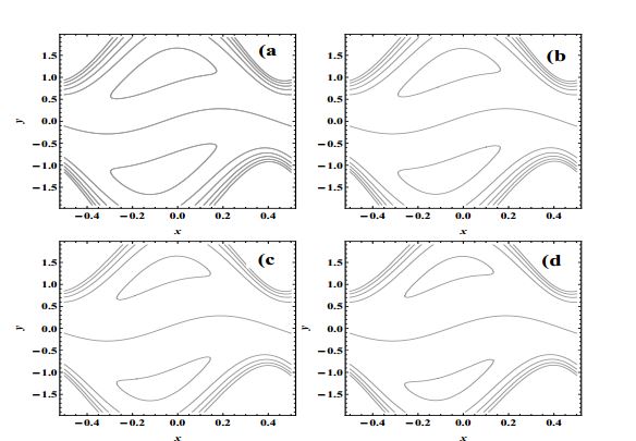
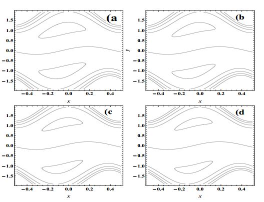
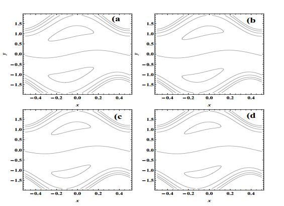
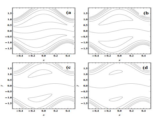
Figure 6. Effect on trapping by \(\phi \) with \(Q=1.48\), \(M=1.2\), \(\lambda_{1}=1\), (a); \(\phi\)=0,\,(b); \(\phi=\pi/6\),\,(c); \(\phi=\pi/3\),\,(d); \(\phi=\pi/2\).Figure 7. Effect on trapping by \(M\) with \(Q=1.48\), \(\phi =\pi /4\), \(\lambda _{1}=1\)(a); \(M\)=0,\,(b); \(M\)=1,\,(c); \(M\)=1.3,\,(d); \(M\)=1.5\,.Figure 8. Influence of \(\lambda _{1}\) on trapping with \(Q=1.48\), \(\phi =\pi /4\), \(M=1\)\, (a); \(\lambda_1\)=0,\,(b); \(\lambda_1\)=2,\,(c); \(\lambda_1\)=3,\,(d); \(\lambda_1\)=4.Figure 9. Effect on trapping by \(\lambda _{1}\) with \(Q=1.48\), \(\phi =\pi /4\), \(M=1\), \(\lambda _{1}=1\) \, (a); \(\beta_1\)=0,\,(b); \(\beta_1\)=0.1,\,(c); \(\beta_1\)=0.2,\,(d); \(\beta_1\)=0.3,\,.
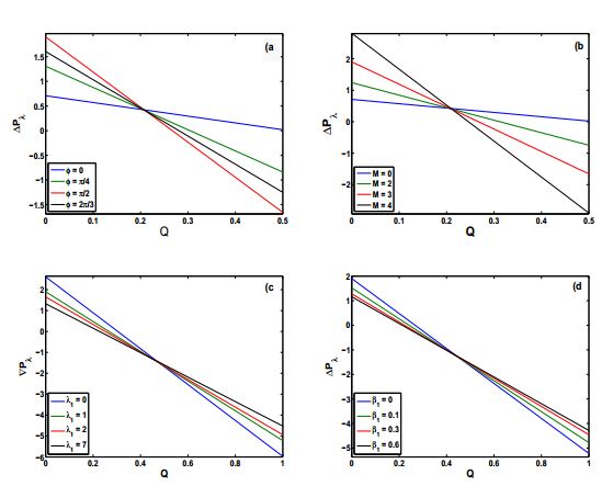
The variation of pressure drop per wavelength \(\Delta P_{\lambda }\) verses flow rate \(Q\) is shown in Figure 2. Influence of inclination angle \(\phi\) on pressure drop \(\Delta P_{\lambda}\) is depicted in Figure 2(a). It is observed that In the peristaltic pumping region, the pumping rate starts increasing when \(\phi\) is increased from \(0\) to \(\pi/2\); whereas it decreases in the augmented pumping region. It shows opposite behavior for \(\phi \in [0,\pi/2]\) .
Figure 2(b) give us opportunity to study the connection between Hartman number \(M\) and \(\Delta P_{\lambda }\). In the positive feasible solution area which is the peristaltic pumping area, a rise in pressure drop is observed as we increase Heartman number \(M\). In the augmented pumping region action of pumping performance remains increasing.
Figure 2(c) is papered to investigate the behavior on \(\Delta P_{\lambda }\) by Jeffrey fluid parameter \(\lambda _{1}\) . It is seen that the pumping rate under the effects of \(\lambda _{1}\) shows increasing behavior.
Figure 2(d) illustrate the effects of thermal slip parameter \(\beta _{1}\) on \(\Delta P_{\lambda }>0\). It is seen that the pumping rate under the effects of \(\lambda _{1}\) shows increasing behavior.
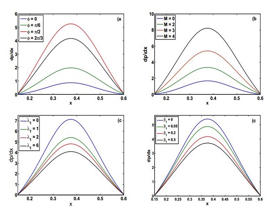
Figure 3 shows the pressure gradient profile for one wavelength. It illustrates that in the wider part of channel \(x\in [0,0.2]\) and \(x\in[0.65,1]\) the flow can pass easily without implementation of a large pressure gradient, that’s why pressure gradient is small in that region, but in the narrow part of the channel \(x\in[0.3,0.6],\) flow can pass with same flux under the large pressure gradient, especially the narrowest position \(x=0.45\). This phenomenon is well in accordance with the physical situation. We also observe the effect of \(\phi\), \( M \), \( \lambda_1 \) and \( \beta_1 \) on \(dp/dx\) by using fixed values of other parameters. The amplitude of \(dp/dx\) increases with increase in values of \(\phi\) and \(M\) while it decrease as \( \lambda_1 \) and \(\beta_1 \) increases.
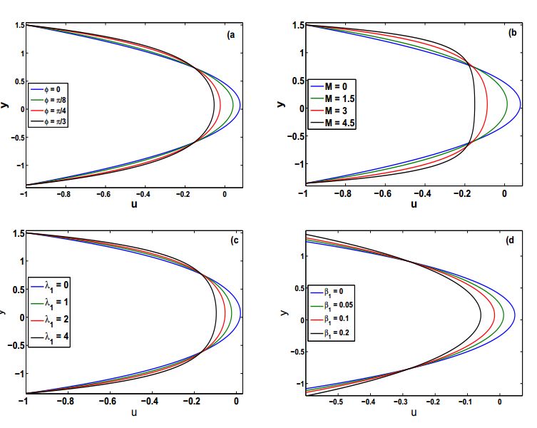
The velocity profile for different parameters is shown in Figure 4. We observe that the velocity profile shows decreasing behavior for a gradually increase in \(\phi\), \(M\), \(\lambda_1\) and \(\beta_1\).
5.2. Heat transfer characteristics
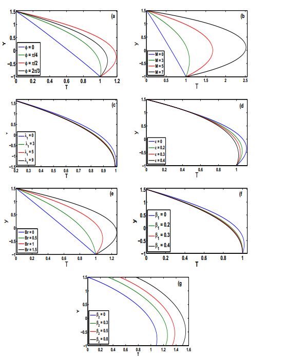
Figure 5 shows the variation of fluid temperature for various parameters. After examining Figure 5 we concluded that, if \(\phi\) is raised from \(0\) to \(\pi/2\) then temperature increases. As \(\phi\) is raised from \(\pi/2\) to \(\pi\) then temperature decreases. When Heartman number \(M\) is increased then the temperature is also increased, while an increase in \(\lambda _{1}\) the temperature shows decreasing behavior. Under the effects of viscous and Joule dissipation, the temperature got increases with an increase in \(Br\). An increase in thermal slip parameters and velocity slip parameter temperature shows decreasing behavior.
Tables 1-6 give us the numerical results of heat transfer coefficient \(Z\) various parameters. From Table 1, we observe that the heat transfer coefficient is less for hydrodynamic fluid but large for the hydromagnetic fluid.
The value of the heat transfer coefficient \(Z\) increases under the effect of \(\phi \in \left[ 0,\pi /2\right] \); however, opposite behavior is observed for \(\phi \in \left[ \pi /2,\pi\right]\). Table 2 tells us that the value of \(Z\) increases as we move from Jeffrey fluid to Newtonian fluid. Table 4 witness that the heat transfer coefficient \(Z\) increases under the consideration of the viscous and Joule dissipation.
Table 5 and Table 6 tell us that the heat transfer coefficient \(Z\) decreases as we increase thermal slip parameters and velocity slip parameters.
5.3. Trapping phenomena
The plots for streamlines for different values of \(M\), \(\phi\), \(\beta_1\), \(\beta_2\) and \(\lambda _{1}\) are given in Figures 6-8. Figure 6 depicts that size of trapped bolus reduces as a result of increasing \(\phi \in [0,\pi /2]\); however, the situation is reversed for \(\phi \in [\pi /2, \pi]\), it displays an inverse behavior. Figure 7 concludes that the trapped bolus is smaller in size for hydromagnetic fluids than hydrodynamic fluids. It can be seen from Figure 8 that the size of the bolus is a decreasing function of Jeffrey fluid parameter \(\lambda_1\). Figure 9 tells us that the size of the trapped bolus falls down with an increment in the value of velocity slip parameter \(\beta_1\).
6. Concluding remarks
The peristaltic flow of a hydromagnetic Jeffrey fluid under the influence of an inclined magnetic field and variable thermal conductivity with slip conditions has been analyzed. The influence of various parameters is discussed graphically. The main finding can be summerize as listed below.
The magnetic field for\(\phi \in \left[ 0,\pi /2\right]\) shows opposite behavior when compared with \(\phi \in \left[ \pi /2,\pi \right] \).
For magnetic fluid, the value of axial pressure gradient is higher rather than Newtonian fluid.
An increase in \(\phi\) and \(M\) leads to an increase in \(dp/dx\), whilst it decreases when \(\lambda _{1}\) is increased.
The magnitude of \(dp/dx\) show decreasing behavior when \(\beta_1\) is increased.
The amplitude of velocity \(u\) is a decreasing function of \(\phi \in \left[ 0,\pi /2\right]\) , \( \beta_1\), \(M\) and \(\lambda _{1}\).
The temperature of the fluid \(T\) falls down under the effect of \(\phi \in \left[ 0,\pi/2 \right]\); Contrarily, it decreases with an increase in conductivity parameter \(\varepsilon .\)
Ascending values of \(\lambda _{1}\) decreases the value of heat transfer coefficient \(Z\), whilst, an increment in the values of \(M,\) \(\varepsilon \) and \( \text{Br}\) leads to an increase in heat transfer coefficient \(Z\).
The heat transfer coefficient decreases as we increase thermal slip parameters \(\beta_2\) and velocity slip parameter \(\beta_1\).
Size of the trapped bolus is greater for the inclined magnetic field as compared with the transverse magnetic field. Moreover, increasing \(M\), \(\beta_1\), and \(\lambda _{1}\) decreases the size of the trapped bolus.
Appendix
Here we include the values of \(D_i(i=1,2,….,11)\) and \(R_i(i=1,2,.. ,26)\).
\begin{equation*} \label{chap4-conR-sai}
\begin{aligned}
&R_1=8 (h_1+h_2)\sqrt{1+\lambda_1 } ,\\
&R_2=\frac{R_1}{2}(-2-F M^2 \beta_1 (1+\lambda_1 ) + F M^2 \beta_1 (1+\lambda_1 )\cos2\phi){\cosh}((h_1-h_2)M\sqrt{1+\lambda_1}\sin\phi),\\
&R_{3a}=M(1+\lambda_1)2(h_1+h_2)(-4\beta_1-F(2+M^2\beta1^2(1+\lambda_1),\\
&R_{3b}=F M^2 \beta_1^2 (1+\lambda_1 ) \cos 2\phi \sin\phi \sinh( M (\sqrt{1+\lambda_1})(h_1-h_2)\sin\phi)),\\
&R_4=-16 \sqrt{1+\lambda_1},\\
&R_{5a}=8\sqrt{1+\lambda_1} (2- M^2 \beta_1 (h_1-h_2)(1+\lambda_1 )+
(h_1-h_2) M^2 \beta_1 (1+\lambda_1 ),\\
&R_{5b}=\cos 2\phi\cosh( M \sqrt{1+\lambda_1 } \sin\phi (h_1-h_2)) ,\\
&R_{6a}=8M (1+\lambda_1 ) \sin\phi (h_1-h_2-2 \beta_1,\\
&R_{6b}=(h_1-h_2) M^2 \beta_1^2 (1+\lambda_1 )\sin \phi ^2\sinh ( M \sqrt{1+\lambda_1} \sin \phi (h_1-h_2))),\\
&R_7= \cosh (h_{1} M \sqrt{1+\lambda_1} \sin \phi ) \sin \phi ,\\
&R_8=F M \sqrt{1+\lambda_1} \cosh(h2 M \sqrt{1+\lambda_1} \sin\phi) F M \sqrt{1+\lambda_1 }\sin\phi ,\\
&R_9=(2+F M^2 \beta_1 (1+\lambda_1) \sin\phi^2),\\
&R_{10}=\sinh ( \sqrt{1+\lambda_1}h1 M \sin\phi)-\sinh( \sqrt{1+\lambda_1} \sin \phi h2 M),\\
&R_{11}= \cosh(h1 M \sqrt{1+\lambda_1} \sin\phi) \sin \phi,\\
&R_{12}=(h1-h2) M \sqrt{1+\lambda_1} \cosh(h2 M \sqrt{1+\lambda_1} \sin\phi) (h1-h2) M \sqrt{1+\lambda_1}\sin \phi,\\
&R_{13}=-2+(h1-h2) M^2 \beta 1 (1+\lambda_1) \sin\phi^2,\\
&R_{14}=\sinh( \sin\phi h1 M \sqrt{1+\lambda_1})-\sinh( \sqrt{1+\lambda_1}h2 M \sin\phi),\\
&R_{15}= \cosh(h_1 M \sqrt{1+\lambda_1}\sin \phi)(F+h_1-h_2) \sqrt{1+\lambda_1},\\
&R_{16}= \cosh(h_2 M \sqrt{1+\lambda_1}\sin \phi)(F+h_1-h_2),\\
&R_{17}=(F+h_1-h_2)M \beta_1 (1+\lambda_1)\sin\phi \sinh(h_1 M \sqrt{1+\lambda_1}\sin \phi),\\
&R_{18}=(F+h_1-h_2)M \beta_1 (1+\lambda_1)\sin\phi \sinh(h_2 M \sqrt{1+\lambda_1}\sin \phi),\\
&R_{19}=(h_1-h_2) M^2 \beta_1({1+\lambda_1}^3/2 +(1+\lambda_1)\cos2\phi),\\
&R_{20}=\cosh(\sqrt{1+\lambda_1}\sin \phi (h_1-h_2) M ),\\
&R_{21}=(h_1-h2)\sin\phi(2\beta_1+M^2 \beta_1^2(1+\lambda_1)\sin\phi^2)M(1+\lambda_1),\\
&R_{22}=\sinh(h_1-h_2 M \sqrt{1+\lambda_1}\sin \phi),\\
&R_{23}=\sin\phi\beta_1 {1+\lambda_1} \cosh(h_1 M \sqrt{1+\lambda_1}\sin \phi)(F+h_1-h_2) M (F+h_1-h_2) M ,
\end{aligned}
\end{equation*}
\begin{equation*}\label{chap4-conR1-sai}
\begin{aligned}
&R_{24}=\sin\phi \cosh(h_2 M \sqrt{1+\lambda_1}\sin \phi)(F+h_1-h_2),\\
&R_{25}= \sqrt(1+\lambda_1)\sinh(h_1 M \sqrt{1+\lambda_1}\sin \phi)(F+h_1-h_2),\\
&R_{26}=\sinh(h_2 M \sqrt{1+\lambda_1}\sin \phi)\sqrt(1+\lambda_1)(F+h_1-h_2) ,\\
&D_1=-\frac{R_1+R_2+R_{3a}+R_{3b}}{R_4+R_{5a}+R_{5b}-R_{6a}-R_{6b}},\\
&D_2=\frac{R_7+R_8+R_9 R_{10}}{R_{11}+R_{12}+R_{13} R_{14}},\\
&D_3=-\frac{R_{15}-R_{16}+R_{17}+R_{18}}{(R_{19}R_{20}-R_{21}R_{22})},\\
&D_4=\frac{R_{23}+R_{24}+R_{25}-R_{26}}{(R_{19}R_{20}-R_{21}R_{22})},\\
&D_5=2(F+h_1-h_2)M^3 \cosh((h_1-h_2) M \sqrt{1+\lambda_1}\sin \phi)\sin\phi^3,\\
&D_6=\sqrt{1+\lambda_1}\cosh(\frac{1}{2}(h_1-h_2) M \sqrt{1+\lambda_1}\sin \phi),\\
&D_7=M \beta_1 {1+\lambda_1}\sin\phi\sinh(\frac{1}{2}(h_1-h_2) M \sqrt{1+\lambda_1}\sin \phi),\\
&D_8=\frac{-1+f_{0}(x,h_2)+f_{0}(x,h_1)+\beta_{2}\left( f\prime_{0} (x,h_2)+ f\prime_{0}(x,h_1) \right)}{2\beta_2 +h_1 +h_2},\\
&D_9=\frac{\beta_2+h_1+f_{0}(x,h_1)(\beta_2+h_2) +f_{0}(x,h_2)(\beta_2+h_1)-\beta_{2}(\beta_2+h_1)\left( f\prime_{0} (x,h_2)\right)}{2\beta_2 +h_1 +h_2}\\
&\quad +\frac{ f\prime_{0}(x,h_1)(2\beta_{2}^2+\beta_2 h_1 +\beta_2 h_2 -\beta_2 – h_1)}{2\beta_2 +h_1 +h_2},\\
&D_{10}=\frac{-f_{1}(x,h_2)+f_{1}(x,h_1)+\beta_{2}\left( f\prime_{1} (x,h_2)+ f\prime_{1}(x,h_1) \right)}{2\beta_2 +h_1 -h_2},\\
&D_{11}= \frac{-f_{1}(x,h_1)(-1+2 \beta_2 +h_1 – h_2 )+f_{1}(x,h_2)+(f_{1}(x,h_2)}{2\beta_2 +h_1 -h_2 } \\
&\quad -\frac{f\prime_{1}(x,h_1)(\beta_2 h_1-\beta_2 h_2 + 2\beta_2^2 +\beta_2)+ f\prime_{1}(x,h_2) }{2\beta_2 +h_1 -h_2}.
\end{aligned}
\end{equation*}
Conflicts of Interest:
The authors declare that they have no conflict of interest.
Data Availability:
All data required for this research is included in this paper.
Funding Information:
No funding is available for this research.
Author Contributions:
Z.A. developed the theoretical formalism and performed the analytic calculations and numerical and graphical simulations. S.T. and R.A. contributed to the final version of the manuscript. All authors read and approved the final version of the manuscript.
References
Ali, N., Hayat, T., & Sajid, M. (2007). Peristaltic flow of a couple stress fluid in an asymmetric channel. Biorheology, 44(2), 125-138. [Google Scholor]
El Misiery, A. E. M. (2002). Effects of an endoscope and generalized Newtonian fluid on peristaltic motion. Applied Mathematics and Computation, 128(1), 19-35. [Google Scholor]
Sobamowo, M. G., Kamiyo, O. M., Yinusa, A. A., & Akinshilo, T. A. (2020). Magneto-squeezing flow and heat transfer analyses of third grade fluid between two disks embedded in a porous medium using Chebyshev spectral collocation method. Open Journal of Mathematical Sciences, 4, 305-322. [Google Scholor]
Hayat, T., Kara, A. H., & Momoniat, E. (2003). Exact flow of a third-grade fluid on a porous wall. International Journal of Non-Linear Mechanics, 38(10), 1533-1537. [Google Scholor]
Misra, S., Narender, G., & Govardha, K. Numerical solution of boundary layer flow of MHD nanofluid over a stretching surface with chemical reaction and viscous dissipation effects. Open Journal of Mathematical Sciences, 3, 289 – 299[Google Scholor]
Fetecau, C., & Fetecau, C. (2005). Starting solutions for some unsteady unidirectional flows of a second grade fluid. International Journal of Engineering Science, 43(10), 781-789. [Google Scholor]
Hayat, T., & Kara, A. H. (2006). Couette flow of a third-grade fluid with variable magnetic field. Mathematical and Computer Modelling, 43(1-2), 132-137. [Google Scholor]
Khalique, C. M., Safdar, R., & Tahir, M. (2019). First analytic solution for the oscillatory flow of a Maxwells fluid with annulus. Open Journal of Mathematical Sciences, 2, 1-9. [Google Scholor]
Farooq, M. U., Khan, M. S., & Hajizadeh, A. (2019). Flow of viscous fluid over an infinite plate with Caputo-Fabrizio derivatives. Open Journal of Mathematical Sciences, 3, 115-120. [Google Scholor]
Ali, N., & Hayat, T. (2007). Peristaltic motion of a Carreau fluid in an asymmetric channel. Applied Mathematics and Computation, 193(2), 535-552. [Google Scholor]
Ferraro, V. C., & Plumpton, C. (1966). Introduction to Magneto-Fluid Mechanics, 2nd Edition. Clarendon Press, Oxford. [Google Scholor]
Stud, V. K., Sephon, G. S., & Mishra, R. K. (1977). Pumping action on blood flow by a magnetic field. Bulletin of Mathematical Biology, 39(3), 385-390. [Google Scholor]
Mekheimer, K. S. (2004). Peristaltic flow of blood under effect of a magnetic field in a non-uniform channels. Applied Mathematics and Computation, 153(3), 763-777. [Google Scholor]
Nadeem, S., & Akbar, N. S. (2009). Peristaltic flow of a Jeffrey fluid with variable viscosity in an asymmetric channel. Zeitschrift für Naturforschung A, 64(11), 713-722. [Google Scholor]
Oldroyd, J. G. (1950). On the formulation of rheological equations of state. Proceedings of the Royal Society of London. Series A. Mathematical and Physical Sciences, 200(1063), 523-541. [Google Scholor]
Larson, R. G. (2013). Constitutive Equations for Polymer Melts and Solutions: Butterworths series in chemical engineering. Butterworth-Heinemann. [Google Scholor]
Rajagopal, K. R. (1993). Mechanics of non-Newtonian fluids. Pitman Research Notes in Mathematics Series, 129-129. [Google Scholor]
Afsar Khan, A., Ellahi, R., & Vafai, K. (2012). Peristaltic transport of a Jeffrey fluid with variable viscosity through a porous medium in an asymmetric channel. Advances in Mathematical Physics, 2012, Article ID 169642. https://doi.org/10.1155/2012/169642. [Google Scholor]
Hayat, T., Javed, M., & Ali, N. (2008). MHD peristaltic transport of a Jeffery fluid in a channel with compliant walls and porous space. Transport in Porous Media, 74(3), 259-274. [Google Scholor]
Kothandapani, M., & Srinivas, S. (2008). Peristaltic transport of a Jeffrey fluid under the effect of magnetic field in an asymmetric channel. International Journal of Non-Linear Mechanics, 43(9), 915-924. [Google Scholor]
Pandey, S. K., & Tripathi, D. (2010). Unsteady model of transportation of Jeffrey-fluid by peristalsis. International Journal of Biomathematics, 3(04), 473-491. [Google Scholor]
Vajravelu, K., Sreenadh, S., & Lakshminarayana, P. (2011). The influence of heat transfer on peristaltic transport of a Jeffrey fluid in a vertical porous stratum. Communications in Nonlinear Science and Numerical Simulation, 16(8), 3107-3125. [Google Scholor]
Raju, K. K., & Devanathan, R. (1972). Peristaltic motion of a non-Newtonian fluid. Rheologica Acta, 11(2), 170-178. [Google Scholor]
Radhakrishnamacharya, G. (1982). Long wavelength approximation to peristaltic motion of a power law fluid. Rheologica Acta, 21(1), 30-35. [Google Scholor]