Using the Kudryashov and Tanh methods, we have obtained novel exact solutions for the Paraxial Wave Dynamical Equation with Kerr law, including various types of wave solutions. These distinct types of wave solutions have important applications in physics and engineering, and their physical characteristics are well defined. These outcomes are a substantial innovation in the study of water waves in mathematical physics and engineering phenomena. The results we have acquired demonstrate the power and effectiveness of the present techniques.
Keywords: Kudryashov method; Optical solitons; Paraxial wave dynamical model with Kerr law non-linearity; Tanh method.
1. Introduction
Nonlinear phenomena are an essential area of research that arises in several branches of engineering and physical sciences, including plasma, solid-state physics, optical fibers, chemical kinetics, biology, and fluid mechanics. Nonlinear evolution equations (NLEEs) often play a crucial role in the mathematical representation of these phenomena. Obtaining the solutions of NLEEs can aid in understanding the dynamics of these phenomena. Exact traveling wave solutions (TWSs) of NLEEs have become increasingly important tools in physical phenomena.
Various methods have been used to obtain TWSs for NLEEs in previous works, such as the new extended direct algebraic method [1, 2, 3], the first integral method [4, 5], the generalized Kudryashov method [6, 7], the new extended hyperbolic function method [8], the undetermined coefficient method, and modified mapping method [9], the extended simple equation methods [10], the Jacobi elliptic functions method [11,12], Kudryashov’s methods [13, 14], the generalized tanh method (GTM) [15], the exp-function method [16], the auxiliary equation method and Sine-Cosine method [17], the mapping method [18], the Exp \((-f(e))\)-expansion method [19], the modified simple equation method [20], the generalized \((G’/G)\) expansion method [21]25}, the modified Khater method [22, 23], the extended \((G’/G)\)-expansion method [24, 25], the homotopy perturbation double Sumudu transform method [26], the tan method, and the tanh method [27], the fractional extended Fan sub-equation method [28], and the modified auxiliary equation method [33,34], and the sub-equation method [29, 30].
In this paper, we focus on constructing novel exact solutions of the Paraxial Wave Dynamical Equation with Kerr law using the Kudryashov and Tanh methods. Our solutions include multiple types of wave solutions, which have important applications in physics and engineering. The physical characteristics of these solutions are well-defined, and the results demonstrate the power and effectiveness of the present techniques.
The paper is structured as follows: S2 presents the governing equation, while S3 discusses the proposed analysis method. In S4, we apply the Kudryashov method, while S5 presents the analysis and application of the tanh method. Finally, we provide the conclusion of this paper in S6.
2. Governing model
Using Kerr media, the dimensionless time-dependent Paraxial wave
equation (PWE) [31] through
limiting the diffraction into one-dim in the existence of GVD is
given as,
here, \(E\) represents the addition of complex waves, the \(t\), ~\( y\),~
and~ \(z\) represent temporal, spatial and longitudinal promulgation
veriables, correspondingly. In Eq.
(\ref{eq1}), \(\beta,~ \gamma, ~ and~
\alpha\) are real numbers and denote the effects of diffraction,
non-linearity of Kerr and dispersal, similarly. Eq.
(\ref{eq1}) convert into hyperbolic NLSE
if \(\alpha \beta < 0\) and its convert into elliptic NLSE
[32] if \(\alpha \beta
> 0\). Clearly, this model can also describe (2+1)- dim dynamic of
spatial in cubic-Kerr media, disregarding GVD, in this sense\(y,~t\)
represent the coordinates of temporal and spatial transverse and z
denotes the longitudinal coordinate. Moreover \(\alpha = \beta~> 0\),
where \(f_0\) and \(f_1\) are constants. Substituting Eq.
(\ref{eq13}) into Eq.
(\ref{eq3}), corresponding the coefficients
of \(Q(\eta)\) to zero, gets a set of equations. On solving the
system, the \(f_j,~ j=0,1,2,3\)
are achieved novel sets of solution for Eq. (\ref{eq1}).
5. Description of the generalized tanh method [15]
Let PDE as given in (\ref{eq1}) with the
wave transformation in
(\ref{eq2}) and (\ref{eq3})
using wave transformation ODE is obtained as in
(\ref{eq4}). We assume that
(\ref{eq4}) has a solution, as
By using balancing rule in (\ref{eq4}) the
value of \(N\) is found. Replacing
(\ref{eq20}) into
(\ref{eq4}) with
(\ref{eq21}), gives a set of equations for
\(f_j(j = (0, 1,2, 3, ….N))\). On solving this set,
we yield set of solutions that admits (\ref{eq4}), as follows
Consider the solutions of (\ref{eq21}) are, as
Putting (\ref{eq27}) and
(\ref{eq21}) in
(\ref{eq4}) produces a polynomial in form
of \(Q(\eta)\). We get a system on making a comparison of the coefficients of \(Q(\eta)\) to zero, after solving it we get solutions as
Set 1
\(f_0=0\),~~~\(f_1=\frac{\sqrt{-\alpha w^2-\beta
k_1^2}}{\gamma}\),~\(\mu_2=-\frac{\alpha \tau^2}{2}+h\alpha w^2+h\beta
k_1^2-\frac{\beta
\mu_1^2}{2}.\)
If \(h<0\), then
The results of this paper will be valuable for researchers to study
the most noticeable applications of the paraxial dynamical model
with Kerr law non-linearity in optic fibers. Figures 1-5
reveals the surfaces of the solution acquired for 3-D and 2-D plots,
with a selection of suitable parameters for the paraxial dynamical
model with Kerr law non-linearity. Likewise, 3D plots provide us to
model and exhibit correct physical behavior. Through this study, we
consider the optical soliton solutions to the nonlinear paraxial
dynamical model with Kerr law non-linearity using the Kudryashov and tanh methods.
The authors proposed different analytic approaches in
the newly issued article and reported some fascinating findings. The
author can understand from all the graphs that the proposed methods
are very effective and more specific in assessing the equation under
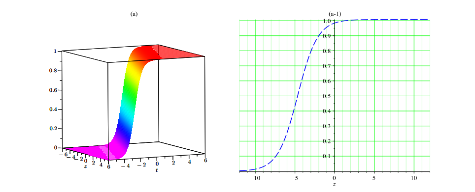
consideration. Figure 1 indicates the solution given by (\ref{eq16}), which
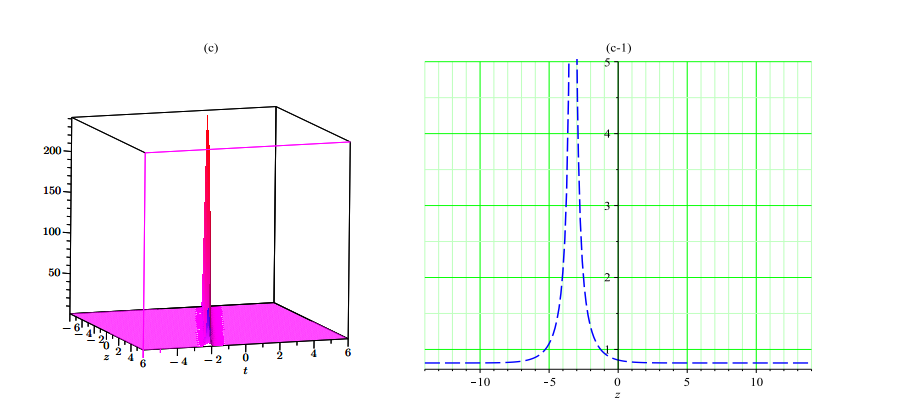
is dark. Figures 2 and 3 indicate the solutions given by (\ref{eq28}) and
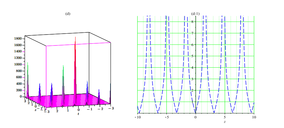
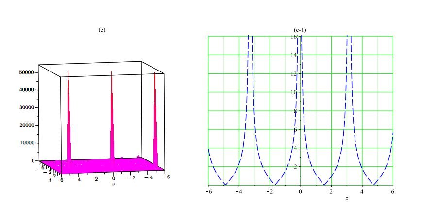
(\ref{eq29}), which are dark and singular, respectively. Figures 4 and 5 are
the graphical representations of the solutions given by (\ref{eq36}) and
(\ref{eq37}), which are periodic singular solitons.
7. Conclusion
In this work, we have successfully obtained exact solutions of the paraxial dynamical model with Kerr law non-linearity using the Kudryashov and Tanh methods. These results are of great significance in the study of physical phenomena such as optics and optical fibers, as they can help to better understand the behavior of non-linear optic systems and provide a foundation for future research.
Both the Kudryashov and Tanh methods employed in this study have demonstrated their consistency, efficiency, and effectiveness in solving non-linear PDEs. These methods can be utilized to develop new exact solitons and deepen our understanding of complex physical systems.
The exact solutions obtained in this study have the potential to be applied in a wide range of physical phenomena beyond optics and optical fibers. The Kudryashov and Tanh methods can be adapted and employed in other fields of research, such as fluid mechanics, plasma physics, and quantum mechanics, where non-linear PDEs are frequently encountered.
Overall, the results of this work demonstrate the power and applicability of the Kudryashov and Tanh methods in solving non-linear PDEs and provide a foundation for future research in various fields of physics.
Figure 1. 3-d plot of (16) (left) and (a-1) 2-d plot of (16) with \(t=1\) (right).Figure 2. 3-plot of (28) (left) and (b-1) 2-plot of (28) with \(t=1\) (right).Figure 3. 3-d plot of (29) (left) and (c-1) 2-d plot of (29) with \(t=1\) (right).Figure 4. 3-d graph of (36) (left) and (d-1) 2-d plot of (36) with \(t=1\) (right).Figure 6. 3-d graph of (37) (left) and (e-1) 2-d plot of (37) with \(t=1\) (right).
Conflicts of Interest:
The authors declare no conflict of interest.
References
Ur Rehman, H., Asjad Imran, M., Ullah, N., & Akgül, A. (2021). On solutions of the Newell–Whitehead–Segel equation and Zeldovich equation. Mathematical Methods in the Applied Sciences, 44(8), 7134-7149.[Google Scholor]
Rehman, H. U., Ullah, N., & Imran, M. A. (2021). Optical solitons of Biswas-Arshed equation in birefringent fibers using extended direct algebraic method. Optik, 226, 165378.[Google Scholor]
Rehman, H. U., Ullah, N., Asjad, M. I., & Akgül, A. (2020). Exact solutions of convective–diffusive Cahn–Hilliard equation using extended direct algebraic method. Numerical Methods for Partial Differential Equations, 2020, 1–16. [Google Scholor]
Raza, N., Arshed, S., & Sial, S. (2019). Optical solitons for coupled Fokas–Lenells equation in birefringence fibers. Modern Physics Letters B, 33(26), 1950317.[Google Scholor]
Arshed, S., & Raza, N. (2020). Optical solitons perturbation of Fokas-Lenells equation with full nonlinearity and dual dispersion. Chinese Journal of Physics, 63, 314-324.[Google Scholor]
Awan, A. U., Rehman, H. U., Tahir, M., & Ramzan, M. (2021). Optical soliton solutions for resonant Schrödinger equation with anti-cubic nonlinearity. Optik, 227, 165496.[Google Scholor]
Tahir, M., Kumar, S., Rehman, H., Ramzan, M., Hasan, A., & Osman, M. S. (2021). Exact traveling wave solutions of Chaffee–Infante equation in (2+ 1)-dimensions and dimensionless Zakharov equation. Mathematical Methods in the Applied Sciences, 44(2), 1500-1513.[Google Scholor]
Rehman, H. U., Imran, M. A., Ullah, N., & Akgül, A. (2020). Exact solutions of (2+1)-dimensional Schrödinger’s hyperbolic equation using different techniques. Numerical Methods for Partial Differential Equations, 2020, 1-20. [Google Scholor]
Rehman, H. U., Younis, M., Jafar, S., Tahir, M., & Saleem, M. S. (2020). Optical solitons of biswas-arshed model in birefrigent fiber without four wave mixing. Optik, 213, 164669.[Google Scholor]
Sultan, A. M., Lu, D., Arshad, M., Rehman, H. U., & Saleem, M. S. (2020). Soliton solutions of higher order dispersive cubic-quintic nonlinear Schrödinger equation and its applications. Chinese Journal of Physics, 67, 405-413.[Google Scholor]
Zubair, A., & Raza, N. (2019). Bright and dark solitons in (n+ 1)-dimensions with spatio-temporal dispersion. Journal of Optics, 48(4), 594-605.[Google Scholor]
Raza, N., & Zubair, A. (2018). Bright, dark and dark-singular soliton solutions of nonlinear Schrödinger’s equation with spatio-temporal dispersion. Journal of Modern Optics, 65(17), 1975-1982.[Google Scholor]
Rehman, H. U., Jafar, S., Javed, A., Hussain, S., & Tahir, M. (2020). New optical solitons of Biswas-Arshed equation using different techniques. Optik, 206, 163670.[Google Scholor]
Rehman, H. U., Ullah, N., & Imran, M. A. (2019). Highly dispersive optical solitons using Kudryashov’s method. Optik, 199, 163349.[Google Scholor]
Ullah, N., Rehman, H. U., Imran, M. A., & Abdeljawad, T. (2020). Highly dispersive optical solitons with cubic law and cubic-quintic-septic law nonlinearities. Results in Physics, 17, 103021. [Google Scholor]
Awan, A. U., Tahir, M., & Rehman, H. U. (2020). Singular and bright-singular combo optical solitons in birefringent fibers to the Biswas-Arshed equation. Optik, 210, 164489.[Google Scholor]
ur Rehman, H., Tahir, M., Bibi, M., & Ishfaq, Z. (2020). Optical solitons to the Biswas–Arshed model in birefringent fibers using couple of integration techniques. Optik, 218, 164894. [Google Scholor]
Rehman, H. U., Saleem, M. S., Zubair, M., Jafar, S., & Latif, I. (2019). Optical solitons with Biswas–Arshed model using mapping method. Optik, 194, 163091. [Google Scholor]
Raza, N., Abdullah, M., & Butt, A. R. (2018). Analytical soliton solutions of Biswas–Milovic equation in Kerr and non-Kerr law media. Optik, 157, 993-1002.[Google Scholor]
Raza, N., & Javid, A. (2019). Dynamics of optical solitons with Radhakrishnan–Kundu–Lakshmanan model via two reliable integration schemes. Optik, 178, 557-566.[Google Scholor]
Awan, A. U., Tahir, M., & Rehman, H. U. (2019). On traveling wave solutions: The Wu–Zhang system describing dispersive long waves. Modern Physics Letters B, 33(6), 1950059. [Google Scholor]
Khater, M., Park, C., Lu, D., & Attia, R. A. (2020). Analytical, semi-analytical, and numerical solutions for the Cahn–Allen equation. Advances in Difference Equations, 2020, 9. [Google Scholor]
Khater, M. M., Attia, R. A., & Lu, D. (2020). Computational and numerical simulations for the nonlinear fractional Kolmogorov–Petrovskii–Piskunov (FKPP) equation. Physica Scripta, 95(5), 055213. [Google Scholor]
Tahir, M., Awan, A. U., & Rehman, H. U. (2019). Optical solitons to Kundu–Eckhaus equation in birefringent fibers without four-wave mixing. Optik, 199, 163297. [Google Scholor]
Tahir, M., Awan, A. U., & Rehman, H. U. (2019). Dark and singular optical solitons to the Biswas-Arshed model with Kerr and power law nonlinearity. Optik, 185, 777-783.[Google Scholor]
Rehman, H., Saleem, M. S., & Ahmad, A. (2018). Combination of homotopy perturbation method (HPM) and double sumudu transform to solve fractional KDV equations. Open Journal of Mathematical Sciences, 2, 29-38.[Google Scholor]
Saleem, M. S., Ullah, N., & Ghaffar, A. (2017). Solitary wave solutions of three extended fifth order nonlinear equations. Journal of Advanced Physics, 6(4), 570-572.[Google Scholor]
Younis, M., ur Rehman, H., Rizvi, S. T. R., & Mahmood, S. A. (2017). Dark and singular optical solitons perturbation with fractional temporal evolution. Superlattices and Microstructures, 104, 525-531.[Google Scholor]
Alderremy, A. A., Attia, R. A., Alzaidi, J. F., Lu, D., & Khater, M. (2019). Analytical and semi-analytical wave solutions for longitudinal wave equation via modified auxiliary equation method and Adomian decomposition method. Thermal Science, 23(Suppl. 6), 1943-1957.[Google Scholor]
Rezazadeh, H., Korkmaz, A., Eslami, M., & Mirhosseini-Alizamini, S. M. (2019). A large family of optical solutions to Kundu–Eckhaus model by a new auxiliary equation method. Optical and Quantum Electronics, 51(3), 1-12.[Google Scholor]
Kurt, A. (2020). New analytical and numerical results for fractional Bogoyavlensky-Konopelchenko equation arising in fluid dynamics. Applied Mathematics-A Journal of Chinese Universities, 35(1), 101-112.[Google Scholor]
Atilgan, E., Senol, M., Kurt, A., & Tasbozan, O. (2019). New wave solutions of time-fractional coupled Boussinesq–Whitham–Broer–Kaup equation as a model of water waves. China Ocean Engineering, 33(4), 477-483.[Google Scholor]