Statistical modelling of maximum temperature in Rwanda using extreme value analysis

1. Introduction

Climate extremes negatively impact our lives through droughts, floods, landslides and ecological disturbances, as they affect human activities and the economy. Human beings are weather sensitive. The weather attracts people’s attention especially unusual or extreme weather events, due to enormous economic or human impact [1]. The temperature on earth changes as a consequence of human activities such as burning fossil fuel smokes from industries, deforestation, urbanization due to rapid population growth, having a lot of plastic bags in the soil, and many others that are the main cause of the extreme temperature of the climate system [2]. Extreme temperatures provided by increasing concentrations of greenhouse gases are natural phenomena that affect daily human activities, including damaging agricultural production, causing drought with hunger as it’s an effect, and loosing lives of people, animals, and different categories of plants [3,4,5, 6].

All statistical analyses focused on climate studies in Rwanda have used the mean temperature as one of the main variables, for example, the study conducted by Hakizimana [7] and Havugimana [8]. However, the statistical behaviour of climate extremes has become increasingly considered in recent years, and climate extremes are estimated to have more significant negative impacts on human society and the natural environment than the changes in mean climate. The probabilities for rare events more significant (or smaller) than previously recorded events are predicted using Extreme Value Theory (EVT), especially the Peaks Over Threshold method. Under EVT, two approaches are used to model and analyze the data with extreme values; the block maxima (BM) method, by which minimum or maximum values are distributed as a Generalized Extreme Value Distribution (GEVD), and the Peaks Over Threshold (POT), by which values exceeding a high threshold are distributed as a Generalized Pareto distribution (GPD). EVT was developed to model and assess the risks caused by extreme events [9]. It is now being used in many disciplines, including engineering, sciences, actuarial sciences, statistics, meteorology, hydrology, ecological disturbances, finance, and many others. In the past few years, EVT has been used in several types of research concerning extreme climatic events such as [1,4,10,11,12] among others. Although some works on climate extremes modelling have been done, studies related to extreme temperatures in Rwanda have yet to be done. Therefore, the significance of this study is based on the fact that the agricultural (e.g., crop productions) and many economic activities heavily depend on climatic conditions.

2. Problem Statement

In the 21st century, the world has experienced numerous challenges due to global warming and environmental degradation. Scientists have predicted the excessive diminution of rainfall and global increase in temperature from \(1.4^{0}C\) to \(5.8^{0}C\) by the end of the 21st century because of the increase in the concentration of greenhouse gases [13, 14]. This rainfall diminution and increase in temperature have huge effects on the ecosystems. However, they directly impact felt by communities that depend on rainwater to cultivate and get agricultural products. It affects crop growth and development, which reduces crop yield and quality. In addition, extremely high temperatures and prolonged heat waves can increase energy and water consumption, severely affect human well-being, health, and even cause loss of human lives [1]. Rwanda does not make any exception to this reality. Rwanda, as a developing country without many natural resources, whose economy strongly depends on rain-fed agriculture, has been challenged by extremely high temperatures. For example, 1750 cows died in Nyagatare District due to a lack of fodder and water in 2015 [7]. Between 2015 and 2016, crops on 16,119 hectares of land in Kayonza District, 11,012 hectares in Nyagatare District and 750 hectares in Kirehe District were affected by drought, resulting in famine throughout the Eastern Province, and more than 47,300 households were affected [15]. Thus, extreme value theory is used to access the results, providing critical information about Rwanda's extreme temperatures. The findings will give insight to the farmers, researchers and local governments, and others who can use them to propose mitigating measures to increase resilience and prepare the general public for changes due to extreme temperatures in the nearest future.

3. Objective

The aim of this study is to model the statistical behaviour of extreme maximum values of temperature in Rwanda. This aim is achieved through the following objectives:

• To determine the appropriate distribution for the tails of the distributions of temperature under extreme value theory framework
• To assess the return periods of extreme temperature and their corresponding return levels

4. Literature

4.1. The concept of extreme value analysis

Extreme value analysis (EVA) is a statistical tool to estimate the likelihood of the occurrence of extreme values based on a few basic assumptions and observed/measured data [16]. It is the branch of statistics devoted to the inference of extreme events in random processes and differs from most areas of statistics in modelling rare rather than typical behaviour. It is used to deal with extreme deviations from the median of probability distributions. To evaluate the risk of extreme events in EVA, extreme value models are formulated based on fitting a theoretical probability distribution to the observed extreme value series [17]. Under EVA, two extreme value methods are applied, the block maxima (BM) method and the peak over threshold (POT) method. Two fundamental distributions in EVA, Generalized Extreme Value distribution (GEVD) by Jenkinson [18]16a} and Generalized Pareto distribution (GPD) by [19] and [20], were developed. When extreme values are studied under the BM method, the extreme observations follow the GEVD, and under the POT method, the exceedances follow a GPD. Currently, EVA is used in modelling extreme temperature and rainfall events, significant insurance losses, day-to-day market risk, road safety analysis, wireless communications, structural engineering, finance, earth sciences, traffic prediction and geological engineering. A common aim is to estimate what future extreme levels of a process might be expected based on a historical series of observations [21].

4.2. Extreme temperature modelling

Extreme value analysis has been used by different researchers all over the world in modelling extreme temperatures. Diriba et al., [22] argued that using the generalized Pareto distribution (GPD) found an increase in extremes of daily maximum temperature and daily minimum temperature in South Africa. Previously Chikobvu and Sigauke [23] modelled daily minimum temperature in South Africa using the generalized extreme value distribution (GEVD). Because GEVD may exclude extensive observations from the analysis, GPD was recommended. Under the extreme value analysis framework, block maxima and threshold exceedances were employed in modelling extreme temperatures in Saudi Arabia. The generalized Pareto distribution model proved better than the generalized extreme value distribution [24]. The study showed that new records on maximum temperature events could appear within the next 20, 50 and 100 years.

5. Methodology

5.1. Area of the study

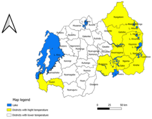
Rwanda is a small landlocked nation located in the Great Lakes region of East Africa. It is at \(02^{0}.00\) latitude south and \(30^{0}.00\) longitude East. It borders Burundi (South), Tanzania (East), Uganda (North) and the Democratic Republic of Congo (DRC) (West). Rwanda has a mild and tropical climate, with temperatures varying across the year, with two maxima and two minima [25]. The average temperature is about 200C, and the topography varies. The warmest temperature is found in the eastern plateau and the south-eastern Rusizi Valley (in the western part of the country) between \(20^{0}\)C and \(21^{0}\)C. The cooler temperatures are found in higher elevations of the central plateau between \(17.5^{0}\)C and \(19^{0}\)C and highlands \((< 17^{0}\)C) in the North of the country. Warner et al., [26] presented in their report the areas in Rwanda mostly facing the risks of droughts. Areas in Rwanda are particularly vulnerable to the devastating impacts of droughts, which have become increasingly frequent and severe in recent years. Climate change is exacerbating this problem, as rising temperatures and changing rainfall patterns are disrupting agricultural productivity, causing water scarcity, and increasing the risk of wildfires. Urgent action is needed to address this pressing issue and develop effective strategies to mitigate the impacts of droughts and promote sustainable development in the affected regions, see Figure 1.

Rwanda experiences two rainy seasons and two dry seasons the year. Rwanda National Meteorological Service announced that the minimum temperature has risen by \(2^{0}\)C over the last 30 years Warner et al., [26]. Therefore, the year 2005 was indicated as the hottest year, with a minimum temperature of \(20.4^{0}\)C and a maximum temperature of \(35^{0}\)C.

5.2. Data description

The daily temperature data was recorded from 9 weather stations collected by the Rwanda Meteorological Agency (RMA) between 2000 and 2017. Those stations are randomly distributed with different temperature patterns and geographical locations due to the area of Rwanda. We analysed the data station by station; the ones with shorter records or high missing data were left out. Unlike statistical analyses regarding climate studies in Rwanda that have used the mean temperature as one of the main variables, this study used extreme value analysis to model the statistical behaviour of extreme temperature. Therefore, annual extreme values were extracted from the daily temperature data from 9 stations and new data set was formed. Under this study uses two methods, the block maxima (BM) method and the Peaks Over Threshold (POT), to model and analyse extracted extreme values.

5.3. Block maxima (BM) and generalized extreme value distribution (GEVD)

Using the BM method, a sample is divided into equal time intervals [27,28], and a set of maximum/minimum observations from each interval constitutes a sample of extremes [1, 29]. Given a sequence of independent and identically distributed random variables \(X_{1m}, X_{2m},..., X_{nm}\) from a time interval, the maximum values are defined as \(M_n=max(X_{1m}, X_{2m},...,X_{nm})\) having a joint distribution function F. The distribution of those maximum values is the Generalized Extreme Value (GEV) distribution: \begin{equation}\notag G(x,\mu,\delta,\xi)=\exp\left[ -\left(1+\xi\left(\frac{x-\mu}{\delta}\right) \right)\right]^{\frac{-1}{\xi}}\,, \end{equation} where \(x\) are the extreme values from the blocks, \(\mu\) a location parameter; \(\delta\) a scale parameter; and \(\xi\) a shape parameter. Referring to the value of shape parameter, the Generalized Extreme Value Distribution has three basic forms, each corresponding to a limiting distribution of maximum values from a different class of underlying distributions. If \(\xi>0\), tails decrease as a polynomial, leading to Fréchet distribution. While \(\xi< 0\), tails are finite, leading to Weibul distribution. A special case is the Gumbel distribution when \(\xi\to 0\): \begin{equation}\notag G(\mu,\delta)=\exp\left[ -\exp\left(-\left(\frac{x-\mu}{\delta}\right) \right)\right]\,. \end{equation}

Peak over threshold (POT) and generalized Pareto distribution (GPD)

One of the methods used to analyze the distribution of extreme events is Peak over Threshold (POT), which considers the maximum variables exceeding a predetermined threshold [20]. In this method, a threshold \(u\) is first fixed, and all data above it are considered extremes. Then, those extreme values of a sample over a chosen threshold are studied by modelling their tail behaviours using the conditional distribution of these exceedances. For example, given that the temperature in Rwanda exceeds a high threshold, let us say \(u\), by how much can \(u\) be exceeded? To answer such a question, we need the Excess Distribution, which is approximated to GPD under Peak Over Threshold (POT) framework. For some sufficiently large threshold \(u\), the distribution of the excess values approximates a Generalized Pareto Distribution with a shape parameter; for some sufficiently large threshold \(u\), the distribution of the excess values approximates a Generalized Pareto Distribution with a shape parameter, \(\xi\) and a scale parameter, \(\delta_u\). Let denote the threshold and \(X\) be a random variable with distribution function \(F\). Then, the exceedances distribution function over the threshold \(u\) is given by \begin{equation}\tag{1} F_{u}(x)=\frac{F(u+x)-F(u)}{1-F(u)}\;if\;X>u,X\geq 0\,. \end{equation} By letting \(Y_i=X_{i}-u\), then the distribution of the exceedances \(Y_1,Y_2,Y_3,...,Y_{nu}\) can be approximated by a Generalized Pareto Distribution with a shape parameter, \(\xi\) and a scale parameter, \(\delta_u\) [20] defined as: \begin{equation}\tag{2}\label{eq2} G(x-\mu,\delta_{u},\xi)=1-\left[1+\xi\left(\frac{x-\mu}{\delta_{u}}\right)\right]^{\frac{-1}{\xi}} \,.\end{equation} Depending on the value of shape parameter, the Generalized Pareto Distribution has three basic forms, each corresponding to a limiting distribution of excess values from a different class of underlying distributions. A special case of Eq. (\ref{eq2}) for \(\xi\to 0\) is the exponential distribution: \begin{equation}\tag{3} G(x-\mu,\delta_{u})=1-\exp\left[ -\left(\left(\frac{x-\mu}{\delta_{u}}\right)\right)\right]\,. \end{equation} The other two cases of Eq. (\ref{eq2}) for \(\xi\neq0\) are as follow:

• If \(\xi >0\), tails decrease as a polynomial, leading to Pareto Distribution.
• If \(\xi< 0\), tails are finite, leading to Beta Distribution.

5.4. Return levels estimation

When the best model for the data is found, the interest is to derive the return levels of maximum temperature. It is vital to evaluate return levels, \(X_T\), for example, the T-year return level, which is exceeded once every T years. The return level of an extreme event, defined as the value \(X_T\), is expected to be exceeded on average once every T year (T is called the return period, that is, the period expressed in years by which the annual observation is expected to return). Let \(Y_T\) represent extreme values of a random variable, such that there is a probability T, that \(Y_T\) is exceeded in any given year. The return level related to the return period \(\frac{1}{T}\) is the level that, on average, is expected to be exceeded once every \(\frac{1}{T}\) years. Let \(X_T\) present the level of exceeded temperature on average only once in T years return level \(X_T=1-\frac{1}{T}\) [30]. In this paper, return levels for both GP and GEV models were estimated and compared.

5.4.1. Return levels estimation for generalized Pareto distribution

Once the GPD is selected as a suitable model for exceedances, then the probability of the exceedances of a variable X over a suitable high threshold \(u\) is \(P(X>x/X>u\) Applying properties of conditional probability and let \(P(X>u)=\tau_u\) to get \(P(X>x)=\tau_u P(X>x/X>u)=\tau_u[1-G(x-u,\delta_u,\xi)]\) which leads to \begin{equation}\tag{4}\label{eq4} P(X>x)=\tau_{u}\left[1+\xi\left(\frac{x-\mu}{\delta_u}\right)\right]^{\frac{-1}{\xi}} \,.\end{equation} Therefore, the amount by which an event exceeds the threshold \(u\) in T-year is obtained by defining \(x_T\) in Eq. (\ref{eq4}) by \(P(X>x_T)=\frac{1}{T}\) and then solve for \(x_T\) Hence, the T-year return level is defined by: \(X_T=u+\frac{\delta_u}{\xi}[T\tau_u]^{\xi}-1\), if \(\xi\neq0\) and \(X_T=u+\delta_u\log(T\tau_u)\), if \(\xi=0\) with \(\tau_u,\) \noindent the probability of the occurrence of an exceedance of a high threshold \(u\) .

5.4.2. Return levels estimation for generalised extreme value distribution

The return level for the GEV model with the return period \(\frac{1}{T}\) is given by [4, 31], \begin{equation}\notag X_T= \left\{ \begin{array}{cc} \mu-\frac{\sigma}{\xi}\{1-[-\log(1-T)]^{\xi}\} & \xi\neq0\\ \mu-\delta\log[1-(-\log(1-T))] & \xi=0 \end{array}\right. \end{equation} The level \(X_p\) is expected to be exceeded on average one every \(\frac{1}{T}\) years.

5.5. Parameter estimation

Considering its consistency, efficiency, asymptotic behaviour, this paper used the method of maximum likelihood estimation (MLE) to estimate GP and GEV parameters. Adaptability of the MLE to changes in model structure as compared to other parameter estimation techniques makes it preferable.

5.5.1. Parameter estimation of generalised Pareto distribution

Let \(Y_1,Y_2,Y_3,...,Y_m\) be a sequence of m excesses of a threshold \(u\). The likelihood function from Eq. (\ref{eq2}) is, \begin{equation}\notag L(y_i,\delta_u,\xi)=\Pi_{i=1}^{n}g(y_i,\delta_u,\xi)\;with\;g(y,\delta_u,\xi)=\frac{d}{dy}G(y,\delta_u,\xi)\,. \end{equation} For \(\xi\neq0\) , the log-likelihood of GPD is \begin{equation}\notag l(y_i,\delta_u,\xi)=-m\log\delta_u-\left(1+\frac{1}{\xi}\right)\sum_{i=1}^{m}\log\left(1+\frac{\xi y_i}{\delta_u} \right)\,, \end{equation} and \begin{equation}\notag l(y_i,\delta_u)==-m\log\delta_u-\frac{1}{\delta_u}\sum_{i=1}^{m}(y_i)\,. \end{equation} For \(\xi=0\). The values \(\delta_u\) and \(\xi\) are the estimation parameters which maximize Eq. (\ref{eq2}).

5.5.2. Parameter estimation of generalised extreme value distribution

Let \((Y_1,Y_2,Y_3,...,Y_k)\) be a random sample of the random variable \(Y\) taken from a GEVD. The log-likelihood function for \(\xi\neq0\) of observed random sample \((Y_1,Y_2,Y_3,...,Y_m)\) is given by, \begin{equation}\tag{5} l\left(\mu,\delta,\sfrac{\xi}{X_1},\ldots,X_m\right)=-mlog\delta-\left(1+\frac{1}{\xi}\right)\sum_{i=1}^{m}log\left(1+\xi\left(\frac{X_i-\mu}{\delta}\right)\right)-\sum_{i=1}^{m}\left(1+\xi\left(\frac{X_i-\mu}{\delta}\right)\right)^\frac{-1}{\xi}\,, \end{equation} provided that \(1+\xi\left(\frac{X_i\mu}{\delta}\right)>0,i=1,2,...,m\). However, when \(\xi=0\) the log-likelihood function becomes \begin{equation}\tag{6}\label{eq5} l(\mu,\delta,\xi/X_1,...,X_m)=-m\log\delta-\sum_{i=1}^{m}\exp\left(\frac{-X_i-\mu}{\delta}\right)-\sum_{i=1}^{m}\left(\frac{X_i-\mu}{\delta}\right)\,. \end{equation} The MLE for the unknown parameters \(\mu,\delta,\xi\) were found by maximizing Eq. (\ref{eq5}). Hence, these equations have been solved by numerical or iteratively methods [32].

6. Numerical results and discussion

This section gives statistical results from the analysis. Table 1 below shows the descriptive measures for the annual maximum temperature at various stations. First, the annual maximum temperatures were obtained by extracting the highest value from the daily temperature in a year, then using R software; basic descriptive statistics were defined.

Table 1. Basic descriptive statistics of annual maximum temperature.

N	Station	Min	Mean	Max	Standard deviation	Shapiro-Wilk Test
1	Kigali	30.9	32.43	33.4	2.079	0.92 (0.013)
2	Rwamagana	30.2	32.08	33.4	2.013	0.91 (0.09)
3	Huye	26.7	30.08	32.3	1.978	0.88 (0.036)
4	Ruhango	30.1	32.29	36.2	2.14	0.90 (0.018)
5	Kibungo	30.2	32.11	34.4	2.066	0.91 (0.11)
6	Nyamata	30.1	32	33.4	2.045	0.87 (0.02)
7	Rusumo	30.2	32.31	33.4	2.363	0.88 (0.03)
8	Ngoma	30.6	32.73	36.5	2.291	0.86 (0.01)
9	Kirehe	29.9	32.26	33.4	2.341	0.91 (0.98)

Table 1 shows how the annual maximum average temperatures have varied throughout each station's considered period. The p-value of the Shapiro-Wilk Test of normality for the annual maxima temperature fails to reject the null hypothesis of a normal distribution for Rwamagana, Kirehe and Kibungo stations. In order words, the null hypothesis for this test is that Rwamagana, Kirehe and Kibungo stations data are normally distributed. Thus, annual maxima are appropriate for extreme value analysis for Kigali, Ngoma, Rusumo, Nyamata, Ruhango, and Huye stations. Furthermore, the stationarity test was done using the Augmented Dickey-Fuller (ADF). Therefore, the null hypothesis that data is nonstationary (has a unit root) is tested in this test. Table 2 presents the stationarity test for maxima temperature.

Table 2. Unit root augmented Dickey-Fuller test for maxima temperature.

Station	Test Statistics	P-value	Conclusion
Kigali	-0.53	0.047	Reject null hypothesis
Huye	-3.82	0.034	Reject null hypothesis
Ruhango	-2.91	0.022	Reject null hypothesis
Nyamata	-4.2	0.016	Reject null hypothesis
Rusumo	-3.66	0.045	Reject null hypothesis
Ngoma	-0.39	0.02	Reject null hypothesis

Based on Table 2, the null hypothesis of nonstationary was rejected for temperature data for all the selected regions (all p-values are less than 5% level of significance).

6.1. The block maxima (BM) method

For GEV estimation, the block maxima of daily annual maximum rainfall are extracted for six stations. Daily temperature observations \(X_{1m},X_{2m},...,X_{nm}\) were divided into equal time intervals (m=12 months) and set of maximum observations from each interval constitutes a sample of extremes called “Annual maxima”. The annual maxima \(M_n=max(X_{1m},X_{2m},...,X_{nm})\) were selected. Annual maxima selected from daily temperature is shown in Figure 2.

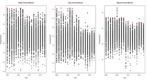
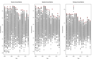
The annual maxima values (in red) selected were fitted to a Generalized Extreme Value (GEV) distribution: \begin{equation}\notag G(x,\mu,\delta,\xi)=\exp\left[-\left( 1+\xi\left(\frac{x-\mu}{\delta}\right)\right)^{\frac{-1}{\xi}}\right]\,, \end{equation} and the location parameter,\(\mu\) ; scale parameter, \(\delta\); and shape parameter, \(\xi\) ; were estimated using method of maximum likelihood estimates (MLE). Table 3 presents the parameter estimates and their corresponding standard errors together with associated confidence interval.

Table 3. GEV parameter estimate for temperature.

Station	Parameter	Estimates	S.E	C.I
Kigali	Location (\(\mu\))	32.439	0.028	(32.321, 32.518)
	Scale (\(\delta\))	1.074	0.019	(0.877, 1.271)
	Shape (\(\xi\))	-1.115	0.006	(-1.312, -0.918)
Huye	Location (\(\mu\))	30.116	2.10-08	(30.110, 30.118)
	Scale (\(\delta\))	2.438	2.10-08	(2.428, 2.448)
	Shape (\(\xi\))	-1.116	2.10-08	(-1.115, -1.118)
Ruhango	Location (\(\mu\))	31.624	0.337	(30.963, 32.285)
	Scale (\(\delta\))	1.234	0.25	(0.744, 1.725)
	Shape (\(\xi\))	-0.047	0.207	(-0.453, 0.359)
Nyamata	Location (\(\mu\))	32.186	0.28	(31.156, 32.346)
	Scale (\(\delta\))	1.347	0.098	(0.978, 1.750)
	Shape (\(\xi\))	-1.11	0.129	(-1.305, -0.978)
Rusumo	Location (\(\mu\))	32.337	0.421	(30.476, 33.002)
	Scale (\(\delta\))	1.064	0.27	(0.997, 1.232)
	Shape (\(\xi\))	-1.001	0.181	(-1.254, -0.789)
Ngoma	Location (\(\mu\))	32.184	0.284	(31.627, 32.742)
	Scale (\(\delta\))	1.09	0.198	(0.702, 1.479)
	Shape (\(\xi\))	-0.072	0.142	(-0.350, 0.205)

The shape parameter (\(\xi\)) is negative for Rusumo, Nyamata, Huye, and Kigali stations. This suggests that the underlying distribution belongs to the Weibul family of distribution. In addition, the confidence intervals of the shape parameter contain zero (0) for Ruhango and Ngoma stations; hence, the Gumbel distribution could be a more accurate model in the entire GEV family. Since Gumbel is one of the GEV models, we used the likelihood ratio test to verify its appropriateness. The estimated parameters for Gumbel model are given in Table 4 while results of likelihood ratio test are given in Table 5.

Table 4. Estimated parameters for Gumbel model.

Station	Parameter	Estimates	S.E	C.I
Pruhango	Location (\(\mu\))	31.593	0.301	(31.002, 32.184)
	Scale (\(\delta\))	1.212	0.225	(0.769, 1.654)
Ngoma	Location (\(\mu\))	32.141	0.225	(31.617, 32.664)
	Scale (\(\delta\))	1.073	0.191	(0.696, 1.449)

Table 5. Likelihood ratio test.

Station	Model	Likelihood-ratio	Chi-square	P-value
Ruhango	M0= Gumbel	0.219	3.841	0.639
	M1=GEV
Ngoma	M0= Gumbel	0.047	3.841	0.827
	M1=GEV

Since GEV and Gumbel are the nested models, we selected the best model on basis of likelihood ration test which is described below: Null hypothesis \(\xi=0\) while alternative hypothesis \(\xi\neq0\). The likelihood ration test results show that Gumbel distribution is the best fit for Ruhango and Ngoma stations.

Graphical model checking

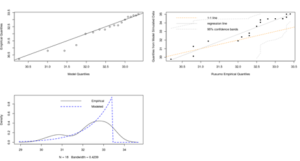
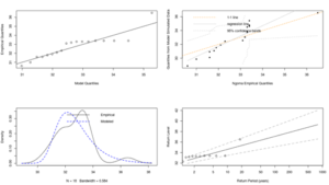
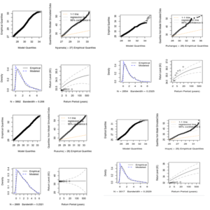
Figures below are the diagnostic plots of the fitted GEV and Gumbel model for the maximum temperature

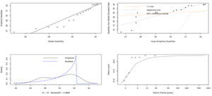
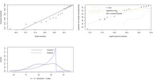
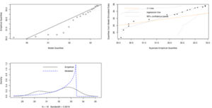
From Figure 3-6 above, the Q-Q and PP plots are not approximately linear as the deviations from the model is very big from the confidence intervals observed on the return level plot for Rusumo, Kigali, Huye and Nyamata stations. Thus, the goodness-of-fit is not satisfied and therefore the fitted GEV distribution seems to be not appropriate.

From Figures 7 and 8 above, the Q-Q and PP plots is approximately linear as the deviations from the model is very small from the confidence intervals observed on the return level plot for Ruhango and Ngoma stations. Thus, the goodness-of-fit is satisfied and therefore the fitted Gumbel distribution is appropriate.

6.2. The peaks over threshold (POT) method

Under the peak-over threshold method, the daily temperature is considered extreme if it exceeds a high threshold \(u\). The excesses over the threshold are approximately distributed by following the Generalized Pareto (GP) distribution. In this study, a generalized Pareto model was fitted to the values exceeding a high threshold and model parameters were estimated using the method of maximum likelihood estimates (MLE). The mean residual life plot and threshold stability were used to choose an appropriate threshold.

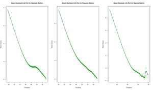
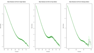
Based on Figure 9, we conclude that the best choice of threshold is approximately \(u=28^oC\) for Kigali, \(u=25^oC\) for Huye, \(u=28^oC\) for Ruhango, \(u=27^oC\) for Nyamata, \(u=28^oC\) for Rusumo, and \(u=27^oC\) for Ngoma for the assumptions of the extreme value approach to be valid. See Table 6 for the GPD parameter estimate for temperature.

Table 6. GPD parameter estimate for temperature.

N	Station	Threshold	Parameter	Estimates	SE	CI
1	Kigali	28	Scale (\(\delta_u\))	2.104	0.049	(1.998, 2.209)
			Shape (\(\xi\))	-0.329	0.012	(-0.364, -0.293)
2	Huye	25	Scale (\(\delta_u\))	4.98	0.047	(1.718, 1.903)
			Shape (\(\xi\))	-0.115	0.018	(-0.152, -0.079)
3	Ruhango	28	Scale (\(\delta_u\))	1.926	0.041	(1.845, 2.007)
			Shape (\(\xi\))	-0.216	0.011	(-0.237, -0.194)
4	Nyamata	27	Scale (\(\delta_u\))	2.139	0.046	(2.049, 2.229)
			Shape (\(\xi\))	-0.253	0.014	(-0.282, -0.233)
5	Rusumo	28	Scale (\(\delta_u\))	2.521	0.057	(2.407, 2.634)
			Shape (\(\xi\))	-0.450	0.015	(-0.479 -0.420)
6	Ngoma	27	Scale (\(\delta_u\))	2.614	0.037	(2.541, 2.686)
			Shape (\(\xi\))	-0.271	0.004	(-0.279, -0.263)

The shape parameter (\(\xi\)) is negative for all six stations. This suggests that the underlying distribution belongs to the Beta family of distribution. In addition, all confidence intervals of the shape parameter do not contain zero (0).

Graphical model checking

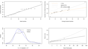
Figures below are the diagnostic plots of the fitted GP model for the maximum temperature.

From Figures 10, the \(Q\)-\(Q\) and \(PP\) plots are approximately linear as the deviations from the model is very small from the confidence intervals observed on the return level plot for all stations. Thus, the goodness-of-fit is satisfied and therefore the fitted GP distribution is appropriate.

They are comparing return levels estimated by Generalized Extreme Values (GEV) with the results of Generalized Pareto Distribution (GPD) in Table 7. No significant differences exist for all periods (T=10, 20, 30, 40, 50, 100) and for all six stations (Kigali, Huye, Ruhango, Nyamata, Rusumo, Ngoma), the predicted return values and the confidence intervals are very close in both GEV and GPD. Return levels show that in Kigali and Ruhango, the temperature will continue to increase within the time period until the temperature goes beyond the current maximum in Table 1 after 100 years. The temperature is predicted to increase in Ngoma, Huye and Rusumo but will not exceed the current maximum temperature highlighted in Table 1. Nyamata, the return level shows that after 30 years for GEV and 100 years for GPD, the temperature will exceed the current maximum temperature, which is \(33.4^{o}C\) as highlighted in Table 1.

7. Conclusion and recommendation

Temperature plays an essential role in various aspects of human life and the environment, including plant growth, rainfall formation, and atmospheric pressure. This study investigated the extreme temperature behavior using the Generalized Extreme Value distribution (GEV) and Generalized Pareto Distribution (GPD) models. The model fit suggests that the Gumbel and Beta distributions are the most appropriate for the annual maximum daily temperature, indicating the probability of extreme temperature events.

Return level estimates and their confidence intervals for the return periods of 10, 20, 30, 40, 50, and 100 years showed that the temperature is projected to increase significantly and may even surpass current maximum temperatures. This finding is concerning and highlights the urgent need for policymakers to take proactive measures to manage the issue of global warming.

Furthermore, the study demonstrated that the goodness-of-fit is satisfied, and the fitted General Pareto Distribution is appropriate compared to the Generalized Extreme Value Distribution. Policymakers must take appropriate measures to address global warming, such as reducing carbon emissions, promoting renewable energy sources, and enhancing energy efficiency.

The findings of this study can help policymakers to make informed decisions that can prevent the adverse impacts of climate change, such as sea-level rise, extreme weather events, and loss of biodiversity. Therefore, it is essential to take proactive measures to manage the issue of global warming, given the forecasted rise in temperature in the years to come.

Further research can explore the regional variations in temperature trends and investigate the underlying mechanisms driving extreme temperature events. The results of this study can help policymakers to create effective policies that mitigate the impacts of climate change and protect human life and the environment.

Table 7. Return level estimation.

		Under BM Approach		Under POT Approach
Station	Period	Return level	CI	Return level	CI
Kigali	10	33.321	(30.398, 36.245)	33.33	(30.408, 36.252)
	20	33.364	(29.101, 37.610)	33.362	(29.105, 37.619)
	30	33.377	(28.060, 38.680)	33.376	(28.071, 38.682)
	40	33.384	(27.178, 39.578)	33.385	(27.182, 39.587)
	50	33.387	(26.370, 40.390)	33.39	(26.389, 40.392)
	100	33.394	(23.200, 43.601)	33.404	(23.202, 43.605)
Huye	10	32.122	(32.121, 32.123)	32.089	(31.147, 33.032)
	20	32.221	(32.22, 32.223)	32.159	(30.864, 33.454)
	30	32.251	(32.250, 32.252)	32.19	(30.630, 33.750)
	40	32.264	(32.263, 32.265)	32.209	(30.429, 33.989)
	50	32.271	(32.270, 32.272)	32.222	(30.251, 34.194)
	100	32. 287	(32.286, 32.288)	32.255	(29.545, 34.966)
Ruhango	10	34.259	(32.967, 35.551)	35.346	(34.915, 35.777)
	20	35.045	(33.200, 36.890)	35.519	(34.990, 36.049)
	30	35.484	(33.210, 37.759)	35.605	(35.007, 36.203)
	40	35.789	(33.166, 38.413)	35.66	(35.008, 36.311)
	50	36.022	(33.105, 38.940)	35.699	(35.002, 36.396)
	100	36.727	(32.775, 40.679)	35.805	(34.947, 36.663)
Nyamata	10	34.259	(31.926, 41.437)	33.368	(28.263, 38.473)
	20	35.045	(30.535, 42.147)	33.386	(25.355, 41.417)
	30	35.484	(29.325, 43.681)	33.393	(22.925, 43.862)
	40	35.789	(29.143, 44.021)	33.397	(20.763, 46.032)
	50	36.022	(28.782, 45.129)	33.4	(18.782, 48.019)
	100	36.727	(27.940, 46.443)	33.406	(10.409, 56.404)
Rusumo	10	33.288	(24.421, 50.862)	33.389	(14.492, 52.286)
	20	33.345	(23.473, 65.325)	33.394	(14.852, 67.532)
	30	33.364	(22.978, 60.185)	33.396	(13.743, 81.644)
	40	33.373	(22.092, 80.127)	33.397	(28.274, 95.068)
	50	33.378	(21.839, 82.003)	33.398	(41.207, 108.003)
	100	33.389	(20.791, 85.572)	33.398	(101.378, 168.175)
Ngoma	10	34.45	(33.413, 35.486)	36.144	(35.085, 37.203)
	20	35.1	(33.738, 36.462)	36.24	(34.810, 37.669)
	30	35.459	(33.858, 37.061)	36.284	(34.580, 37.987)
	40	35.706	(33.914, 37.498)	36.31	(34.381, 38.240)
	50	35.893	(33.942, 37.845)	36.329	(34.204, 38.454)
	100	36.454	(33.948, 38.959)	36.376	(33.508, 39.245)

Author Contributions:

All authors contributed equally in this paper. All authors read and approved the final version of this paper.

Conflicts of Interest:

The authors declare no conflict of interest.