
With the rising demand for advanced thermal management in compact and microscale systems, there’s been a rising interest in understanding how nanofluids behave especially when influenced by electromagnetic and electrokinetic forces. Nanofluids are essentially regular fluids infused with nanoparticles, and they’ve been shown to transfer heat much more efficiently than traditional fluids [1]. Among various nanoparticles, copper (Cu) stands out for its excellent thermal conductivity and its compatibility with water, making Cu–H\(_2\)O nanofluids particularly attractive for use in thermal control applications [2]. Xuan and Li [3] constructed an experimental setup to study the flow characteristics of the nanofluid in a tube and convective heat transfer, for the turbulent flow, measurements are made of the sample nanofluids’ friction factor and convective heat transfer coefficient, there is a thorough discussion of how variables like the Reynolds number and the volume fraction of suspended nanoparticles affect heat transfer and flow characteristics. In their numerical investigation of MHD laminar boundary layer flow with heat and mass transfer of an electrically conducting water-based nanofluid containing gyrotactic microorganisms along a convectively heated stretching sheet, Khan and Makinde [4] discovered that the dimensionless temperature at the surface rises with an increase in the convective parameter while the dimensionless velocity falls with increasing buoyancy ratios and bioconvection Rayleigh numbers. An electrically conducting water-based nanofluid containing three distinct types of nanoparticles copper (Cu), aluminum oxide (Al\(_2\)O\(_3\)), and titanium dioxide (TiO\(_2\)) passed a convectively heated porous vertical plate with variable suction, Mutuku-Njane and Makinde [5] conducted a numerical analysis of the buoyancy and magnetic effects on this steady two-dimensional boundary layer flow. They discovered that increasing the Casson parameter suppresses the velocity field, while temperature and concentration decrease as the Casson parameter increases, also the heat and mass transfer rates decrease as the unsteadiness parameters and Brownian motion parameter increase. In the presence of intense suction, Ahmad et al. [6] investigate the mixed convection boundary layer flow of a nanofluid across a vertical Riga plate, they include the Grinberg-term for the wall parallel Lorentz force caused by the Riga plate in their model, as well as the Brownian motion and thermophoresis effects caused by the nanofluid. MHD free convection in an inclined wavy enclosure with a Cu–water nanofluid and an isothermal corner heater was mathematically modeled by Sheremet et al. [7], while the remaining walls are adiabatic, their work heats the cavity from the bottom left corner and cools it from the top wavy wall. According to Sheikholeslami and Rokni’s [8] analysis of two-phase nanofluid double diffusion convection in the presence of an induced magnetic field, temperature gradient increases with an increase in suction parameters but decreases with an increase in thermophoretic parameters, and nanofluid motion decreases with an increase in Schmidt and Hartmann numbers but increases with an increase in buoyancy ratio and thermophoretic parameters. Sheikholeslami et al. [9] simulated the magnetohydrodynamic (MHD) forced convective heat transfer inside a porous three-dimensional enclosure with a heated cubic obstacle using the Lattice Boltzmann Method (LBM). Al\(_2\)O\(_3\)-H\(_2\)O nanofluid has been used using a singlephase model in mind. Their analysis demonstrates that when the Reynolds and Darcy numbers increase, the temperature boundary layer gets thinner. Using the non-homogeneous model for nanofluids, Pal et al. [10] performed a computational analysis of conjugate heat transfer resulting from the combined convection and conduction of a Cu-water nanofluid in a thick-wall enclosure. They consider an enclosure with a thick wavy heated left side wall with the right vertical wall being permitted to travel vertically downwards to generate a shear driven flow. This causes mixed convection inside the enclosure when combined with the horizontal temperature gradient. In a vertical channel filled with nanofluid and an induced magnetic field, Jha and Samaila [11] investigated the effect of heat source/sink on magnetohydrodynamics free convection flow. According to their findings, the shear stress is increased by the Brownian motion parameter (Nb) and buoyancy ratio (Br), whereas the thermophoretic parameter (Nt) and Hartman number (Ha) show the opposite effect. Additionally, it shows that the induced current density is increased by the Hartman number (Ha) and thermophoretic parameter (Nt), whereas the opposite is true for the heat sink parameter (-S). Mng’ang’a [12] has studied the effects of Newtonian heating, induced magnetic field, and Ohmic heating on the generalized Couette flow of Jeffrey nanofluid in MHD between two horizontal plates with convective cooling. According to his research, concentration profiles drop as the Schmidt number rises, while velocity profiles decrease as the Jeffrey parameter rises. Additionally, it reveals that Cu-water has a considerable effect on temperature and velocity in the generalized Couette channel compared to nanofluid. The study of the Joule and viscous dissipation effects for improving nuclear reactor and automobile radiator coolants in mechanical systems has received a lot of attention. Oni et al. [13] used Tiwari-Das to include the effects of nanoparticles in the deterministic model. Their model offers a thorough foundation for comprehending how the behavior of the system is influenced by the presence of nanoparticles. Therefore, for Al\(_3\)O\(_3\) and Cu nanoparticles, the model includes the dynamics of Joule heating, electric current density, Darcy, and viscous dissipation in the energy conservation equation.
Due to its applications in a variety of engineering and industrial processes, including magnetic drug targeting, electronic device cooling, and energy systems, the study of magnetohydrodynamic (MHD) flows has attracted a lot of attention. Magnetohydrodynamic (MHD) flow is the flow that is propelled by the Lorentz force due to the interaction of electric currents with a vertical magnetic field. In particular, the impact of magnetic fields on electrically conducting fluids, such as nanofluids, has been thoroughly investigated to improve heat and mass transfer characteristics [14, 15]. In systems where the magnetic Reynolds number is non-negligible, the induced magnetic field produced by the motion of the conducting fluid itself is essential, even though many studies solely take into account an externally supplied magnetic field. If this induced component is ignored, the actual fluid behavior and related thermal transport processes may not be accurately predicted. [16, 17]. As one of the most important areas of fluid dynamics, MHD piques the attention of several researchers, who study the effects of electric and magnetic forces on the flow of electrically conducting fluids [18]. Chamkha [19] looked into the problem of free convection flow of an electrically conducting fluid up a vertical plate embedded in a thermally stratified porous media under the influence of a uniform normal magnetic field. Jha [20] examined the combined effects of free convection and a uniform transverse magnetic field on the couette flow of an electrically conducting fluid between two parallel plates for impulsive motion of one of the plates, assuming that the applied magnetic field and the negligible induced magnetic field were fixed with respect to the fluid or tube. Moghaddam [21] analyzed the performance of MHD micropumps numerically assuming that the viscosity of the fluid is shear-dependent, he discovered that shear-thinning fluids produce a greater flow rate as compared to Newtonian fluids provided that the Hartmann number is above a certain point. Under the influence of a vertical magnetic field. Jian [22] analytical studies the coupled unsteady electroosmotic, pressure-driven, and magnetohydrodynamic (MHD) flow of an electrically conducting, incompressible, and viscous fluid through a slit parallel plate microchannel. In a vertical annular micro-channel made up of two concentric cylinders, Jha and Aina [23] examine the impact of an induced magnetic field on the fully developed magnetohydrodynamic (MHD) natural convection flow of an electrically conducting fluid in the presence of an imposed radial magnetic field. They consider the temperature jump and velocity slip at the annular micro-channel surfaces, as well as the influence of an induced magnetic field resulting from the motion of an emotionally charged fluid. Yang et al. [24] theoretically investigate the heat transfer properties of incomprehensible magnetohydrodynamic electroosmotic flow through a two-dimensional rectangular microchannel. They apply a lateral electric field and a vertical magnetic field to an existing axial electric field in order to take into account the electromagnetic effect under the combined electrokinetic effect. Jha and Gwandu [25] examined a free convective flow of an electrically conducting fluid and an incompressible MHD through a vertical micro-channel with a rectangular shape; both plates were porous and heated alternately. The study examined the effects of super-hydrophobicity, magnetism, and wall porosity on the flow’s fundamental characteristics. In the presence of a transverse magnetic field, Jha et al. [26] examined the run-up flow of an incompressible, viscous, Newtonian fluid in magnetohydrodynamics (MHD) that is surrounded by two parallel horizontal porous plates. They found that the disturbances coming from the border into the fluid are what cause the momentum to be transferred. Taking into consideration the effects of magnetic induction, ion slip, and Hall current, Jha and Malgwi [27] examined the interaction of conducting and nonconductive walls on transient MHD buoyancy driven flow of Newtonian fluid in a permeable microchannel. Their findings indicate that when the appropriate micro-porous wall is electrically conducting and introduces the effects of ion slip current, they noticed that Hall current helps to strengthen secondary generated magnetic field while diminishing it in other cases. Muhammad et al. [28] examine how inverse-square heat absorption affects steady, fully developed laminar MHD natural convection flow in an infinite vertical concentric annulus while applying radial and induced magnetic fields. They find that while stronger magnetic fields suppress fluid motion, lowering mass flux and increasing flow resistance, increasing the heat absorption parameter intensifies thermal gradients close to the inner cylinder. Mandadi and Mella [29] examine how the magnetohydrodynamic (MHD) boundary layer flow of a Williamson nano fluid over a permeable stretched sheet with slip effects is affected by viscous dissipation, heat source, and chemical reaction. Using an induced magnetic field (IMF) and a relatively high concentration of foreign mass (to account for Soret and Dufour effects), Paddar et al. [30] numerically analyze the steadystate solution for transient magnetohydrodynamic (MHD) dissipative and radiative fluid flow over a vertically oriented semi-infinite plate.
On the other hand, electromagnetohydrodynamics (EMHD) expands on Magnetohydrodynamics (MHD) by taking into account both electric and magnetic field effects at the same time. MHD studies the dynamics of electrically conducting fluids under the influence of magnetic fields, which is essential for applications ranging from plasma confinement to metallurgical processes [31] and [32]. Particularly in microscale and nanoscale systems where electrokinetic forces are important, EMHD focuses on situations in which electric fields have an equally prominent role. Since its inception in the field of plasma physics [33], EMHD has gained increasing attention in the fields of microfluidic and biomedical engineering, where accurate fluid flow control is crucial [34]. Richer and more complicated flow patterns are produced by EMHD, which combines electroosmotic, electrophoretic, and Lorentz force effects, in contrast to classical MHD, which primarily includes Lorentz forces originating from current–magnetic field interactions [35]. In electroosmotic-driven microchannel flows, which are frequently found in lab-on-a-chip technologies, where the electric double layer (EDL) dynamics significantly affect flow properties, this dual-field interaction has a particularly significant impact [36]. Recent research has demonstrated the potential of EMHD in improving heat and mass transfer, particularly in small systems where passive approaches are inadequate [37]. For example, incorporating EMHD principles into thermal management systems enables non-mechanical pumping, lower power consumption, and better control over flow and temperature profiles [38]. Additionally, EMHDdriven flows have demonstrated potential in applications like targeted drug delivery, biomolecular manipulation, and microscale cooling of high-performance electronics [39]. Analysis of electromagnetohydrodynamic (EMHD) fluxes in complicated fluids has advanced significantly through the use of perturbation techniques. For example, Si and Jian [40] used the perturbation approach to get approximate analytical solutions for the volume flow rate and velocity of an electrically conducting, incompressible, and viscous Jeffrey fluid between two slit microparallel plates with walls that are sinusoidally corrugated. A developed electron magnetohydrodynamics (EMHD) soliton model was proposed by Li et al. [41] as a novel approach to the formation of small-scale magnetic holes (SSMHs) in the magnetosphere plasma sheet. The Biermann battery effect is taken into consideration when resolving the magnetic evolution equation with a slowmode solution in the weak nonlinear regime. Mandula et al. [42] used a perturbation method to analyze EMHD flow in microchannels with sinusoidally corrugated walls, looking at both in-phase and out-of-phase configurations. The numerical results showed that walls phase differences become insignificant at higher wavenumbers, and that corrugation effects decrease with increasing Hartmann number. It’s interesting to note that, below a threshold wavenumber, out-of-phase corrugations can increase mean velocity, while in-phase corrugations consistently decrease flow. Jian and Chang [43] used Gauss integration and the modification of parameters approach to offer an analytical solution for EMHD flow in a slit microchannel with a non-uniform vertical magnetic field and a lateral electric field. Excellent agreement with numerical results was demonstrated by validation using Chebyshev spectral collocation. With comparisons to experimental data, the study visually examined how velocity profiles were affected by Hartmann number, electric field strength, and magnetic field decay. Rashid et al. [44] studied EMHD flow of a second-grade fluid through a porous medium between microparallel plates with sinusoidally corrugated walls, in both in-phase and out-of-phase configurations. Analytical solutions for velocity and flow rate were found using perturbation techniques, demonstrating the influence of variables such as amplitude ratio on velocity. Interestingly, wave impacts on flow behavior are minimized at lower amplitude ratios. Using lubrication theory and finite volume methods, Mondal et al. [45] conducted a theoretical analysis of electromagnetic heat transfer (EMHD) flow in vertical hydrophobic microchannels, taking into account temperature-dependent viscosity, electrical, and thermal conductivities. The study looked at entropy generation (as measured by the Bejan number), slip effects, and electromagnetic transport, emphasizing how thermophysical variations affect temperature distribution and electroosmotic flow, with validations against experimental data. Bhatti et al. [46] used a modified Darcy–Brinkman–Forchheimer model to account for the effects of porous media and a transverse magnetic field and axial electrical field to develop a mathematical model for laminar, steady state fully developed viscoelastic natural convection electromagnetohydrodynamic (EMHD) flow in a microchannel with a porous medium. The effects of EMHD electroosmotic flow of a hybrid nanofluid through circular cylindrical microchannels are investigated by Bilal et al. [47]. They analyze a hybrid nanofluid that contains four distinct nanomaterials: copper, silver, and single and multiwall carbon nanotubes. They used the Yamada– Ota model for the single and multiwall carbon nanotubes, while the Xue model is used for the copper and silver hybrid nanofluid to specify the thermal conductivity. For the steady, laminar EMHD flow of a flammable non-Newtonian Carreau fluid in a porous vertical duct under coupled electric and magnetic fields, Bhatti et al. [48] created a mathematical model. Suction/injection at permeable walls, viscous and Joule heating, and Forchheimer effects are all included in the study. The Adomian decomposition method was used to validate the results after Frank-Kamenetskii theory and a shooting method were applied. Using thermal/solute stratification and non-Fourier heat flux, Gupta et al. [49] examined the 3D laminar EMHD flow of a Maxwell nanofluid (engine oil containing cobalt ferrite nanoparticles) across an exponentially extending surface. They examined velocity, temperature, and concentration profiles using the Optimal Homotopy Analysis Method, emphasizing the impact of important dimensionless parameters and providing thorough comparisons to the body of previous work.
Recently, flows influenced by electromagnetohydrodynamics (EMHD) have gained attention, especially for technologies like lab-on-a-chip devices, biomedical tools, and microelectromechanical systems (MEMS) [50]. In these systems, fluid motion is mainly driven by electromagnetic forces. Adding electroosmotic effects into the mix allows for even better flow control without relying on mechanical pumps a big advantage when precision and efficiency matter [51]. When you also consider Jeffery fluid models, which represent non-Newtonian fluids with suspended ellipsoidal particles, the picture becomes even more realistic and complex [52]. Pikal [53] addressed the principles of electroosmotic flow in transdermal iontophoresis, noting its crucial role in increasing drug transport, especially for large ions, and outlining how electroosmosis promotes anodic delivery while inhibiting cathodic delivery. The effects of the electrical doublelayer and applied fields on velocity, pressure drop, and skin friction were demonstrated by Yang et al. [54] through numerical analysis of electroosmotic flow in microchannels with a 90° bend. At higher Reynolds numbers, there were noticeable changes in pressure and flow separation. Dutta et al. [55] employed a spectral element method to simulate pure and coupled electroosmotic/pressure6 driven Stokes flows in cross-flow and Y-split junctions, showing linear flow control via electric fields and effective resolution of thin double layers for complex geometries. Kang et al. [56] analytically explored dynamic electroosmotic flow in cylindrical capillaries using the entire Poisson–Boltzmann equation and Green’s function approach, focusing on transient responses to AC electric fields and studying frequency-dependent effects and limiting cases. Ghosal [57] went over the basic principles of electroosmotic flow (EOF) in capillary electrophoresis, emphasizing how it might improve microfluidic transport while also possibly decreasing separation efficiency in the event of flow distortions. With a focus on how temperature-induced changes affect fluid mechanics, heat/mass transfer, and overall microfluidic device performance, Xuan [58] reviewed recent developments on Joule heating effects in electroosmotic flow. Using electroosmosis, electrophoresis, and streaming potentials, Zhao and Yang [59] gave a thorough overview of electrokinetic phenomena in non-Newtonian fluids. They highlighted how the coupling of non- Newtonian hydrodynamics and electrostatics complicates flow behavior, pointing out that shearthinning fluids increase electrokinetic effects while shear-thickening fluids decrease them. They also listed important theoretical issues and future research directions. In nanofluidic channels with different depths, Haywood et al. [60] evaluated electroosmotic mobilities. They compared the results with Poisson-Boltzmann theory, demonstrating significant confinement effects with decreased mobility at low \(\kappa h\) and strong agreement at high \(\kappa h\). Through the use of Navier’s slip law and s-PTT rheology, Sarma et al. [61] modeled the electroosmotic flow of a viscoelastic fluid in a parallel-plate microchannel with high zeta potential. Analytical solutions for potential, velocity, and flow rate (without the Debye-Hückel approximation) showed that slip, zeta potential, and viscoelasticity all work together to improve flow, providing important information for the design of microfluidic systems. Four non-Newtonian polymer solutions’ electroosmotic flow via a constriction microchannel under DC electric fields was experimentally examined by Ko et al. [62]. They discovered that XG displayed elevated center jets and flow vortices as a result of shearthinning, whereas weakly shear-thinning PVP and PEO behaved similarly to Newtonian fluids. These vortices were repressed by very viscoelastic PAA, demonstrating clear rheological impacts on flow dynamics. Using Joule heating, chemical reactions, and viscous dissipation, Nadeem et al. [63] examined microvascular blood flow with heat and mass transfer in a wavy microchannel controlled by electroosmosis. They obtained analytical solutions to investigate temperature, concentration, and pressure rise using Debye-Hückel and lubrication theory, offering comprehensive insights into flow and pumping characteristics. Luo and Keh [64] solved the Poisson-Boltzmann and modified Navier-Stokes equations to study the electric conduction and electroosmotic flow of a salt-free solution in a charged circular capillary. Their conclusions, which were in good agreement with actual data, were based on closed-form formulas that demonstrated the effects of surface charge density and electrokinetic radius on mobility and conductivity. As fluid systems move from the micro- to nanoscale, Alizadeh et al. [65] reviewed the foundations and evolution of electrical double layer (EDL) models in electroosmotic flow, outlining significant theoretical and experimental developments. By taking into account slip boundary conditions and asymmetric wall potentials, Wang et al. [66] investigated unsteady electroosmotic flow of viscoelastic fluids in a parallel plate microchannel with a magnetic field. They obtained both analytical and numerical solutions, demonstrating excellent agreement and examining the effects of different parameters on velocity profiles. Oni and Rilwan [67] examined time-dependent EMHD natural convection flow with electroosmotic effects in a vertical microchannel under suction/injection influence. Using Laplace transforms and Riemann sum approximation, they derived semi-analytical solutions for velocity and temperature, validated by MATLAB simulations. Their findings include specifics on the effects of suction/injection and variables such as the Grashof number, Hartmann number, electric field strength, and Prandtl number on flow dynamics. In order to determine precise solutions for velocity, temperature, and potential using undetermined coefficients and Debye–Hückel linearization, Rilwan et al. [68] investigated the effects of Joule heating, viscous dissipation, and EDL effects on steady Electroosmotic EMHD flow in a porous microchannel. Their MATLAB simulations demonstrate how parameters such as Brinkmann number, Joule heating, Hartmann number, and suction/injection shape flow and heat transfer. Rilwan et al. [69] used Debye–Hückel linearization and undetermined coefficients to analyze steady Electroosmotic EMHD flow in a microchannel and derive exact solutions for electric potential, velocity, and temperature profiles under Joule heating, viscous dissipation, and EOF effects. Their results show how parameters such as Brinkmann number, Hartmann number, and electric field strength have a significant impact on flow and heat transfer.
Although plenty of research has been done on nanofluids and EMHD effects separately, there’s still a gap when it comes to studying all these aspects together particularly for Jeffery nanofluids under the combined influence of electroosmosis and EMHD. The novelty of this study lies in investigating the combined effects of induced magnetic field, slip boundary condition, and natural convection on electromagnetic hydrodynamic (EMHD) and electroosmotic (EOF) flow of Jeffrey nanofluids between two vertical plates. The model incorporates the influence of an applied magnetic field and electrokinetic effects, providing a comprehensive description of the coupled transport mechanisms. The nanofluid used consists of pure water as the base fluid with copper (Cu) nanoparticles, known for their excellent thermal conductivity and heat transfer enhancement. To the best of the authors’ knowledge, the simultaneous analysis of EMHD, EOF, slip boundary effects, and natural convection in Jeffrey nanofluid flows between vertical plates has not been extensively reported in the literature. These kinds of flows are crucial in a variety of engineering and technological applications, including microfluidic devices, electronic cooling systems, heat exchangers, biomedical transport systems, nanofluid-based solar collectors, and electroosmotic pumps.
A microchannel heat exchanger for electronic cooling. A copper-water nanofluid flows through extremely small channels in this instance, and magnetic fields regulate the flow to enhance heat removal. This arrangement is used in high-power electronics and computer chips to efficiently dissipate heat.
A biomedical microfluidic drug delivery device is used in targeted drug delivery, lab-on-a-chip diagnostics, and controlled therapeutic applications. It guides drug-loaded nanoparticles through tiny capillaries or microchannels using magnetic and electroosmotic forces. For improved heat transfer or drug transport performance, the induced magnetic fields, electroosmotic effects, and slip conditions all work together to control and optimize the flow behavior. The governing system of nonlinear partial differential equations (PDEs) is formulated and solved using the finite difference method for the transient state and undetermined coefficient for the steady state, with numerical implementation in MATLAB, enabling a detailed parametric investigation of the flow and thermal fields.

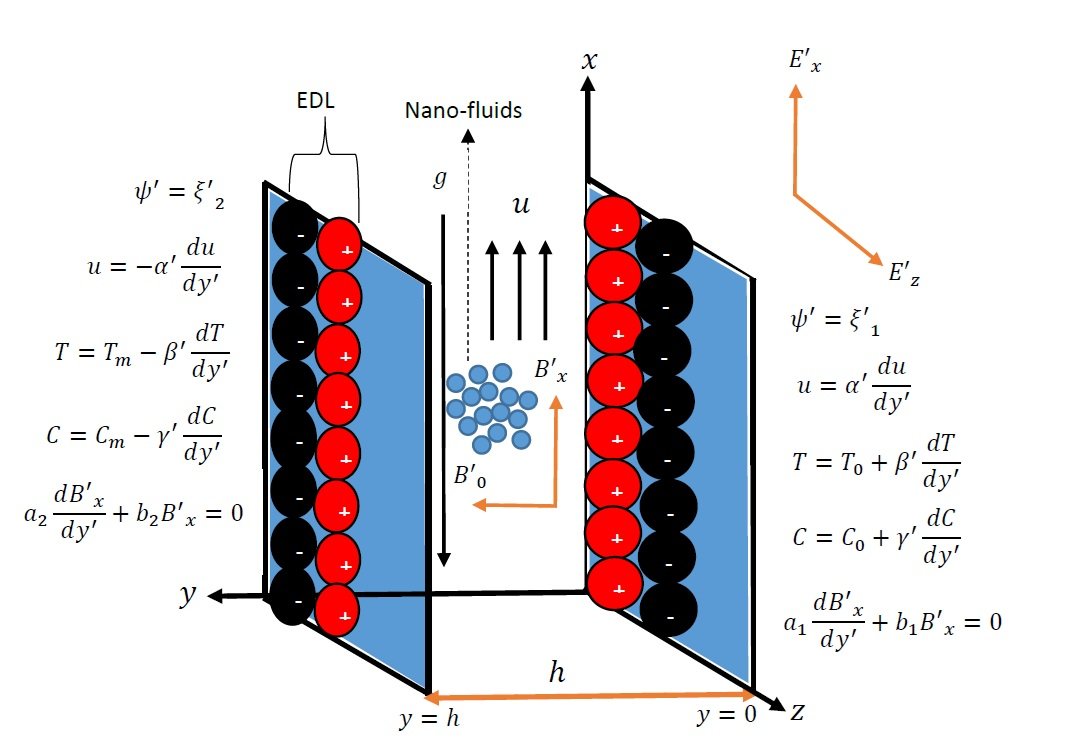
Consider a transient, laminar, electromagnetohydrodynamic free convection flow in a fully developed region of incompressible, viscous and electrically conducting fluid of Jeffery nanofluid, in vertical plates with electroosmotic effects in the presence of transversely applied magnetic field with induced magnetic effect. The \(x-\)axis is parallel to the flow direction of the fluid while \(y-\)axis is perpendicular to the flow direction as illustrated in Figure 2. The width \(h\) separating the plates is minimal when compare with length of the plates. The flow velocity \(u\) and the magnetic field vectors are respectively given as \(\vec{U}=(u,0,0)\) and \(\vec{B}=(B'_x,B'_0,0)\). Using Mng’Ang’A [12] together with Jha and Oni [70] the governing equations of EMHD with induced magnetic field and EOF of Jeffery fluid are obtained based on the following assumptions:
It is assumed that electroosmotic flow and a constant pressure gradient drive the flow;
The flow direction is perpendicular to a uniform magnetic field strength \(B'_0\);
Ion convection effects are minimal since the charge distribution in the EDL is consistent with the Boltzmann distribution;
Debye–Hückel linearization is assumed because the wall potentials are sufficiently low;
All thermophysical and hydrodynamic parameters are taken to be constant unless otherwise noted.
With the assumptions and mathematical expression of Poisson–Boltzmann equation from Chapman [71] and Gouy [72], they state that the EDL potential distribution \(\psi'\) with a constant permittivity (\(\varepsilon\)) as a function of a uniform charge density (\(\rho_e\)) may be defined using the Poisson equation as follows: \[\label{eq1} \nabla^2 \psi' = -\frac{\rho_e}{\varepsilon} , \tag{1}\] where \(\rho_e\) can be expressed as \(\rho_e = e(w_+ n_+ – w_- n_-)\) and \(n_{\pm} = n_0 \exp \left( \frac{w_{\pm} e \psi'}{K_B T} \right)\).
Here, \(T\) is the temperature on an absolute scale, \(K_B\) is the Boltzmann constant, \(n_0\) is the bulk ionic concentration, \(\varepsilon\) is the electrons’ ionic-charge density, \(w_{\pm}\) is valency, and \(n_{\pm}\) is the positively and negatively charged species’ ionic number density.
The Debye–Hückel linearization approximation is used to approximate Eq. (1), turning it into a linear equation in Cartesian as follows: \[\label{eq2} \frac{d^2 \psi'}{dy^2} = \kappa^2 \psi', \tag{2}\] subject to: \[\label{eq3} \psi'(0) = \xi'_1 \text{ and } \psi'(h) = \xi'_2. \tag{3}\]
The continuity and Navier–Stokes equations for transient and steady state (SS) of the flow formation in the flow field can be respectively expressed as: \[\label{eq4} \nabla \cdot \vec{U} = \frac{\partial u}{\partial x} + \frac{\partial v}{\partial y} + \frac{\partial w}{\partial z} = 0 , \tag{4}\] \[\begin{aligned} \label{eq5} -\nabla p – &\frac{\mu_{nf}}{\rho_{nf} \kappa_p} \vec{U} + \left( \frac{\mu_{nf}}{1 + \lambda} \right) \nabla^2 \vec{U} + \frac{\rho_e \xi'}{\rho_{nf}} (\mu_e)_{nf} (\vec{\nabla} \times \vec{B})\notag\\ & \times \vec{B} + g \beta_T \rho_{nf} (T – T_w) + g \beta_C \rho_{nf} (C – C_w) = 0 \quad \text{(SS)} , \end{aligned} \tag{5}\] \[\begin{aligned} \label{eq6} \rho_{nf} \left( \frac{\partial \vec{U}}{\partial t} + (\vec{U} \cdot \nabla \vec{U}) \right) =& -\nabla p – \frac{\mu_{nf}}{\kappa_p} \vec{U} + \left( \frac{\mu_{nf}}{1+\lambda} \right) \nabla^2 \vec{U} + \rho_e \vec{E} + (\mu_e)_{nf} (\nabla \times \vec{B})\notag\\ & \times \vec{B} + g \beta_T \rho_{nf} (T – T_w) + g \beta_C \rho_{nf} (C – C_w), \text{(Trasient),} \end{aligned} \tag{6}\] subject to: \[\label{eq7} u'(0) = \alpha' \frac{du'(0)}{dy'} \quad \text{and} \quad u'(h) = \alpha' \frac{du'(h)}{dy'}. \tag{7}\]
The EMHD flow field’s energy equations is expressed in dimensional vector form as: \[\label{eq8} \frac{k_{nf}}{(\rho C_p)_{nf}} \nabla^2 T = 0 \quad \text{(SS)}, \tag{8}\] \[\label{eq9} \rho C_p{}_{nf} \left( \frac{\partial T}{\partial t} + (\vec{U} \cdot \nabla T) \right) = k_{nf} \nabla^2 T \quad \text{(Transient)}, \tag{9}\] subject to: \[\label{eq10} T(0) = T_0 + \beta' \frac{dT(0)}{dy'} \quad \text{and} \quad T(h) = T_m – \beta' \frac{dT(h)}{dy'}. \tag{10}\]
The EMHD flow field’s concentration equations is expressed in dimensional vector form as:
\[\label{eq11} D_m \nabla^2 C = 0 \quad \text{(SS)}, \tag{11}\]
\[\label{eq12} \left( \frac{\partial C}{\partial t} + (\vec{U} \cdot \nabla C) \right) = D_m \nabla^2 C \quad \text{(Transient)}, \tag{12}\] subject to: \[\label{eq13} C(0) = C_0 + \gamma' \frac{dC(0)}{dy'} \quad \text{and} \quad C(h) = C_m – \gamma' \frac{dC(h)}{dy'}. \tag{13}\]
The EMHD flow field’s Induced magnetic equations is expressed in dimensional vector form as: \[\label{eq14} \vec{\nabla} \times (\vec{u'} \times \vec{B}) + \frac{1}{(\mu_e)_{nf} \sigma_{nf}} (\nabla^2 \vec{B}) = 0 \quad \text{(SS)}, \tag{14}\]
\[\label{eq15} \frac{\partial \vec{B}}{\partial t} = \vec{\nabla} \times (\vec{u'} \times \vec{B}) + \frac{1}{(\mu_e)_{nf} \sigma_{nf}} (\nabla^2 \vec{B}) \quad \text{(Transient)}, \tag{15}\] subject to: \[\label{eq16} \alpha'_1 \frac{dB'_x(0)}{dy'} + b_1 B'_x(0) = 0 \quad \text{and} \quad \alpha'_2 \frac{dB'_x(h)}{dy'} + b_2 B'_x(h) = 0. \tag{16}\]
The fluid motion, energy, concentration and induction equations are expressed in Cartesian as:
Steady State:
\[\begin{aligned} \label{eq17} -\frac{1}{\rho_{nf}} \frac{dp'}{dx'}& – \frac{\mu_{nf}}{\rho_{nf} \kappa_p} u' + \left( \frac{\nu_{nf}}{1 + \lambda} \right) \frac{d^2 u'}{dy'^2}+ g \beta_T \rho_{nf}(T – T_{\infty})\notag\\ & + g \beta_C \rho_{nf}(C – C_{\infty}) + \frac{\rho_e E'_x}{\rho_{nf}} + (\mu_e)_{nf} \left( B_0 \frac{dB'_x}{dy'} \right) = 0, \end{aligned} \tag{17}\]
\[\label{eq18} \frac{k_{nf}}{(\rho C_p)_{nf}} \left( \frac{d^2 T}{dy'^2} \right) = 0, \tag{18}\]
\[\label{eq19} D_m \frac{d^2 C}{dy'^2} = 0, \tag{19}\]
\[\label{eq20} B_0 \frac{du'}{dy'} + \frac{1}{(\mu_e)_{nf} \sigma_{nf}} \left( \frac{d^2 B'_x}{dy'^2} \right) = 0. \tag{20}\] Transient:
\[\begin{aligned} \label{eq21} \frac{\partial u'}{\partial t} =& -\frac{1}{\rho_{nf}} \frac{\partial p'}{\partial x'} – \frac{\mu_{nf}}{\rho_{nf} \kappa_p} u' + \left( \frac{\nu_{nf}}{1 + \lambda} \right) \frac{\partial^2 u'}{\partial y'^2} + g \beta_T \rho_{nf}(T – T_{\infty})\notag\\ &+ g \beta_C \rho_{nf}(C – C_{\infty}) + \frac{\rho_e E'_x}{\rho_{nf}} + (\mu_e)_{nf} \left( B_0 \frac{\partial B'_x}{\partial y'} \right), \end{aligned} \tag{21}\]
\[\label{eq22} \frac{\partial T}{\partial t} = \frac{k_{nf}}{(\rho C_p)_{nf}} \left( \frac{\partial^2 T}{\partial y'^2} \right), \tag{22}\]
\[\label{eq23} \frac{\partial C}{\partial t} = D_m \frac{\partial^2 C}{\partial y'^2}, \tag{23}\]
\[\label{eq24} \frac{\partial B'_x}{\partial t} = B_0 \frac{\partial u'}{\partial y'} + \frac{1}{(\mu_e)_{nf} \sigma_{nf}} \left( \frac{\partial^2 B'_x}{\partial y'^2} \right). \tag{24}\]
| Property | Water (\(H_2O\)) | Copper (\(Cu\)) |
|---|---|---|
| Density (\(\rho\)) (kg/m\(^3\)) | 997 (at 25\(^\circ\)C) | 8960 |
| Viscosity (\(\nu\)) (Pa·s) | \(0.89 \times 10^{-3}\) | – |
| Specific Heat Capacity (\(C_p\)) (J/kg·K) | 4184 | 385 |
| Coefficient of Thermal Expansion (\(\beta\)) (1/K) | \(6.9 \times 10^{-5}\) | \(1.7 \times 10^{-5}\) |
| Magnetic Permeability (\(\mu_e\)) (H/m or N/A\(^2\)) | \(1.2566 \times 10^{-6}\) | \(1.2566 \times 10^{-6}\) |
| Electrical Conductivity (\(\sigma\)) (S/m) | \(5.5 \times 10^{-6}\) | \(5.96 \times 10^7\) |
| Thermal Conductivity (\(k\)) (W/m·K) | 0.606 | 401 |
The thermophysical properties of pure water as the base fluid and Copper (Cu) as the nanoparticles are considered and values are presented in Table 1, while the Brinkmann-type nanofluid as Mng’Ang’A [12] is given below:
\[\begin{aligned} \label{eq25} \begin{cases} \rho_{nf} = (1 – \phi)\rho_f + \phi \rho_s, \quad \nu_{nf} = \frac{\mu_{nf}}{\rho_{nf}}, \quad \frac{k_{nf}}{k_f} = \frac{k_s + 2k_f – 2\phi(k_f – k_s)}{k_s + 2k_f + \phi(k_f – k_s)}, \quad \mu_{nf} = \frac{\mu_f}{(1 – \phi)^{2.5}}, \\ (\rho C_p)_{nf} = (1 – \phi)(\rho C_p)_f + \phi (\rho C_p)_s, \quad \frac{\sigma_{nf}}{\sigma_f} = 1 + \frac{3(\tau_1 – 1)\phi}{(\tau_1 + 2) – (\tau_1 – 1)\phi}, \quad \tau_1 = \frac{\sigma_s}{\sigma_f}, \quad \alpha_{nf} = \frac{k_{nf}}{(\rho C_p)_{nf}}, \\ (\mu_e)_{nf} = (1 – \phi)\mu_{e_f} + \phi \mu_{e_s}, \quad (\beta_T)_{nf} = (1 – \phi)\beta_{T_f} + \phi \beta_{T_s}, \quad (\beta_C)_{nf} = (1 – \phi)\beta_{C_f} + \phi \beta_{C_s}.\end{cases} \end{aligned} \tag{25}\]
The governing Eqs. (2) and (17) to (24), along with their boundary conditions, are non-dimensionalized by introducing the following non-dimensional variables and parameters:
\[\begin{aligned} \label{eq26} \begin{cases} u = \frac{w}{U}, \quad t = \frac{tU}{h}, \quad y = \frac{y'}{h}, \quad x = \frac{x'}{h}, \quad p = \frac{p h}{\mu_f U}, \quad B_x = \frac{B'_x}{B_0 \sigma_f \mu_{e_{nf}} U}, \quad K = kh, \quad \psi = \frac{\psi'}{\xi}, \\ \xi_1 = \frac{\xi'_1}{\xi}, \quad \xi_2 = \frac{\xi'_2}{\xi}, \quad E_x = \frac{E_x \xi}{h \rho_f U^2}, \quad \rho_e = -\kappa^2 \xi \frac{\psi}{h^2}, \quad Re = \frac{Uh}{\nu_f}, \quad Da = \frac{h^2}{\kappa_p}, \quad Gr = \frac{g \beta_T (T_w – T_\infty) h}{U^2}, \\ G_C = \frac{g \beta_C (T_w – T_\infty) h}{U^2}, \quad Pr = \frac{\mu_f C_p}{k_f}, \quad Sc = \frac{\nu_f}{D_m}, \quad Pr_m = \mu_e \sigma_f \nu_f, \quad \theta = \frac{T – T_0}{T_\infty – T_0}, \quad \phi = \frac{C – C_0}{C_w – C_0}, \\ M^2 = \frac{\sigma_f \mu_e B_0^2 h^2 \nu_f}{\mu_f}, \quad a_1 = \frac{a_1'}{h}, \quad a_2 = \frac{a_2'}{h}, \quad b_1 = \frac{b_1'}{h}, \quad b_2 = \frac{b_2'}{h}, \quad \alpha = \frac{\alpha'}{h}, \quad \beta = \frac{\beta'}{h}, \quad \gamma = \frac{\gamma'}{h}, \\ \sigma_T = \frac{T_m – T_0}{T_\infty – T_0}, \quad \sigma_C = \frac{C_m – C_0}{C_w – C_0}.\end{cases} \end{aligned} \tag{26}\]
The following governing equations are obtained in dimensionless form by applying the dimensionless parameters and the previously defined nano particle Brinkmann type in nondimensional form:
\[\label{eq27} \frac{d\psi}{dy} – K^2 \psi = 0. \tag{27}\] Steady State
\[\begin{aligned} \label{eq28} -\frac{1}{Re(1 – \phi + \phi \rho_s / \rho_f)} \frac{dp}{dx} &- \frac{Da}{Re \left( (1 – \phi + \phi \rho_s / \rho_f)(1 – \phi)^{2.5} \right)} \left( \frac{u}{(1 – \phi + \phi \rho_s / \rho_f)(1 – \phi)^{2.5}} \right)\notag\\ &+ \frac{1}{Re(1 + \lambda)} \frac{d^2 u}{dy^2} + \left( (1 – \phi) + \phi \frac{\beta_{Ts}}{\beta_{Tf}} \right) Gr \theta + \left( (1 – \phi) + \phi \frac{\beta_{Cs}}{\beta_{Cf}} \right) Gc \phi\notag\\ & + \frac{M^2}{Re} \frac{dB_x}{dy} \cdot \frac{1}{(1 – \phi + \phi \rho_s / \rho_f)} – \frac{E_x K^2 \psi}{(1 – \phi + \phi \rho_s / \rho_f)} = 0, \end{aligned} \tag{28}\]
\[\label{eq29} \frac{1}{Re Pr} \frac{d^2 \theta}{dy^2} \cdot \left( \frac{k_s + 2k_f – 2\phi(k_f – k_s)}{k_s + 2k_f + \phi(k_f – k_s)} \cdot \frac{1}{(1 – \phi + \phi (\rho C_p)_s / (\rho C_p)_f)}\right) = 0, \tag{29}\]
\[\label{eq30} \frac{1}{Re Sc} \frac{d^2 \phi}{dy^2} = 0, \tag{30}\]
\[\label{eq31} \frac{du}{dy} + \left( \frac{1}{(1 – \phi)} + \frac{\phi \mu_{es}}{\mu_{ef}} \right) \left( \frac{1}{1 + \frac{3( \tau_1 – 1 ) \phi}{(\tau_1 + 2) – (\tau_1 – 1)\phi}} \right) \left( \frac{d^2 B_x}{dy^2} \right) = 0. \tag{31}\] Transient State:
\[\begin{aligned} \label{eq32} \frac{\partial u}{\partial t} =& \frac{1}{Re(1 – \phi + \phi \rho_s / \rho_f)} \frac{\partial p}{\partial x} – \frac{Da}{Re \left( (1 – \phi + \phi \rho_s / \rho_f)(1 – \phi)^{2.5} \right)} \left( \frac{u}{(1 – \phi + \phi \rho_s / \rho_f)(1 – \phi)^{2.5}} \right)\notag\\ &+ \frac{1}{Re(1 + \lambda)} \frac{\partial^2 u}{\partial y^2} + \left( (1 – \phi) + \phi \frac{\beta_{Ts}}{\beta_{Tf}} \right) Gr \theta + \left( (1 – \phi) + \phi \frac{\beta_{Cs}}{\beta_{Cf}} \right) Gc \phi + \frac{M^2}{Re} \frac{\partial B_x}{\partial y} – \frac{E_x K^2 \psi}{(1 – \phi + \phi \rho_s / \rho_f)}, \end{aligned} \tag{32}\]
\[\label{eq33} \frac{\partial \theta}{\partial t} = \frac{1}{Re Pr} \frac{\partial^2 \theta}{\partial y^2} \cdot \left( \frac{k_s + 2k_f – 2\phi(k_f – k_s)}{k_s + 2k_f + \phi(k_f – k_s)} \right) \cdot \frac{1}{(1 – \phi + \phi (\rho C_p)_s / (\rho C_p)_f)}, \tag{33}\]
\[\label{eq34} \frac{\partial \phi}{\partial t} = \frac{1}{Re Sc} \frac{\partial^2 \phi}{\partial y^2}, \tag{34}\]
\[\label{eq35} \frac{\partial B_x}{\partial t} = \frac{1}{Pr Pr_m} \frac{\partial u}{\partial y} + \left( \frac{1}{(1 – \phi)} + \frac{\phi \mu_{es}}{\mu_{ef}} \right) \left( \frac{1}{1 + \frac{3( \tau_1 – 1 ) \phi}{(\tau_1 + 2) – (\tau_1 – 1)\phi}} \right) \frac{1}{Pr Pr_m} \left( \frac{\partial^2 B_x}{\partial y^2} \right), \tag{35}\] subject to: \[\begin{aligned} \label{eq36} \begin{cases} \psi =& \xi_1, \quad u = \alpha \frac{du}{dy'}, \quad \theta = 1 + \beta \frac{d\theta}{dy'}, \quad \phi = 1 + \gamma \frac{d\phi}{dy'}, \quad a_1 \frac{dB_x}{dy'} + b_1 B_x = 0 \quad \text{at } y = 0,\\ \psi =& \xi_2, \quad u = -\alpha \frac{du}{dy'}, \quad \theta = \sigma_T – \beta \frac{d\theta}{dy'}, \quad \phi = \sigma_C – \gamma \frac{d\phi}{dy'}, \quad a_2 \frac{dB_x}{dy'} + b_2 B_x = 0 \quad \text{at } y = 1 .\end{cases} \end{aligned} \tag{36}\]
Solving Eq. (27) alongside its boundary conditions by undetermined coefficient method, yields:
\[\label{eq37} \psi = C_1 e^{Ky} + C_2 e^{-Ky}, \tag{37}\] where \[\label{eq38} C_1 = \frac{e^{-K \xi_1} – \xi_2}{e^{-K} – e^{K}}, \quad \text{and} \quad C_2 = \frac{e^{K \xi_1} – \xi_2}{e^{K} – e^{-K}}. \tag{38}\]
The governing Eqs. (32)–(35) are nonlinear partial differential equations; they cannot be easily solved analytically. The finite difference method is used to solve the numerical method for the nonlinear partial differential equations of momentum, concentration, energy, and induced field given in Eqs. (32)–(35), respectively, subject to the initial and boundary conditions in Eq. (36). The Courant–Friedrichs–Lewy, or CFL, condition for time stability, which depends on space and time discretization, is used, and a mesh is fixed at \(\Delta y = 0.08\) and \(\Delta t = 0.000125\) to guarantee stability and convergence. Taylor’s series expansion is used to represent the transport Eqs. (32)–(35) in difference form at the grid point \((i,j)\). The velocity, induced magnetic field, concentration, and temperature fields have been solved at time \(t_{i+1} = t_i + \Delta t\) using the known values of the preceding time \(= t_i, \forall i = 1,2,\ldots, M-1\), since the values of \(u, \theta, \phi,\) and \(B_x\) at grid point \(t = 0\) are known. These procedures are carried out repeatedly until the necessary convergence of the temperature field, concentration, induced magnetic field, and velocity is achieved.
The numerical technique uses the forward time center in space, which may be roughly represented in finite difference form as follows:
\[\label{eq39} \begin{cases} u = U_j^i, \quad \theta = \theta_j^i, \quad \phi = \phi_j^i, \quad B_x = B_{xj}^i,\\ \frac{\partial u}{\partial t}\cong \frac{U_j^{i+1} – U_j^i}{\Delta t}, \quad \frac{\partial \theta}{\partial t} \cong \frac{\theta_j^{i+1} – \theta_j^i}{\Delta t}, \quad \frac{\partial \phi}{\partial t} \cong \frac{\phi_j^{i+1} – \phi_j^i}{\Delta t}, \quad \\ \frac{\partial B_x}{\partial t} \cong \frac{B_{xj}^{i+1} – B_{xj}^i}{\Delta t}, \quad \frac{\partial u}{\partial y} \cong \frac{U_{j+1}^i – U_{j-1}^i}{2 \Delta y}, \quad \frac{\partial \theta}{\partial y} \cong \frac{\theta_{j+1}^i – \theta_{j-1}^i}{2 \Delta y}, \\ \frac{\partial \phi}{\partial y} \cong \frac{\phi_{j+1}^i – \phi_{j-1}^i}{2 \Delta y}, \quad \frac{\partial B_x}{\partial y} \cong \frac{B_{xj+1}^i – B_{xj-1}^i}{2 \Delta y}, \quad \frac{\partial^2 u}{\partial y^2} \cong \frac{U_{j+1}^i – 2U_j^i + U_{j-1}^i}{(\Delta y)^2}, \\ \frac{\partial^2 \theta}{\partial y^2} \cong \frac{\theta_{j+1}^i – 2\theta_j^i + \theta_{j-1}^i}{(\Delta y)^2}, \quad \frac{\partial^2 \phi}{\partial y^2} \cong \frac{\phi_{j+1}^i – 2\phi_j^i + \phi_{j-1}^i}{(\Delta y)^2}, \quad \frac{\partial^2 B_x}{\partial y^2} \cong \frac{B_{xj+1}^i – 2B_{xj}^i + B_{xj-1}^i}{(\Delta y)^2}.\end{cases} \tag{39}\]
Using Eq. (39) in Eqs. (32) to (35) with their respective boundary condition in Eq. (36).
\[\begin{aligned} \label{eq40} U_j^{i+1} =& U_j^i + \Delta t \bigg[ – \frac{1}{Re (1 – \phi + \phi \rho_s / \rho_f)} \frac{dp}{dx} – \frac{Da}{Re \left( (1 – \phi + \phi \rho_s / \rho_f)(1 – \phi)^{2.5} \right)} \cdot \frac{U_j^i}{(1 – \phi + \phi \rho_s / \rho_f)(1 – \phi)^{2.5}} \notag\\ & + \frac{1}{Re (1 + \lambda)} \cdot \frac{U_{j+1}^i – 2U_j^i + U_{j-1}^i}{(\Delta y)^2} + \left( (1 – \phi) + \phi \frac{\beta_{Ts}}{\beta_{Tf}} \right) Gr \, \theta_j^i + \left( (1 – \phi) + \phi \frac{\beta_{Cs}}{\beta_{Cf}} \right) Gc \, \phi_j^i \notag\\ & + \frac{M^2}{2 \Delta y \, Re} \cdot \frac{B_{xj+1}^i – B_{xj-1}^i}{2 \Delta y} – \frac{E_x K^2 C_1 e^{-Ky}}{(1 – \phi + \phi \rho_s / \rho_f)} \bigg], \end{aligned} \tag{40}\]
\[\label{eq41} \theta_j^{i+1} = \theta_j^i + \Delta t \left[ \frac{1}{Re \, Pr} \cdot \frac{\theta_{j+1}^i – 2\theta_j^i + \theta_{j-1}^i}{(\Delta y)^2} \cdot \left( \frac{k_s + 2k_f – 2\phi(k_f – k_s)}{k_s + 2k_f + \phi(k_f – k_s)} \right) \cdot \left( \frac{1}{1 – \phi + (1 – \phi + \phi (\rho C_p)_s / (\rho C_p)_f)} \right) \right], \tag{41}\]
\[\label{eq42} \phi_j^{i+1} = \phi_j^i + \Delta t \left[ \frac{1}{Re \, Sc} \cdot \frac{\phi_{j+1}^i – 2\phi_j^i + \phi_{j-1}^i}{(\Delta y)^2} \right], \tag{42}\]
\[\begin{aligned} \label{eq43} B_{xj}^{i+1} = B_{xj}^i + \Delta t &\left[ \frac{1}{Pr \, Pr_m} \cdot \frac{U_{j+1}^i – U_{j-1}^i}{2 \Delta y} + \left( \frac{1}{(1 – \phi)} + \frac{\phi \mu_{es}}{\mu_{ef}} \right) \left( \frac{1}{1 + \frac{3(\tau_1 – 1)\phi}{(\tau_1 + 2) – (\tau_1 – 1)\phi}} \right)\right.\notag\\ &\left.\cdot \frac{1}{Pr \, Pr_m} \cdot \frac{B_{xj+1}^i – 2B_{xj}^i + B_{xj-1}^i}{(\Delta y)^2} \right]. \end{aligned} \tag{43}\]
In order to verify the correctness of the Finite Difference Method (FDM) applied in Eqs. (22)–(35), it is crucial to calculate the steady state solutions for the velocity profile, temperature distributions, concentration, and magnetic induction in the microchannel in Eqs. (28)–(31). Solving Eqs. (29) and (30) is achievable by direct integration alongside their respective boundary conditions. As a result of these, Eqs. (29) and (30) results can be expressed as: \[\label{eq44} \theta = C_7 y + C_8, \tag{44}\]
\[\label{eq45} \phi = C_9 y + C_{10}, \tag{45}\] where \[\label{eq46} C_7 = \sigma_T – 1, \quad C_8 = \beta (1 + \sigma_T), \quad C_9 = \sigma_C – 1, \quad \text{and}\quad C_{10} = \gamma (1 + \sigma_C). \tag{46}\]
It is necessary to solve the Induced Magnetic Eq. (31) with respect to its boundary conditions in Eq. (36) in order to solve Eq. (28). These equations must be solved concurrently since they are coupled.
From Eq. (31):
\[\label{eq47} \frac{dB_x}{dy} = -\frac{1}{A_{11}} U + C_5. \tag{47}\]
So that:
\[\begin{aligned} \label{eq48} -\frac{1}{Re(1 – \phi + \phi \rho_s / \rho_f)} \frac{dp}{dx} &- \frac{Da}{Re \left( (1 – \phi + \phi \rho_s / \rho_f)(1 – \phi)^{2.5} \right)} \cdot \frac{u}{(1 – \phi + \phi \rho_s / \rho_f)(1 – \phi)^{2.5}}\notag \\ & + \frac{1}{Re(1 + \lambda)} \frac{d^2 u}{dy^2} + \left( (1 – \phi) + \phi \frac{\beta_{Ts}}{\beta_{Tf}} \right) Gr \, \theta + \left( (1 – \phi) + \phi \frac{\beta_{Cs}}{\beta_{Cf}} \right) Gc \, \phi \notag\\ & + \frac{M^2}{Re} \left( C_5 – \frac{1}{A_{11}} U \right) – \frac{E_x K^2 \psi}{(1 – \phi + \phi \rho_s / \rho_f)} = 0. \end{aligned} \tag{48}\]
Solving Eq. (48) by the method of undetermined coefficients and substituting in Eq. (47) in order to solve the induced magnetic field by direct integration yields:
\[\label{eq49} U = C_3 e^{m_1 y} + C_4 e^{m_2 y} + d_{10} C_5 + d_7 e^{K y} + d_8 e^{-K y} + d_9, \tag{49}\]
\[\label{eq50} \begin{aligned} B_x &= C_3 g_1 e^{m_1 y} + C_4 g_2 e^{m_2 y} + C_5 g_7 y + C_6 + g_3 y^2 + g_4 e^{K y} + g_5 e^{-K y} + g_6 y. \end{aligned} \tag{50}\]
Applying the boundary conditions in Eq. (36) for Eqs. (49) and (50), in order to find the constants \(C_3, C_4, C_5\), and \(C_6\), Cramer’s rule was introduced:
\[\begin{aligned} \label{eq51} \begin{cases} C_3 &= \frac{ \det \begin{pmatrix} f_1 & f_2 & 0 & d_{10} \\ f_2 & f_4 & 0 & d_{10} \\ f_3 & f_6 & f_7 & b_1 \\ f_{14} & f_9 & f_{10} & b_2 \end{pmatrix} }{ \det \begin{pmatrix} f_1 & f_2 & 0 & d_{10} \\ f_3 & f_4 & 0 & d_{10} \\ f_5 & f_6 & f_7 & b_1 \\ f_8 & f_9 & f_{10} & b_2 \end{pmatrix} }, \quad C_4 = \frac{ \det \begin{pmatrix} f_1 & f_1 & 0 & d_{10} \\ f_3 & f_2 & 0 & d_{10} \\ f_5 & f_6 & f_7 & b_1 \\ f_8 & f_9 & f_{10} & b_2 \end{pmatrix} }{ \det \begin{pmatrix} f_1 & f_2 & 0 & d_{10} \\ f_3 & f_4 & 0 & d_{10} \\ f_5 & f_6 & f_7 & b_1 \\ f_8 & f_9 & f_{10} & b_2 \end{pmatrix} }, \\ C_5 &= \frac{ \det \begin{pmatrix} f_1 & f_2 & f_{11} & d_{10} \\ f_3 & f_4 & f_{12} & d_{10} \\ f_5 & f_6 & f_{13} & b_1 \\ f_8 & f_9 & f_{14} & b_2 \end{pmatrix} }{ \det \begin{pmatrix} f_1 & f_2 & 0 & d_{10} \\ f_3 & f_4 & 0 & d_{10} \\ f_5 & f_6 & f_7 & b_1 \\ f_8 & f_9 & f_{10} & b_2 \end{pmatrix} }, \quad C_6 = \frac{ \det \begin{pmatrix} f_1 & f_2 & 0 & f_{11} \\ f_3 & f_4 & 0 & f_{12} \\ f_5 & f_6 & f_7 & f_{13} \\ f_8 & f_9 & f_{10} & f_{14} \end{pmatrix} }{ \det \begin{pmatrix} f_1 & f_2 & 0 & d_{10} \\ f_3 & f_4 & 0 & d_{10} \\ f_5 & f_6 & f_7 & b_1 \\ f_8 & f_9 & f_{10} & b_2 \end{pmatrix} },\end{cases} \end{aligned} \tag{51}\] where \(d_1\) to \(d_{10}\) and \(f_1\) to \(f_{14}\) are constants defined in the appendix.
The impact of various physical parameters on the nondimensional temperature, velocity, concentration, and induced magnetic field—specifically Reynolds number, slip parameter, Prandtl number, Schmidt number, Grashof number for heat and mass transfer, magnetic parameter and permeability parameter—is evaluated numerically, illustrated graphically, and discussed to enhance comprehension of the issue. Numerical values for the skin friction coefficient, Nusselt number, and Sherwood number are presented in tabular format to analyze the physical implications of the modeled electroosmotic flow in the context of electromagnetohydrodynamics (EMHD). The numerical solutions were derived using the default values of the relevant physical factors, including \(\lambda = 2, \quad Da = 0.1, \quad Re = 0.1, \quad M = 2, \quad \frac{dp}{dx} = 0.1, \quad E_x = -2, \quad E_z = 2, \quad K = 10.0, \quad Gr = 5, \quad Gc = 5.0, \quad Prm = 1,\) and \(Pr = 7.0\).
The analytical and numerical (finite difference method, FDM) solutions at steady state are clearly compared in Table 2, and the results show good agreement between the two methods, proving that the numerical method accurately represents the system’s behavior, confirming the accuracy of the FDM in approximating the solution to the governing equations, and the correctness of the analytical expressions derived. The analytical solution serves as a benchmark, giving confidence in the performance of the numerical scheme, which is crucial in computational modeling to ensure accuracy and stability. Overall, the data in Table 2 validates the credibility of the numerical results through direct comparison with the exact solution.
| \(y \backslash K\) | Analytical Solution | Numerical Solution | ||||||
|---|---|---|---|---|---|---|---|---|
| 10 | 20 | 30 | 40 | 10 | 20 | 30 | 40 | |
| \(\alpha = 0\) | ||||||||
| 0.0 | 0.0000 | 0.0000 | 0.0000 | 0.0000 | 0.0000 | 0.0000 | 0.0000 | 0.0000 |
| 0.2 | 0.6698 | 0.5858 | 0.5709 | 0.5641 | 0.7633 | 0.5956 | 0.5713 | 0.5631 |
| 0.5 | 0.7636 | 0.5958 | 0.5715 | 0.5634 | 0.7633 | 0.5956 | 0.5713 | 0.5631 |
| 0.7 | 0.7352 | 0.5948 | 0.5718 | 0.5638 | 0.7350 | 0.5947 | 0.5716 | 0.5635 |
| 0.9 | 0.4901 | 0.5164 | 0.5444 | 0.5545 | 0.4900 | 0.5162 | 0.5443 | 0.5542 |
| 1.0 | 0.0000 | 0.0000 | 0.0000 | 0.0000 | 0.0000 | 0.0000 | 0.0000 | 0.0000 |
| \(\alpha = 0.1\) | ||||||||
| 0.0 | 0.7746 | 1.1935 | 1.7175 | 2.2580 | 0.7745 | 1.1934 | 1.7174 | 2.2580 |
| 0.2 | 1.4422 | 1.7760 | 2.2836 | 2.8158 | 1.4421 | 1.7758 | 2.2834 | 2.8157 |
| 0.5 | 1.5348 | 1.7841 | 2.2831 | 2.8115 | 1.5348 | 1.7840 | 2.2831 | 2.8115 |
| 0.7 | 1.5069 | 1.7839 | 2.2830 | 2.8113 | 1.5068 | 1.7837 | 2.2827 | 2.8113 |
| 0.9 | 1.2634 | 1.7080 | 2.2592 | 2.8087 | 1.2633 | 1.7079 | 2.2590 | 2.8087 |
| 1.0 | 0.7746 | 1.1935 | 1.7175 | 2.2579 | 0.7745 | 1.1934 | 1.7174 | 2.2579 |
For fixed values of other governing parameters, Figure 3 shows the transient velocity profile as a function of \(t\) and \(\alpha\). It is evident that the velocity profile increases as \(t\) increases, and the maximum velocity is reached at the center of the microchannel, whose value is strictly dependent on \(\alpha\) and \(t\) because of the less resistance at the boundary caused by the presence of \(\alpha\).
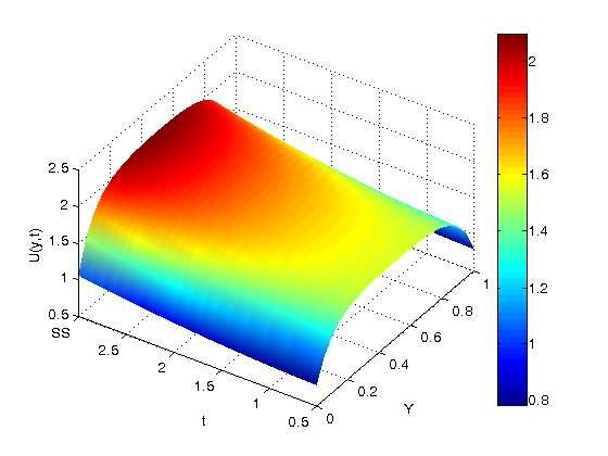
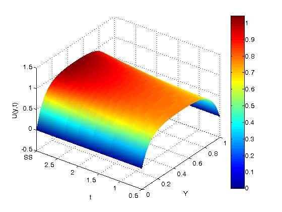
Figure 4 displays the transient velocity profile as a function of \(t\) for fixed values of the other controlling parameters. It is clear that the velocity profile rises with increasing \(t\), and that the microchannel’s center, where the maximum velocity is obtained, depends on \(t\).
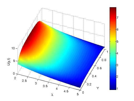
The effect of the Jeffrey parameter (\(\lambda\)) on the nanofluids’ velocity profiles is shown in Figure 5. It is graphically demonstrated that the velocity profiles decrease as the Jeffrey parameter rises, which is caused by the Jeffrey fluid elastic effect.
The effects of Darcy number (\(Da\)) on velocity profiles are shown graphically in Figure 6, where it is observed that increasing \(Da\) values result in a decrease in velocity profiles. Physically, increasing \(Da\) resists flow and enhances flow deceleration; hence, an increase in \(Da\) results in resistance to fluid motion, which lowers the velocity boundary layer and, consequently, the velocity profiles.
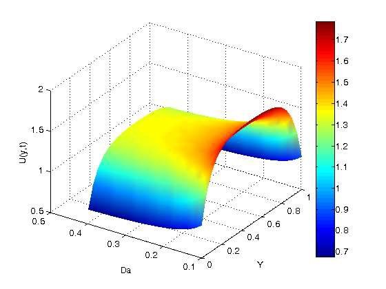
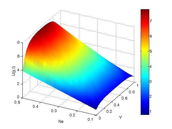
Figure 7 demonstrates the impact of the Reynolds number (\(Re\)) on velocity profiles. Graphically, it is noted that increasing the values of the Reynolds number (\(Re\)) leads to a rise in the velocity profiles, as the Reynolds number indicates the ratio of inertia force to the viscous force. Increasing the Reynolds number physically results in a decrease in the fluid’s viscous forces, which raises the velocity profiles.
Figure 8 illustrates how the magnetic parameter (\(M\)) affects velocity profiles. It can be shown graphically that the velocity profiles drop as the magnetic parameter values rise. The electromagnetic force, which is produced by the magnetic field that regulates the fluid flow characteristics, physically increases as the magnetic parameter increases. When a magnetic field is applied normal to the direction of fluid flow, it increases the Lorentz force acting against the fluid flow, causing the fluid to move more slowly and lowering its velocity. This phenomenon occurs in electrically conducting fluids.
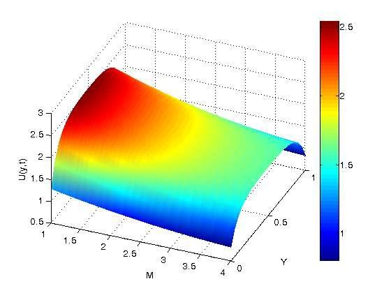
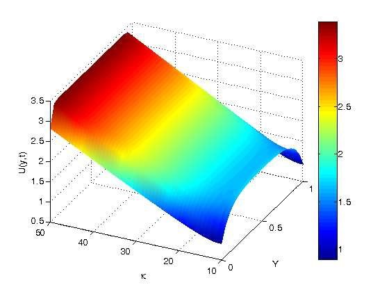
Figure 9 shows how the velocity profile is affected by the EDL size (\(K\)). Although the velocity profile is not affected by the EDL size, it can be inferred that a large EDL increases fluid flow in the center of the microchannel.
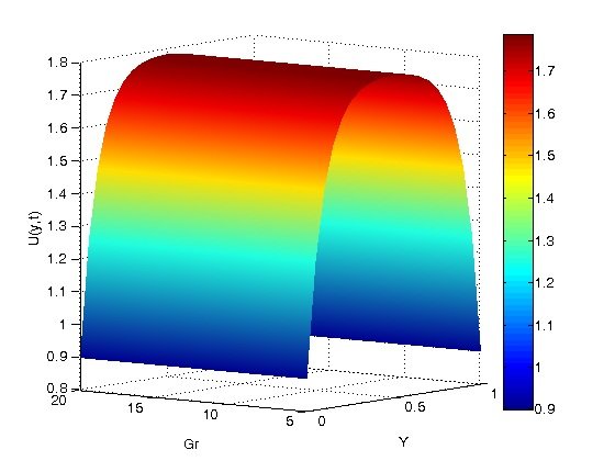
The impact of the heat transfer Grashof number (\(Gr\)) on velocity profiles is shown in Figure 10. Increasing the Grashof number for heat transfer (\(Gr\)) is shown graphically to result in an increase in the velocity profiles. The Grashof number for heat transfer is, by definition, the thermal buoyancy force divided by the viscous force. In physical terms, a higher Grashof number results in a decrease in viscous force and an increase in thermal buoyancy force, which raises velocity profiles.
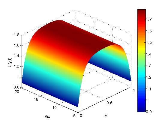
The effects of Grashof number for mass transfer (\(Gc\)) on velocity profiles are shown graphically in Figure 11, where it is observed that increasing Gc causes the fluid’s velocity to increase because Grashof number for mass transfer is the ratio of the species buoyancy force to the viscous force; physically, increasing Gc causes the fluid’s viscosity to decrease, which in turn causes a decrease in the viscous force, which in turn causes an increase in the species buoyant force and, ultimately, an increase in the fluid’s velocity.
The impact of \(\beta\) and \(t\) on the temperature distribution in the vertical microchannel is shown in Figures 12– 14. The temperature jump also rises with \(\beta\) at the wall before progressively increasing with symmetric heating throughout the microchannel to the wall. These numbers make it clear that the value of \(\beta\) is the only factor that may cause the temperature to reach a steady state. The time it takes to reach a steady state temperature is actually shortened when there is a temperature spike at the walls.
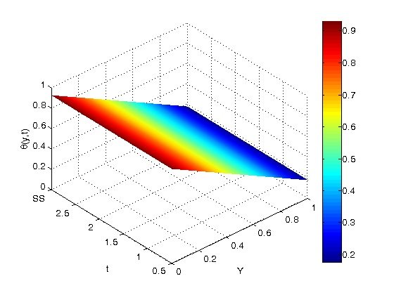
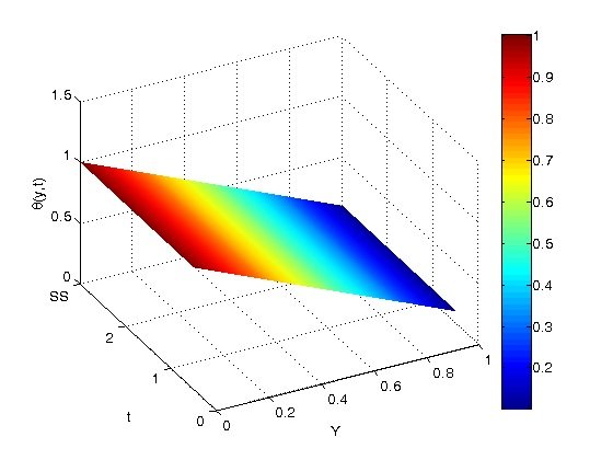
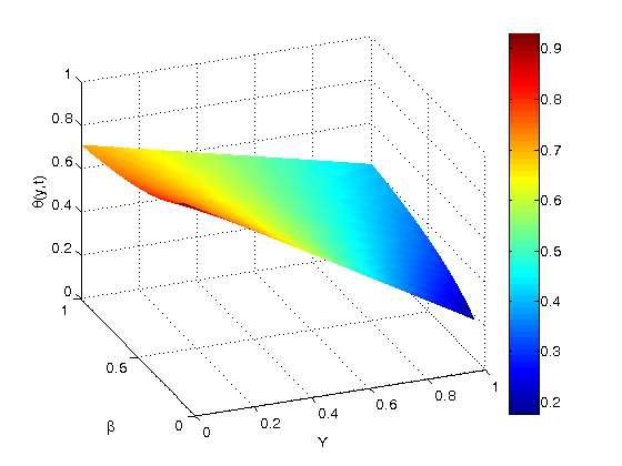
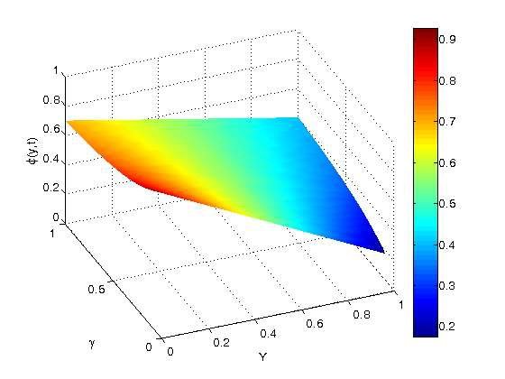
Figure 15 illustrates how \(\gamma\) and \(t\) affect the concentration in the vertical microchannel. It also shows how the concentration jumps up with \(\gamma\) near the wall before progressively increasing on the other side of the microchannel with symmetric heating.
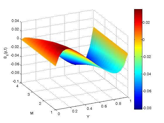
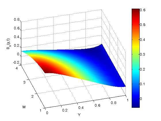
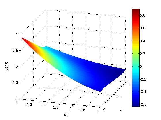
The role of the Hartmann number (\(M\)) on the dimensionless induced magnetic field in the channel is shown in Figures 16–18. For \(Y > 0.2\), the generated magnetic field increases as the Hartmann number increases, but it decreases along the plates; for \(Y = 0\) to \(Y = 1\), the induced magnetic field decreases monotonically along the plates. This is because an increase in the Hartmann number (\(M\)) increases the magnetic field strength, which in turn enhances the induced magnetic field.
Table 3 shows that, in the EMHD, EOF, nanofluid, and Jeffrey fluid model, the numerical results demonstrate that skin friction at both channel walls increases with increasing Reynolds number and EDL parameter. In the same way that a larger EDL parameter indicates a thinner electric double layer, which intensifies electroosmotic flow and boosts skin friction, higher Reynolds numbers enhance inertial effects, steepening velocity gradients near the walls and increasing shear stress. Generally, the interaction between electrokinetic forces, fluid elasticity, and nanoparticle dynamics results in a notable rise in skin friction, which is accurately captured by the numerical model. This highlights the sensitivity of wall shear to key physical parameters in complex coupled flow systems. The viscoelasticity of the Jeffrey fluid changes the flow resistance, but the combined effect of increased Re and \(\kappa\) still leads to higher wall shear. Nanoparticles contribute by increasing the fluid’s effective viscosity, further raising wall stress.
| \(K \backslash Re\) | \(U'(0)\) | \(-U'(1)\) | ||||||
|---|---|---|---|---|---|---|---|---|
| 0.1 | 0.2 | 0.3 | 0.4 | 0.1 | 0.2 | 0.3 | 0.4 | |
| 10 | 8.9921 | 17.9844 | 26.9767 | 22.7635 | 8.9918 | 17.9836 | 26.9755 | 35.9674 |
| 20 | 12.3142 | 24.6285 | 36.9428 | 45.5272 | 12.3138 | 24.6277 | 36.9417 | 49.2557 |
| 30 | 17.4159 | 34.8320 | 52.2481 | 68.2909 | 17.4156 | 34.8312 | 52.2469 | 69.6626 |
| 40 | 22.7635 | 45.5272 | 68.2909 | 91.0546 | 22.7632 | 45.5264 | 68.2897 | 91.0531 |
Table 4 shows that while the Nusselt number at the upper wall, \(\phi'(1)\), steadily rises, suggesting enhanced heat transfer at the top boundary, the Nusselt number at the lower wall, \(\phi'(0)\), gradually decreases with increasing \(t\) and axial position, suggesting a decline in heat transfer at the bottom surface over time. Overall, the heat transfer behavior shifts from a symmetric distribution to a top-biased enhancement due to evolving flow dynamics. This shift reflects the growing influence of electromagnetohydrodynamic effects and natural convection. As time progresses, the difference in trends between the two walls indicates that thermal energy is being transferred upward more efficiently.
| \(t / Re\) | \(\theta'(0)\) | \(-\theta'(1)\) | ||||||
|---|---|---|---|---|---|---|---|---|
| 0.1 | 0.2 | 0.3 | 0.4 | 0.1 | 0.2 | 0.3 | 0.4 | |
| 0.2 | 0.7410 | 0.7142 | 0.6691 | 0.6053 | 0.7509 | 0.7536 | 0.7582 | 0.7647 |
| 0.4 | 0.7462 | 0.7347 | 0.7153 | 0.6880 | 0.7513 | 0.7551 | 0.7616 | 0.7707 |
| 0.6 | 0.7487 | 0.7449 | 0.7384 | 0.7293 | 0.7538 | 0.7653 | 0.7847 | 0.8120 |
| 0.8 | 0.7491 | 0.7464 | 0.7418 | 0.7352 | 0.7590 | 0.7858 | 0.8309 | 0.8947 |
Table 5 shows the effect of the Schmidt and Reynolds numbers in the model on mass transfer, as well as the Sherwood number variation at both channel walls. A higher Schmidt number results in less mass diffusivity, which increases concentration gradients near the wall and speeds up mass transfer rates; a higher Reynolds number strengthens the convective transport of solute particles, which also raises the Sherwood number; and the presence of nanoparticles and viscoelastic effects further modifies the solute boundary layer behavior. The results show that the Sherwood number increases with both parameters, albeit moderately.
| \(Sc / Re\) | \(\phi'(0)\) | \(-\phi'(1)\) | ||||||
|---|---|---|---|---|---|---|---|---|
| 0.1 | 0.2 | 0.3 | 0.4 | 0.1 | 0.2 | 0.3 | 0.4 | |
| 0.22 | -0.7500 | -0.7582 | -0.7713 | -0.7916 | 0.7503 | 0.7584 | 0.7724 | 0.7924 |
| 0.44 | -0.7523 | -0.7593 | -0.7731 | -0.7934 | 0.7527 | 0.7597 | 0.7743 | 0.7945 |
| 0.66 | -0.7546 | -0.7602 | -0.7752 | -0.7952 | 0.7549 | 0.7614 | 0.7764 | 0.7967 |
| 0.88 | -0.7557 | -0.7623 | -0.7775 | -0.7973 | 0.7560 | 0.7634 | 0.7781 | 0.7985 |
This work examines the combined effects of velocity slip, induced magnetic field, electroosmotic flow (EOF), and Electro-Magneto-Hydrodynamic (EMHD) forces on the flow, heat, and mass transfer of a Jeffrey nanofluid confined between two parallel horizontal plates. The nanofluid is made up of copper (Cu) nanoparticles dispersed in pure water as the base fluid, and the governing nonlinear partial differential equations that account for fluid velocity, temperature, concentration, and magnetic field dynamics are solved using both the finite difference method (FDM) and the method of undetermined coefficients for steady-state analysis of the fluid.
Key dimensionless parameters, including velocity, temperature, concentration, and induced magnetic field profiles, are shown graphically. Furthermore, the impact of flow and transport parameters is illustrated through the tabulation of numerical data for the skin friction coefficient, Nusselt number, and Sherwood number.
The major findings of this work can be summarized as follows:
Nanofluid velocity increases with higher values of Grashof number (\(Gr\)), Grashof number (\(Gc\)), and permeability parameter (\(K\)), due to enhanced buoyancy and porous media effects.
An increase in the Reynolds number (\(Re\)) leads to sharper velocity gradients, thinner boundary layers, and moderately enhances both heat and mass transfer rates near the walls.
The Prandtl number (\(Pr\)) increases the Nusselt number by lowering thermal diffusivity and raising the temperature gradient and convective heat transfer at the top wall.
The Darcy number (\(Da\)) increases the velocity as well as the mass and heat transfer rates by means of fluid motion through the porous media.
Lorentz force causes a magnetic field (\(M\)) to slow fluid motion; however, it raises the produced magnetic field, especially near the lower wall, and reduces fluid velocity.
Application of velocity slip (\(\alpha\)) changes the skin friction and flow symmetry by increasing the velocity away from the boundary and lowering the shear stress near the wall.
\[\begin{aligned} N_1 &= \frac{1}{(1 – \phi + \phi \rho_s / \rho_f)} \\ N_2 &= \frac{1}{(1 – \phi + \phi \rho_s / \rho_f)(1 – \phi)^{2.5}} \\ N_3 &= ((1 – \phi) + \phi \beta_{Ts} / \beta_{Tf})) \\ N_4 &= ((1 – \phi) + \phi \beta_{Cs} / \beta_{Cf})) \\ N_5 &= \frac{1}{\left( \frac{(k_s + 2k_f) – 2\phi(k_f – k_s)}{(k_s + 2k_f) + \phi(k_f – k_s)} \right)} \\ N_6 &= \frac{1}{(1 – \phi + \phi (c_{p})_s / (c_{p})_f)} \\ N_7 &= \left( \frac{(k_s + 2k_f) – 2\phi(k_f – k_s)}{(k_s + 2k_f) + \phi(k_f – k_s)} \right) (1 – \phi + \phi (C_{p})_s / (C_{p})_f) \\ N_8 &= (1 – \phi + \phi (C_{p})_s / (C_{p})_f) \\ N_9 &= \left( \frac{(k_s + 2k_f) – 2\phi(k_f – k_s)}{(k_s + 2k_f) + \phi(k_f – k_s)} \right) (1 – \phi + \phi (C_{p})_s / (C_{p})_f) \\ N_{10} &= \left( 1 + \frac{3(\tau_1 – 1)\phi}{(\tau_1 + 2) – (\tau_1 – 1)\phi} \right) (1 – \phi + \phi (\rho C_p)_s / (\rho C_p)_f) \\ N_{11} &= \left( \frac{1}{(1 – \phi)} \frac{\mu_{eff} \varepsilon_s}{k_{eff}} \right) \\ A_1 &= \frac{1}{Re(1 + \lambda)}, \quad A_2 = \frac{N_2 D_a}{Re}, \quad A_3 = N_3 G_r, \quad A_4 = N_4 G_c, \quad A_5 = -N_1 C_1 E_z K^2, \\ A_6 &= -N_1 C_2 E_z K^2, \quad A_7 = \frac{M^2 N_1}{Re}, \quad A_8 = -N_1 \frac{dP}{dX} / Re, \quad A_9 = \frac{N_5}{Re Pr'}, \quad A_{10} = \frac{1}{Re Sc'}, \\ A_{11} &= N_{11}, \quad d_1 = 1 – \beta, \quad d_2 = 1 – \gamma, \quad d_3 = A_2 + \frac{A_7}{A_{11}}, \quad d_4 = A_3 C_7 + A_4 C_9, \quad d_5 = A_8 + A_3 C_8 + A_4 C_{10}, \\ d_6 &= \frac{d_4}{d_3}, \quad d_7 = \frac{-A_5}{A_1 K^2 – d_3}, \quad d_8 = \frac{d_5}{d_3}, \quad d_9 = \frac{d_5}{d_3}, \quad d_{10} = \frac{d_7}{d_3}, \quad m_1 = \sqrt{\frac{d_3}{A_1}}, \\ m_2 &= \sqrt{\frac{d_3}{A_1}}, \quad f_1 = \alpha m_1, \quad f_2 = 1 – \alpha m_1, \quad f_3 = e^{m_1} – \alpha m_1 e^{m_1}, \quad f_4 = e^{m_2} – \alpha m_2 e^{m_2}, \\ f_5 &= a_{1} g_8 – b_{1} g_7, \quad f_6 = a_{1} g_9 – b_{1} g_2, \quad f_7 = a_{1} g_{14} – b_{1} g_2, \quad f_8 = a_2 e^{m_1} g_8 + b_2 g_1 e^{m_1}, \\ f_9 &= a_2 e^{m_2} g_9 + b_2 g_2 e^{m_2}, \quad f_{10} = a_2 g_1 + b_2 g_9, \quad f_{11} = \alpha (d_6 + d_7 K^d – d_6 K^d) – (d_7 + d_8 + d_9), \\ f_{12} &= -\alpha (d_6 + d_7 K^d – d_6 K^d) – (d_6 + d_7 e^{K^d} + d_8 e^{-K^d}), \\ f_{13} &= -\alpha_1 (g_{11} + g_{12} + g_{13}) + b_1 (g_{8} + g_{9}) – a_2 (g_{10} – g_{11} e^{d_2} + g_{12} e^{-K^d} + g_{13}), \\ f_{14} &= b_2 (g_{3} + g_{4} e^{K^d} + g_5 e^{-K^d} + g_6) – a_2 (g_{3} + g_{4} e^{K^d} + g_5 e^{-K^d} + g_6), \\ g_1 &= \frac{-1}{A_{11}}, \quad g_2 = \frac{1}{A_{11}}, \quad g_3 = e^{m_1}, \quad g_4 = e^{-m_1}, \quad g_5 = e^{m_2}, \quad g_6 = e^{-m_2}, \\ g_7 &= g_1 + g_2, \quad g_8 = e^{m_1}, \quad g_9 = e^{-m_1}, \quad g_{10} = g_1 + g_2, \quad g_{11} = g_3 + g_4, \quad g_{12} = g_5 + g_6 \end{aligned}\]
̄ \(\phi\) Nanoparticle volume
fraction
\(Sc\) Schmidt number
\(T\) Temperature (K)
\(C\) Species concentration
(mole/kg)
\(C_p\) Specific heat at constant
pressure (J kg\(^{-1}\) K\(^{-1}\))
\(E'_x\) Applied electric field in
x-direction
\(E_x\) Applied electric field in
x-direction (Dimensionless)
\(T_w\) Temperature of the fluid in the
moving plate (K)
\(T_0\) Temperature of the fluid in the
stationary plate (K)
\(C_w\) Concentration of the fluid in
the moving plate (mole/kg)
\(h\) Distance between two parallel
plates (m)
\(B_x\) Non-dimensional induced
magnetic field
\(u\) Dimensionless velocity
(m/s)
\(u'\) Dimensional velocity
(m/s)
\(U\) Constant reference velocity
\(\mu\) Viscosity (kg m\(^{-1}\) s\(^{-1}\))
\(\rho\) Fluid density (kg m\(^{-3}\))
\(\sigma\) Electrical conductivity
(S/m)
\(\theta\) Non-dimensional
temperature
\(\phi\) Non-dimensional
concentration
\(\nu\) Kinematic viscosity (m\(^2\)/s)
\(\mu_e\) Magnetic permeability
\(\kappa\) Debye-Huckel parameter
\(K\) Debye-Huckel parameter
(Dimensionless)
\(C_0\) Concentration of the fluid in
the stationary plate (mole/kg)
\(D_m\) Mass diffusivity / Chemical
molecular diffusivity (m\(^2\)/s)
\(g\) Acceleration due to gravity
(m/s\(^2\))
\(B_0\) Uniform applied magnetic field
along x-axis
\(K\) Coefficient of thermal
conductivity (W/m·K)
\(t'\) Time (s)
\(t\) Dimensionless time
\(B_x\) Induced magnetic field along
x-direction (T)
\(J\) Current density (A/m\(^2\))
\(\vec{B}\) Magnetic field strength
(A/m)
\(C_s\) Concentration susceptibility
(m/mole)
\(C_m\) Mean concentration
(m/mole)
\(T_m\) Mean fluid temperature
(K)
\(K_t\) Thermal diffusion ratio
\(M\) Magnetic parameter
\(Re\) Reynolds number
\(Da\) Permeability parameter
\(Pr\) Prandtl number
\(\beta_T\) Coefficient of volume
expansion due to temperature
\(\beta_c\) Coefficient of volume
expansion due to concentration
\(\rho_e\) Charge density
\(nf\) Nanofluid
\(f\) Fluid
\(s\) Solid
\(\lambda\) Jeffrey parameter
\(\varepsilon\) Fluid permittivity
(dimensionless)
\(\xi', \xi'_1, \xi'_2\)
Zeta potential (electrokinetic potential of the walls in the double
layer)
\(\xi, \xi_1, \xi_2\) Zeta potential
(Dimensionless)