
The study of transient free convective flow in vertical channels plays a critical role in understanding heat and mass transfer processes across various scientific and engineering applications, including energy systems, environmental engineering, and industrial processes. Free convection, driven by buoyancy forces resulting from temperature gradients, is a fundamental mechanism for fluid motion and heat exchange in such systems. When coupled with complex boundary conditions, such as third-kind (Robin-type) thermal boundaries, the analysis becomes not only analytically challenging but also highly relevant to real world scenarios.
Thermal boundary conditions of the third kind where heat transfer occurs via convective exchange between the fluid and its surroundings are particularly important for modeling practical systems such as heat exchangers, cooling devices, and insulated channels. In such systems, the heat flux depends on the temperature difference and a convective heat transfer coefficient, offering a more realistic representation compared to idealized isothermal or adiabatic conditions.
This study adopts a semi-analytical approach to investigate the transient free convection flow of a viscous, incompressible fluid within a vertical channel subject to third-kind thermal boundary conditions. It also addresses inverse thermal problems involving boundary conditions previously criticized by Javeri [1] and Cioffalo [2]. The Laplace transform technique is employed to obtain solutions in the Laplace domain, which are subsequently inverted numerically to yield time-dependent results. To generalize the classical model and account for memory and hereditary effects in complex fluid flows, fractional derivatives specifically the Caputo-Fabrizio and Atangana-Baleanu models are incorporated.
The primary aim of this study is to analyze the transient behavior of the flow and heat transfer characteristics, including temperature distribution, velocity profiles, Nusselt number, and shear stress. The semi-analytical results, validated through MATLAB computations, provide insight into the influence of thermal boundary conditions, fractional parameters, and other governing factors on the fluid flow.
Several prior studies have explored similar themes. Sergio and Ramos [3] investigated heat transfer in MHD channel flow under third-kind boundary conditions. Kumar et al. [4] examined mixed convective heat transfer of immiscible fluids in a vertical channel subject to third-kind boundary conditions. Javeri [5] scrutinized the influence of Hall current, ion slip, and third-kind thermal boundaries in MHD flows, while Cuevas and Ramos [6] conducted a thermal analysis of MHD flow under similar conditions. Ren et al. [7] employed an immersed boundary method for thermal flows with Dirichlet temperature constraints, and Rosales-Vera [8] presented a semi-analytical solution of the Cartesian Graetz problem with convective third-kind boundary conditions.
Zare et al. [9] provided analytical and numerical solutions of transient heat conduction in infinite domains with internal heat generation and heterogeneous third-kind boundaries. Hajji-Sheikh and Lakshminarayanan [10] used an integral approach to treat second- and third-kind boundary conditions in diffusion problems. Peter [11] discussed monotone, high-order accurate schemes for differential equations with these boundary types. Siddheshwar et al. [12] studied Brinkman–Bénard convection in domains with surface roughness and third-kind boundaries, and Shahnazari et al. [13] proposed a perturbative method for converting third-type into first-type boundary conditions.
Gladwell et al. [14] analyzed heat transfer under radiation boundary conditions, while Mahdavi et al. [15] conducted an integrated experimental-numerical study on natural convection in a water-filled enclosure, emphasizing boundary condition optimization and transient magnetohydrodynamic flow. The significance of transient free convection between infinite vertical parallel surfaces cannot be overstated due to its applications in various technological processes, including the early stages of melting and transient heating of insulating air gaps, such as during incinerator startup.
Singh et al. [16] and Joshi [17] explored transient free convection between asymmetrically heated infinite vertical plates and the natural convection cooling of vertical walls, respectively. Jha et al. [18] examined symmetric heating, and Paul et al. [19, 20] investigated isothermal, isoflux, and combined boundary effects on vertical channels. Ajibade and Jha [21, 22] studied flows with temperature-dependent heat sources and sinks. Applications of unsteady natural convection include internal cooling of nuclear reactors, failure scenarios in power systems, and temperature regulation of electronic components.
Aung et al. [23, 24] investigated laminar flows in vertical channels under asymmetric heating, while Terekhov and Ekaid [25] used a finite volume method to analyze natural convection between asymmetrically heated walls. Al-Nimr and El-Shaarawi [26] focused on fully developed transient natural convection, and Paul and sigh [27] addressed asymmetric heating and cooling. Sarkar et al. [28] analyzed asymmetric transient MHD convection, and Mandal et al. [29] studied radiation effects. Buonomo and Manca [30] evaluated transient convection in micro-channels with uniform heat flux, and Rajput and Sahu [31] investigated transient MHD convection between vertical plates with variable mass diffusion.
The present work aims to develop a closed-form solution for generalized fractional time derivatives governing natural convection between two infinite vertical plates, with one plate isothermally heated. The governing partial differential equations are transformed into ordinary differential equations using the Laplace transform method. Closed-form solutions in the Laplace domain are obtained and inverted to the time domain using the Riemann-sum approximation. The effects of flow parameters such as Biot number, buoyancy force, and Prandtl number on temperature distribution, velocity profiles, Nusselt number, and skin friction are presented both graphically and in tabular form.
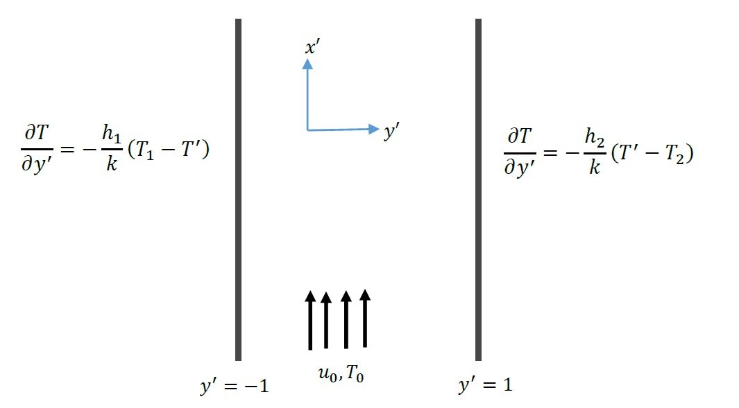
Consider the transient free-convective flow of viscous incompressible fluid between two infinite vertical parallel plates separated by a distance \(h\). The \(x\)-axis is taken along one of the plates and \(y\)-axis is taken normal to the plate, as shown in Figure 1. Initially, the temperature of the plates and the fluid is assumed to be \(T_0\). One of the plate start moving at \(t>0\) in its own plane while the other plate at distance \(h\) is kept fixed. The transient motion of the fluid is caused by the buoyancy force arising from the temperature gradient as a result of constant temperature on one plate \((y=h)\) and adiabatic condition on the other plate \((y=1)\). Then, the flow can be governed by the dimensional forms of equations under usual Boussinesq’s approximation:
\[ \frac{\partial u'}{\partial t'} = \nu \frac{\partial^2 u'}{\partial y'^2} + g\beta(T' – T_0) \label{eq1}, \ \tag{1}\] \[ \frac{\partial T'}{\partial t'} = \alpha \frac{\partial^2 T'}{\partial y'^2}. \label{eq2} \tag{2}\]
With initial and boundary conditions: \[t' \leq 0 : \quad u' = 0, \quad T' = T_0 \quad \text{for } -d \leq y \leq d, \quad 0 < \eta < 1,\]
\[\label{eq3} \begin{cases} t' > 0 :\quad u' = 0 \\ \quad \left. \frac{\partial T'}{\partial y'} \right|_{y' = -d} = \frac{-h_1}{k}(T_1 – T') ,\\ \quad \left. \frac{\partial T'}{\partial y'} \right|_{y' = +d} = \frac{-h_2}{k}(T' – T_2). \end{cases} \tag{3}\]
By introducing non-dimensional quantities \[\label{eq4} \theta = \frac{T' – T_0}{T_1 – T_0}, \quad Rt = \frac{T_2 – T_0}{T_1 – T_0}, \quad y = \frac{y'}{\lambda}, \quad t = \frac{t' \nu}{\lambda^2}, \quad \text{Pr} = \frac{\nu}{\alpha} . \tag{4}\]
Let \(u = u' \left[ \nu g \beta (T_1 – T_0) d^2 \right]^{-1}\) for \(0 < \eta < 1\), Eqs (1) and (2) become
\[ \frac{\partial u}{\partial t} = \frac{\partial^2 u}{\partial y^2} + \theta ,\label{eq5} \ \tag{5}\] \[ \frac{\partial \theta}{\partial t} = \frac{1}{\text{Pr}} \frac{\partial^2 \theta}{\partial y^2}. \label{eq6} \tag{6}\]
Subject to initial and boundary conditions:
\[t \leq 0: \quad u = 0, \quad \theta = 0 \quad \text{for } -1 \leq y \leq 1,\]
\[\label{eq7} t > 0: \quad \begin{cases} u = 0, \quad \dfrac{\partial \theta}{\partial y} = B_{i1} (\theta – 1), & \text{at } y = -1 ,\\ u = 0, \quad \dfrac{\partial \theta}{\partial y} = B_{i2} (Rt – \theta), & \text{at } y = +1. \end{cases} \tag{7}\]
It is clearly known that the parameter \(Rt\) is very significant due to its fundamental effect on the fluid flow process between the vertical walls. This parameter essentially repairs the orientation of the fluid temperature \(T_0\) with respect to the vertical wall temperature \(T_2\) and \(T'\).
Case I. Classical case
Introducing the Laplace transform of the dimensionless velocity and temperature \[\bar{u}(y,s) = \int_{0}^{\infty} u(y,t)\exp(-st)\,dt \quad \text{and} \quad \bar{T}(y,s) = \int_{0}^{\infty} T(y,t)\exp(-st)\,dt,\] (where \(s\) is the Laplace parameter) and by deploying the properties of Laplace transform in (3), Eqs. (1) and (2) are subject to initial condition given
\[\label{eq8} \frac{d^2 \bar{u}}{dy^2} – s \bar{u} = -\theta, \tag{8}\]
\[\label{eq9} \frac{d^2 \bar{\theta}}{dy^2} = \text{Pr} \, s \, \bar{\theta} . \tag{9}\]
Then Eq. (3) can be written as \[\begin{aligned} \label{eq10} \bar{u} =& 0, \quad \frac{d \bar{T}}{dy} = 0 \quad \text{at } y = -1 ,\notag\\ \bar{u} =& 0, \quad Rt = \bar{T} = \frac{1}{s} \quad \text{at } y = 1 . \end{aligned} \tag{10}\]
The solution of the Eqs. (8) and (9) subject to boundary condition (10) can be written as \[\begin{aligned} \label{eq11} \bar{u}(y,s) =& \frac{1}{s(\text{Pr} – 1)} \left[ \frac{ c_1 \left( \cosh(\sqrt{s \, \text{Pr}}) \cosh(y \sqrt{s}) – \cosh(y \sqrt{s \, \text{Pr}}) \cosh(\sqrt{s}) \right) }{\cosh(\sqrt{s})}\right.\notag\\ &\left.+ \frac{ c_2 \left( \sinh(\sqrt{s \, \text{Pr}}) \sinh(y \sqrt{s}) – \sinh(y \sqrt{s \, \text{Pr}}) \sinh(\sqrt{s}) \right) }{\sinh(\sqrt{s})} \right], \end{aligned} \tag{11}\] \[\label{eq12} \bar{\theta}(y,s) = c_1 \cosh(y \sqrt{s \, \text{Pr}}) + c_2 \sinh(y \sqrt{s \, \text{Pr}}). \tag{12}\]
Eq. (11) and (12) are differentiated with respect to y to obtain the skin friction and Nusselt number then we have
\[\begin{aligned} \label{eq13} \frac{d \bar{u}}{dy} =& \frac{1}{s(\text{Pr} – 1)} \left[ \frac{c_1 \left( \sqrt{s} \cosh(\sqrt{s \, \text{Pr}}) \sinh(y \sqrt{s}) – \sqrt{s \, \text{Pr}} \sinh(y \sqrt{s \, \text{Pr}}) \cosh(\sqrt{s}) \right)}{\cosh(\sqrt{s})}\right.\notag\\ &\left.+ \frac{c_2 \left( \sqrt{s} \sinh(\sqrt{s \, \text{Pr}}) \cosh(y \sqrt{s}) – \sqrt{s \, \text{Pr}} \cosh(y \sqrt{s \, \text{Pr}}) \sinh(\sqrt{s}) \right)}{\sinh(\sqrt{s})} \right] , \end{aligned} \tag{13}\]
\[\label{eq14} \bar{\theta}(y,s) = c_1 \sqrt{s \, \text{Pr}} \sinh(y \sqrt{s \, \text{Pr}}) + c_2 \sqrt{s \, \text{Pr}} \cosh(y \sqrt{s \, \text{Pr}}). \tag{14}\]
Case II. Caputo–Fabrizio Model
The solutions for velocity and temperature in Caputo–Fabrizio time derivative are
\[\begin{aligned} \label{eq15} \bar{u}(y,s) =& \frac{(1 – \eta + \eta)}{s(\text{Pr} – [(1 – \eta)s + \eta])}\notag\\ &\times\left[ \frac{ c_1 \left( \cosh\left( \sqrt{ \frac{s\, \text{Pr}}{(1 – \eta)s + \eta} } \right) \cosh\left( y \sqrt{ \frac{s}{(1 – \eta)s + \eta} } \right) – \cosh\left( \sqrt{ \frac{s\, \text{Pr}}{(1 – \eta)s + \eta} } \right) \cosh\left( \sqrt{s} \right) \right) }{\cosh(\sqrt{s})}\right.\notag\\ &\left.+ \frac{ c_2 \left( \sinh\left( \sqrt{ \frac{s\, \text{Pr}}{(1 – \eta)s + \eta} } \right) \sinh\left( y \sqrt{ \frac{s}{(1 – \eta)s + \eta} } \right) – \sinh\left( \sqrt{ \frac{s\, \text{Pr}}{(1 – \eta)s + \eta} } \right) \sinh\left( \sqrt{s} \right) \right) }{\sinh(\sqrt{s})} \right], \end{aligned} \tag{15}\]
\[\label{eq16} \bar{\theta}(y,s) = c_1 \cosh\left( y \sqrt{ \frac{s\, \text{Pr}}{(1 – \eta)s + \eta} } \right) + c_2 \sinh\left( y \sqrt{ \frac{s\, \text{Pr}}{(1 – \eta)s + \eta} } \right). \tag{16}\]
Differentiating (15) and (16) with respect to \(y\) we have
\[\begin{aligned} \label{eq17} \frac{d\bar{u}}{dy}&(y,s) = \frac{(1 – \eta + \eta)}{s(\text{Pr} – [(1 – \eta)s + \eta])}\notag\\ &\times\left[ \frac{ c_1 \left( \sqrt{ \frac{s}{(1 – \eta)s + \eta} } \cosh\left( \sqrt{ \frac{s\, \text{Pr}}{(1 – \eta)s + \eta} } \right) \sinh\left( y \sqrt{ \frac{s}{(1 – \eta)s + \eta} } \right) – \sqrt{ \frac{s\, \text{Pr}}{(1 – \eta)s + \eta} } \sinh\left( y \sqrt{ \frac{s\, \text{Pr}}{(1 – \eta)s + \eta} } \right) \cosh(\sqrt{s}) \right) }{\cosh(\sqrt{s})}\right.\notag\\ &\left. + \frac{ c_2 \left( \sqrt{ \frac{s}{(1 – \eta)s + \eta} } \sinh\left( \sqrt{ \frac{s\, \text{Pr}}{(1 – \eta)s + \eta} } \right) \cosh\left( y \sqrt{ \frac{s}{(1 – \eta)s + \eta} } \right) – \sqrt{ \frac{s\, \text{Pr}}{(1 – \eta)s + \eta} } \cosh\left( y \sqrt{ \frac{s\, \text{Pr}}{(1 – \eta)s + \eta} } \right) \sinh(\sqrt{s}) \right) }{\sinh(\sqrt{s})} \right], \end{aligned} \tag{17}\]
\[\label{eq18} \bar{\theta}(y,s) = c_1 \sqrt{ \frac{s\, \text{Pr}}{(1 – \eta)s + \eta} } \sinh\left( y \sqrt{ \frac{s\, \text{Pr}}{(1 – \eta)s + \eta} } \right) + c_2 \sqrt{ \frac{s\, \text{Pr}}{(1 – \eta)s + \eta} } \cosh\left( y \sqrt{ \frac{s\, \text{Pr}}{(1 – \eta)s + \eta} } \right). \tag{18}\]
Case III. Atangana–Baleanu Time Derivative Model
The solutions for velocity and temperature in Atangana–Baleanu time derivative are:
\[\begin{aligned} \label{eq19} \bar{u}(y,s) =& \frac{(1 – \eta) s^\gamma + \eta}{s^\gamma \left( \text{Pr} – [(1 – \eta) s^\gamma + \eta] \right)} \notag\\ &\times\left[ \frac{ c_1 \left( \cosh\left( \sqrt{ \frac{s^\gamma \text{Pr}}{(1 – \eta) s^\gamma + \eta} } \right) \cosh\left( y \sqrt{ \frac{s^\gamma}{(1 – \eta) s^\gamma + \eta} } \right) – \cosh\left( \sqrt{ \frac{s^\gamma \text{Pr}}{(1 – \eta) s^\gamma + \eta} } \right) \cosh\left( \sqrt{s^\gamma} \right) \right) }{\cosh\left( \sqrt{s^\gamma} \right)}\right.\notag\\ &\left. + \frac{ c_2 \left( \sinh\left( \sqrt{ \frac{s^\gamma \text{Pr}}{(1 – \eta) s^\gamma + \eta} } \right) \sinh\left( y \sqrt{ \frac{s^\gamma}{(1 – \eta) s^\gamma + \eta} } \right) – \sinh\left( \sqrt{ \frac{s^\gamma \text{Pr}}{(1 – \eta) s^\gamma + \eta} } \right) \sinh\left( \sqrt{s^\gamma} \right) \right) }{\sinh\left( \sqrt{s^\gamma} \right)} \right], \end{aligned} \tag{19}\]
\[\label{eq20} \bar{\theta}(y,s) = c_1 \cosh\left( y \sqrt{ \frac{s^\gamma \text{Pr}}{(1 – \eta) s^\gamma + \eta} } \right) + c_2 \sinh\left( y \sqrt{ \frac{s^\gamma \text{Pr}}{(1 – \eta) s^\gamma + \eta} } \right). \tag{20}\]
\[\begin{aligned} \label{eq21} &\frac{d \bar{u}}{dy}(y,s) = \frac{(1 – \eta)s^\gamma + \eta}{s^\gamma \left( \text{Pr} – [(1 – \eta)s^\gamma + \eta] \right)}\notag\\ &\times\left[ \frac{ c_1 \left( \sqrt{ \frac{s^\gamma}{(1 – \eta)s^\gamma + \eta} } \cosh\left( \sqrt{ \frac{s^\gamma \text{Pr}}{(1 – \eta)s^\gamma + \eta} } \right) \sinh\left( y \sqrt{ \frac{s^\gamma}{(1 – \eta)s^\gamma + \eta} } \right) – \sqrt{ \frac{s^\gamma \text{Pr}}{(1 – \eta)s^\gamma + \eta} } \sinh\left( y \sqrt{ \frac{s^\gamma \text{Pr}}{(1 – \eta)s^\gamma + \eta} } \right) \cosh\left( \sqrt{s^\gamma} \right) \right) }{\cosh\left( \sqrt{s^\gamma} \right)}\right.\notag\\ &\left. + \frac{ c_2 \left( \sqrt{ \frac{s^\gamma}{(1 – \eta)s^\gamma + \eta} } \sinh\left( \sqrt{ \frac{s^\gamma \text{Pr}}{(1 – \eta)s^\gamma + \eta} } \right) \cosh\left( y \sqrt{ \frac{s^\gamma}{(1 – \eta)s^\gamma + \eta} } \right) – \sqrt{ \frac{s^\gamma \text{Pr}}{(1 – \eta)s^\gamma + \eta} } \cosh\left( y \sqrt{ \frac{s^\gamma \text{Pr}}{(1 – \eta)s^\gamma + \eta} } \right) \sinh\left( \sqrt{s^\gamma} \right) \right) }{\sinh\left( \sqrt{s^\gamma} \right)} \right], \end{aligned} \tag{21}\]
\[\label{eq22} \bar{\theta}(y,s) = c_1 \sqrt{ \frac{s^\gamma \, \text{Pr}}{(1 – \eta)s^\gamma + \eta} } \sinh\left( y \sqrt{ \frac{s^\gamma \, \text{Pr}}{(1 – \eta)s^\gamma + \eta} } \right) + c_2 \sqrt{ \frac{s^\gamma \, \text{Pr}}{(1 – \eta)s^\gamma + \eta} } \cosh\left( y \sqrt{ \frac{s^\gamma \, \text{Pr}}{(1 – \eta)s^\gamma + \eta} } \right), \tag{22}\] where
\[\label{eq23} c_1 = \frac{1}{s} \cdot \frac{a_1 B_{i2} \times Rt + a_2 \times B_{i1}}{a_1 \times a_4 + a_2 \times a_3}, \quad \text{and}\quad c_2 = \frac{1}{s} \cdot \frac{B_{i2} \times Rt \times a_2 – B_{i1} \times a_4}{a_3 \times a_2 + a_1 \times a_4}. \tag{23}\]
The velocity and temperature distributions obtained from Eqs. (11)-(12) are to be inverted to the time domain. But these inversions cannot be easily obtained in closed-form, hence we employed the use of a numerical procedure used by [32] which is based on the Riemann-sum approximation (RSA) method. This Laplace inversion procedure based on RSA for velocity and temperature is as follows:
\[\label{eq24} u(y,t) = e^{\frac{\epsilon t}{2}} \left[ \frac{1}{2} \bar{u}(y,\epsilon) + \text{Re} \sum_{k=1}^{N^*} \bar{u}\left(y, \epsilon + \frac{ik\pi}{t} \right)(-1)^k \right], \tag{24}\]
\[\label{eq25} \theta(y,t) = e^{\frac{\epsilon t}{2}} \left[ \frac{1}{2} \bar{\theta}(y,\epsilon) + \text{Re} \sum_{k=1}^{N^*} \bar{\theta}\left(y, \epsilon + \frac{ik\pi}{t} \right)(-1)^k \right], \tag{25}\] where \(N\) is the number of terms used in the Riemann-sum approximation (RSA), \(\epsilon\) is the real part of the Bromwich contour that is used in inverting Laplace transforms and \(\text{Re}\) refers to the real part of the imaginary number \(i\). The RSA for the Laplace inversion involves a single summation for the numerical process. The correctness of this method depends on the value of \(\epsilon\) and its truncation error dictated by \(N\). Based on numerical experimentation and according to Tzou [33], the value of \(\epsilon\) must be selected so that the Bromwich contour encompasses all the branch points. For quicker convergence, the quantity \(\epsilon\,t = 4.7\) gives the most satisfactory results.
In this current work, we applied MATLAB software to validate the accuracy of Riemann sum approximation (RSA) method with the work of [34] by comparing the numerical values of the dimensionless velocity, skin friction and Nusselt number.
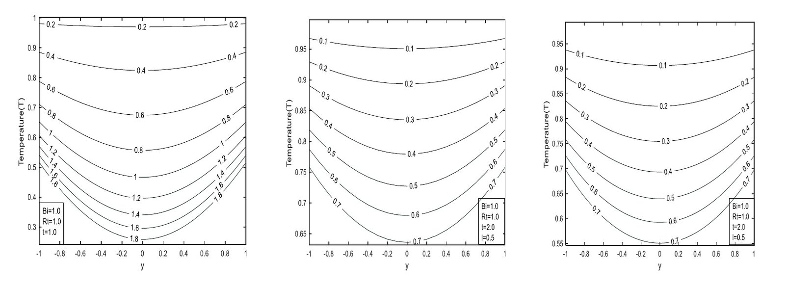
Figure 2 shows the effect of the buoyancy force parameter Rt on the temperature field. It is observed that the fluid temperature increases with an increase in buoyancy force for both air and water across the classical, Caputo–Fabrizio (CF), and Atangana–Baleanu (ABC) models. The classical model exhibits a sharper increase in temperature with thermal radiation Rt, indicating faster heat diffusion without memory effects. In contrast, the CF and ABC models show more gradual temperature rises due to their inherent nonlocal and memory-dependent characteristics. Specifically, the ABC model exhibits the highest temperature retention away from the wall, indicating stronger thermal memory effects and slower diffusion.
These results imply that the classical model is suitable for immediate thermal responses in conventional systems; the CF model is applicable to transient heat conditions in advanced materials with moderate memory effects; and the ABC model, characterized by long-term memory effects, is ideal for complex applications such as nanofluid flow in biomedical engineering, high-performance electronics cooling, and thermal management in space systems.
Figure 3 shows that fluid temperature also increases with time; however, this increase is less pronounced in air than in water for both fractional models (ABC and CF). The classical model remains more suitable for fast-response heating systems, whereas the CF and ABC models provide superior realism for transient or memory-sensitive systems, such as aerospace surfaces and biomedical thermal management. The buoyancy-driven mixed convection intensifies with increasing temperature over time, influencing flow patterns and system stability.
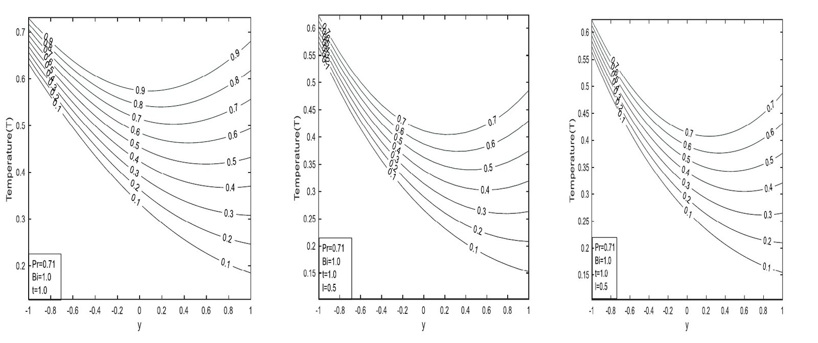
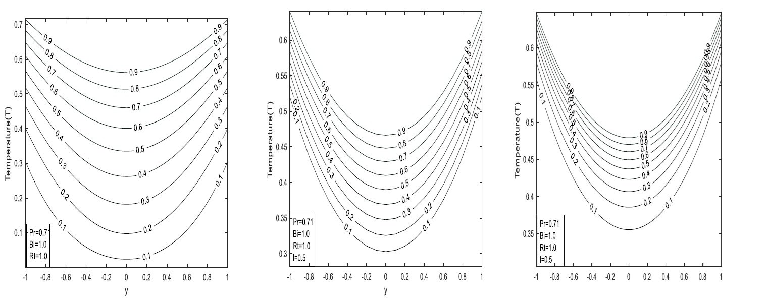
Figure 4 illustrates the effect of the Biot number, showing that fluid temperature increases as the Biot number increases. Figure 5 demonstrates the impact of the Prandtl number Pr on temperature: fluid temperature and thermal boundary layer thickness decrease with increasing Pr values. Physically, this is more prominent at low Pr values, where higher thermal conductivity allows heat to dissipate rapidly from the wall. For the classical model, higher Pr leads to steeper temperature gradients, whereas lower Pr results in flatter profiles. This model applies well to conventional fluids like oils and gases.
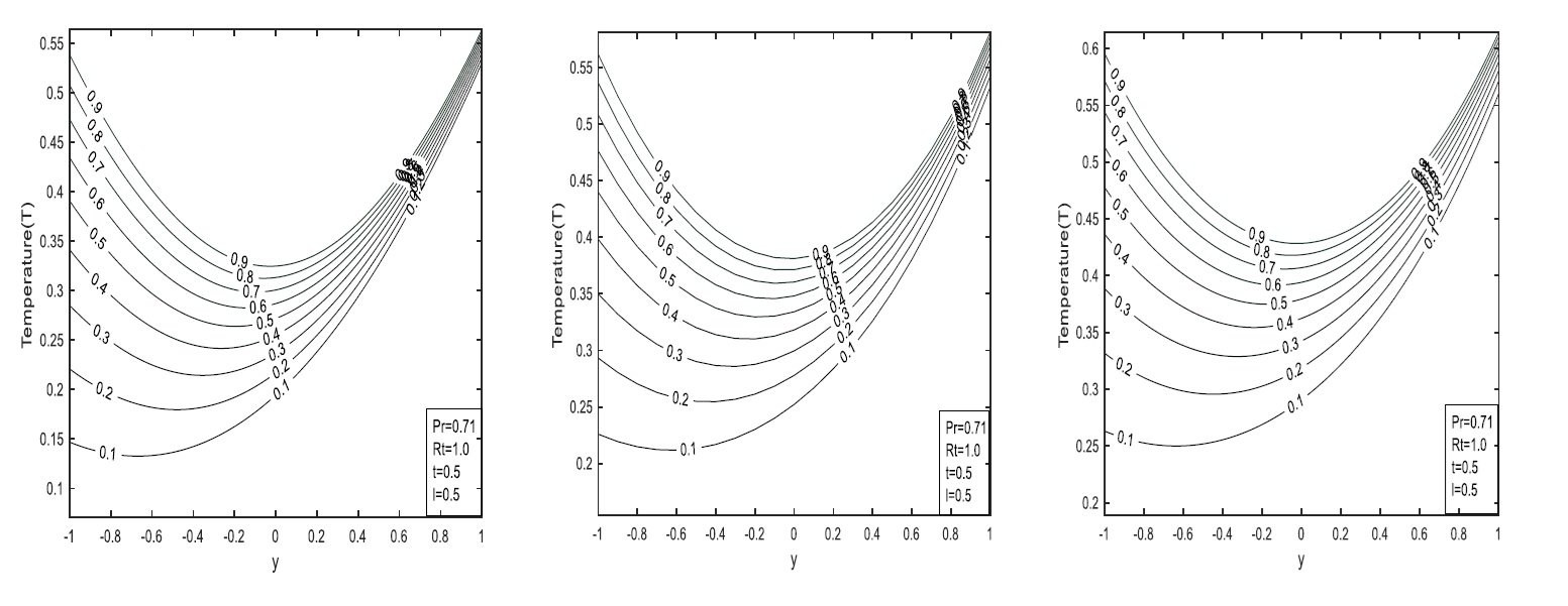
The CF model produces smoother temperature profiles with moderate gradients compared to the classical case due to its mild memory effects. The temperature profile flattens as Pr decreases, reflecting slower heat propagation. This model is suitable for systems with short-term memory, such as biological tissues or polymers. The ABC model yields the flattest temperature profiles, attributable to pronounced memory effects, exhibiting the slowest thermal response among the three models. Its nonlocal, anomalous diffusion behavior makes it ideal for applications like porous media and anomalous conduction.
Figure 6 shows the effect of the buoyancy force Rt on the fluid flow rate, measured by the Nusselt number Nu. The flow rate increases with increasing buoyancy force for both walls. The classical derivative produces a steep decline in Nu, indicating purely local, memory-less heat transfer behavior. The CF derivative shows a more gradual reduction, capturing short-term memory effects and representing a moderate thermal response, while the ABC derivative results in the most gradual increase, effectively characterizing long-term memory effects in heat transfer.
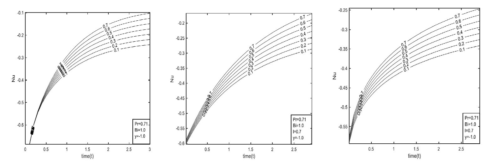
Figure 7 illustrates the effect of the Biot number on the flow rate. An increase in Bi correlates with a decrease in the flow rate, with convergence observed near y=1.0. The classical model yields the highest Nusselt numbers, while the ABC model yields the lowest, highlighting the differing complexities and underlying assumptions of each formulation. The CF and ABC models incorporate more realistic and intricate heat transfer mechanisms than the classical approach. These models are particularly relevant in applications where boundary thermal resistance significantly influences heat exchange efficiency.
Figure 8 presents the effect of the Prandtl number on fluid flow rate, showing that an increase in Pr corresponds to a rise in flow rate. Although a higher Pr generally indicates decreased thermal diffusivity relative to kinematic viscosity implying slower heat transfer in this case, it is associated with higher Nusselt numbers and stronger convective heat transfer.
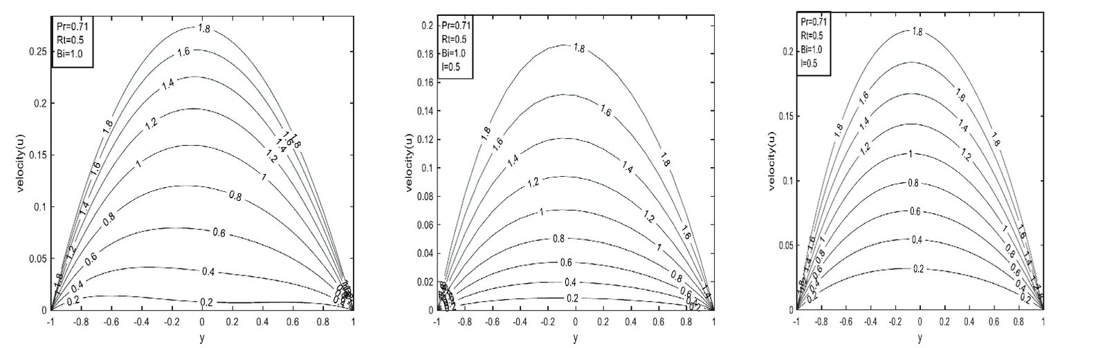
Figure 9 illustrates the effect of buoyancy force on fluid velocity. Increasing Rt induces rapid growth in fluid velocity, reflecting enhanced thermal energy driving fluid motion. All models display parabolic and symmetric velocity profiles, with the classical model exhibiting the highest peak, indicating a strong and immediate response to thermal radiation.
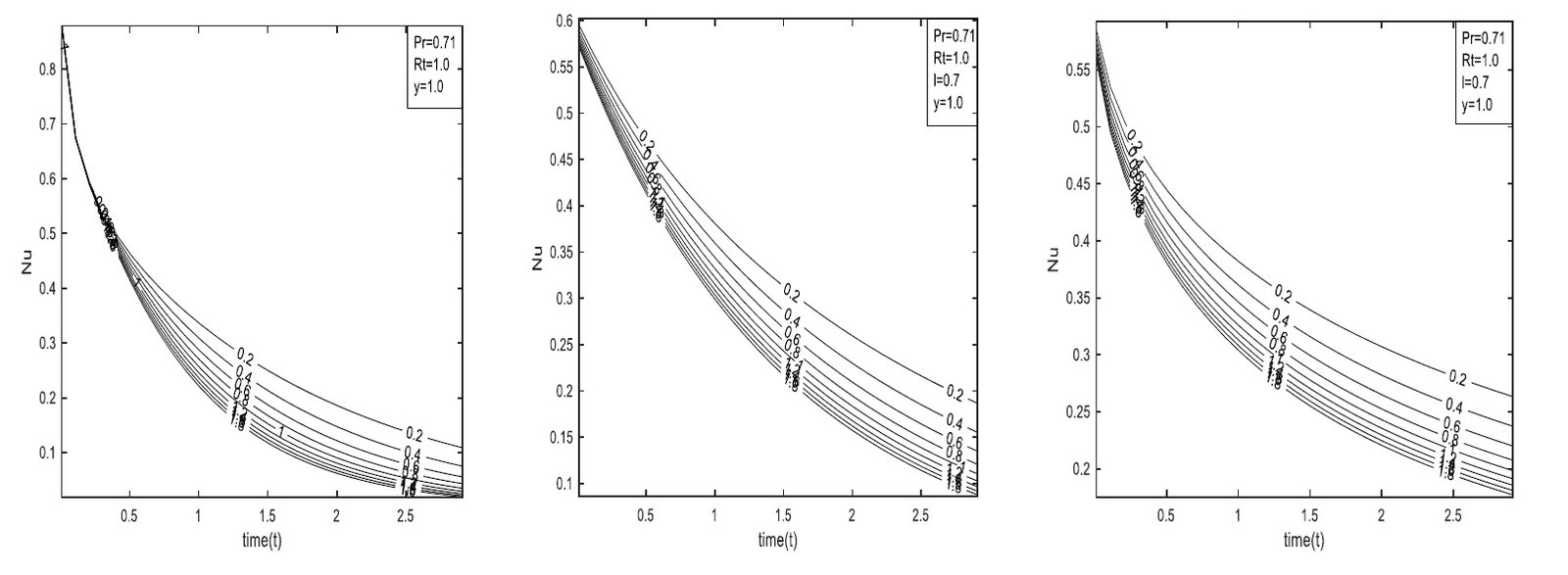
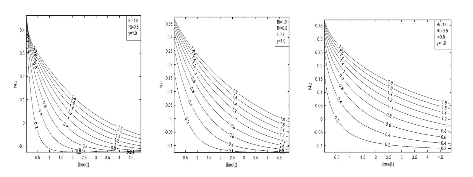
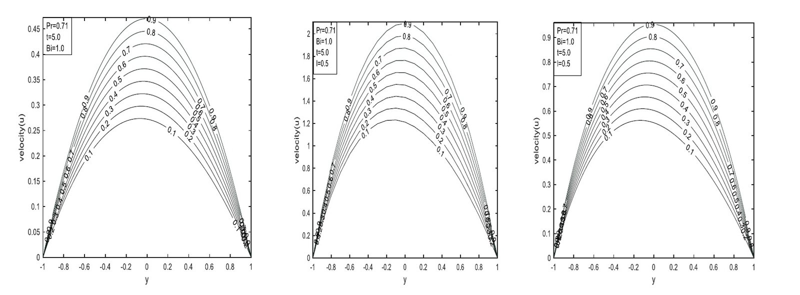
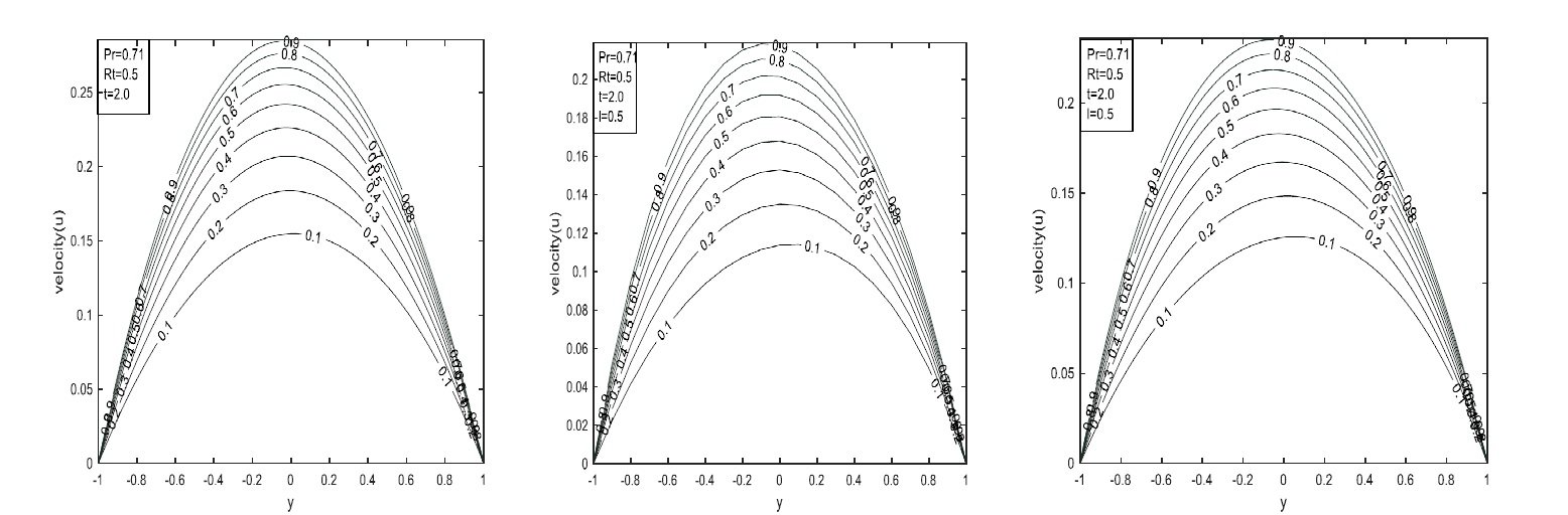
Figure 10 shows the influence of time on velocity for all models. The ABC fractional model consistently shows greater velocity than the CF and classical models. The classical model displays the highest velocity peaks and is more suitable for basic applications, while the CF and ABC models reach lower maxima, indicating varying rates of flow development. These fractional models are better suited for time-dependent systems where memory effects influence motion dynamics. The figure suggests that a steady-state velocity may be reached at sufficiently large times.
Figure 11 demonstrates the effect of the Biot number on velocity profiles. Fluid velocity increases with Bi, with all models showing a corresponding increase, indicating enhanced surface heat transfer. The classical model assumes instantaneous local diffusion, making it suitable for simple Newtonian flows. The CF model, using an exponential memory kernel, better captures fluids with moderate viscoelastic behavior. The ABC model, with its Mittag–Leffler kernel, is more appropriate for complex or biological systems such as porous media or anomalous heat transfer, where long-term memory significantly affects flow.
As Pr increases, fluid velocity decreases due to the higher viscosity and lower thermal conductivity associated with larger Pr values. Physically, a higher Prandtl number implies reduced thermal diffusion and a more viscous fluid, leading to a thicker momentum boundary layer and slower near-surface velocity. In the classical model, the fluid accelerates more freely, resulting in higher velocities. The CF and ABC models incorporate fractional derivatives with memory kernels that introduce damping effects, slowing the fluid flow more significantly as Pr increases. The CF model shows moderate damping, while the ABC model exhibits the strongest damping due to its heavier memory impact, as illustrated in Figure 12.
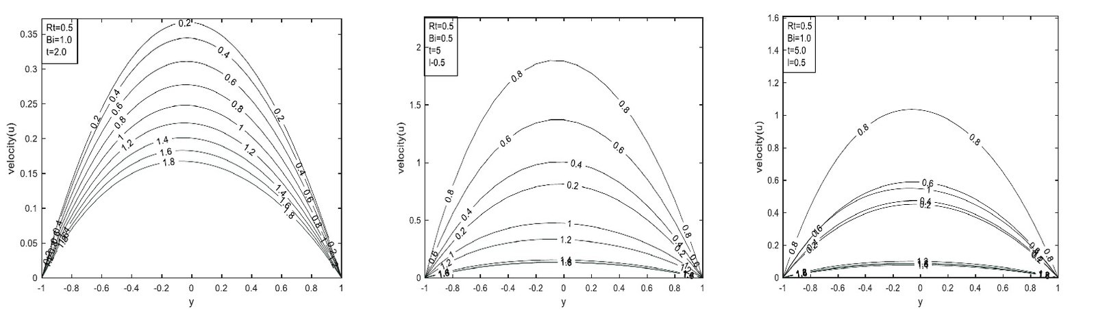
An increase in velocity is observed as the functional parameter increases, and notably, profiles from both fractional models converge as the parameter approaches one, indicating nearly identical behavior. Lower values indicate stronger memory or nonlocal effects that reduce flow velocity. As the parameter increases, memory effects weaken, allowing velocity to increase. When the parameter reaches one, the models revert to the classical case corresponding to standard Newtonian flow without memory, as shown in Figure 13.
Figure 14 shows the effect of buoyancy force Rt on skin friction. Across all models, skin friction decreases with increasing Rt, reflecting an inverse relationship: higher thermal radiation reduces momentum near the wall, lowering skin friction. The classical model exhibits a more rapid decrease in skin friction over time and reaches steady state faster than the fractional models. Since it does not account for memory effects, the classical model responds sharply and immediately to thermal radiation. The CF model introduces a non-singular memory kernel that moderates the rate of decrease in skin friction, producing a smoother and delayed response to time and Rt, indicating fluid memory of previous states. The ABC model, incorporating a strong nonlocal memory via a heavy-tailed kernel, yields the most subdued skin friction response, reflecting long-lasting memory effects and resulting in the lowest skin friction values among the three models.
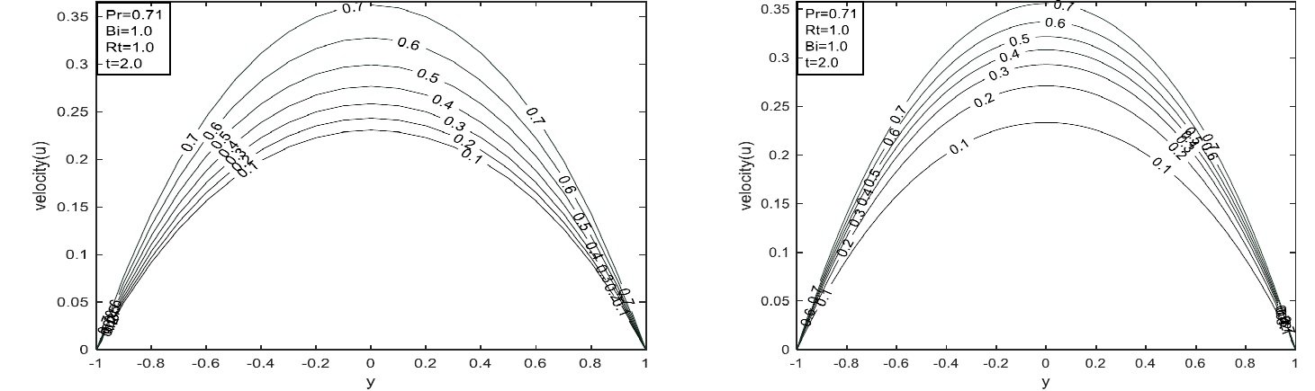
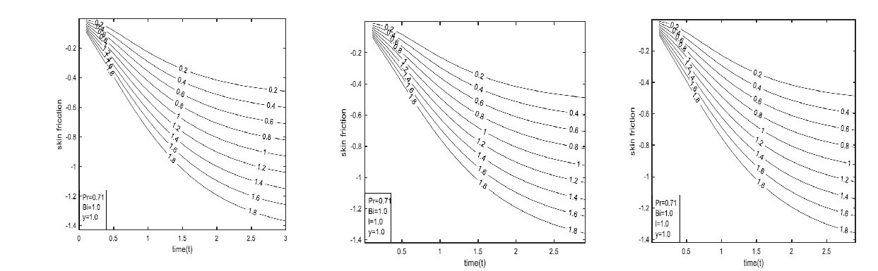
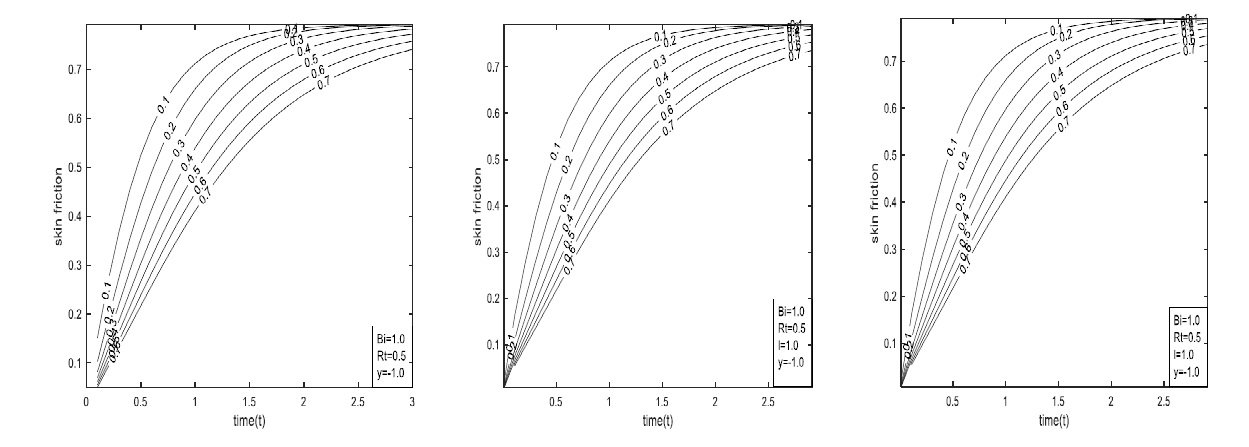
Figure 15 illustrates the effect of the Biot number on skin friction. An increase in Bi leads to increased skin friction at y = -1.0, whereas the opposite trend is observed at y = 1.0. The decrease in skin friction with rising Bi corresponds to enhanced thermal energy exchange with the surroundings, which thins the thermal boundary layer and reduces shear at the wall. The classical model assumes no memory effects, so skin friction changes immediately in response to thermal changes. The CF model, accounting for short-term memory via an exponential kernel, results in a smoother and more gradual friction response. The ABC model, with its nonlocal Mittag–Leffler kernel, introduces long-term memory effects that damp and delay the friction response further.
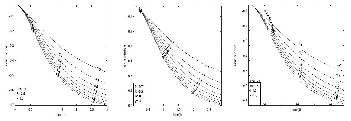
Figure 16 shows the effect of Pr on skin friction. Increasing Pr leads to a rise in opposing fluid velocity at y=-1, while the reverse is observed at y = 1. In all models, skin friction decreases as Pr increases, indicating that higher Prandtl numbers representing fluids with lower thermal diffusivity lead to weaker velocity gradients at the wall. The classical model shows a more rapid decline in skin friction, which stabilizes over time. The CF model smooth the transition, producing a more gradual decline compared to the classical case. The ABC model exhibits the most prolonged response, with skin friction decreasing slowly and stabilizing later, reflecting the stronger influence of past fluid behavior.
This study examined the influence of the buoyancy force parameter (Rt) and the Biot number (Bi) distribution parameter on transient natural convection flow within a vertical channel, incorporating fractional derivatives in the sense of Caputo–Fabrizio (CF) and Atangana–Baleanu–Caputo (ABC) models. The analytical solutions were found to be significantly affected by the buoyancy force parameter, Biot number, and Prandtl number (Pr). Based on the graphical and tabulated results, the following key conclusions are drawn:
For all models considered (Classical, CF, and ABC), the temperature, velocity, and volumetric flow rate increase with increasing buoyancy force parameter (Rt) and time (t).
In all models, skin friction decreases as the Prandtl number increases. This suggests that fluids with higher Pr indicating lower thermal diffusivity exhibit weaker velocity gradients near the wall.
The rate of heat transfer decreases with increasing Biot number (Bi) in all models, while it increases with the buoyancy force parameter (Rt).
Fluid velocity increases with higher values of Rt, Bi, and time in all models. However, skin friction exhibits a decreasing trend with respect to these parameters. Among the three models, the ABC model reaches the steady-state regime faster than the CF and Classical models.
These findings highlight the significance of fractional calculus in accurately capturing memory effects in transient natural convection and suggest that fractional models, particularly the ABC formulation, offer enhanced physical realism in modeling heat and fluid flow phenomena in porous and convective systems.
Numerical values for skin friction (\(\tau\)) and Nusselt number (\(Nu\)) of air (\(\Pr = 0.71\)) are presented in Table 1.
| \(Rt\) | \(t\) | \(\tau_{-1}\) | \(\tau_{1}\) | \(Nu_{-1}\) | \(Nu_{1}\) |
| -1 | 0.1 | 0.0499 | 0.0499 | -0.6806 | -0.6806 |
| 0.3 | 0.1190 | 0.1190 | -0.5506 | -0.5506 | |
| 0.5 | 0.1502 | 0.1502 | -0.5100 | -0.5100 | |
| 0.7 | 0.1615 | 0.1615 | -0.4968 | -0.4968 | |
| SS | 0.1667 | 0.1667 | -0.4987 | -0.4987 | |
| -0.7 | 0.1 | 0.0500 | 0.0350 | -0.6806 | -0.4764 |
| 0.3 | 0.1217 | 0.0806 | -0.5472 | -0.3888 | |
| 0.5 | 0.1633 | 0.0922 | -0.4973 | -0.3697 | |
| 0.7 | 0.1886 | 0.0859 | -0.4737 | -0.3708 | |
| SS | 0.2920 | -0.0065 | -0.4159 | -0.4239 | |
| -0.5 | 0.1 | 0.0500 | 0.0250 | -0.6806 | -0.3403 |
| 0.3 | 0.1235 | 0.0550 | -0.5450 | -0.2810 | |
| 0.5 | 0.1719 | 0.0534 | -0.4889 | -0.2762 | |
| 0.7 | 0.2066 | 0.0356 | -0.4583 | -0.2868 | |
| SS | 0.3745 | -0.1236 | -0.3622 | -0.3740 | |
| -0.3 | 0.1 | 0.0500 | 0.0500 | -0.6806 | -0.2042 |
| 0.3 | 0.1253 | 0.1253 | -0.5427 | -0.1731 | |
| 0.5 | 0.1806 | 0.1806 | -0.4804 | -0.1826 | |
| 0.7 | 0.2247 | 0.2247 | -0.4429 | -0.2029 | |
| SS | 0.4572 | 0.4592 | -0.3230 | -0.3190 | |
| -0.1 | 0.1 | 0.0500 | 0.0500 | -0.6806 | -0.0681 |
| 0.3 | 0.1271 | 0.0038 | -0.5404 | -0.0652 | |
| 0.5 | 0.1893 | -0.0240 | -0.4720 | -0.0891 | |
| 0.7 | 0.2428 | -0.0651 | -0.4275 | -0.1189 | |
| SS | 0.5416 | -0.3581 | -0.2748 | -0.2743 | |
| 0.3 | 0.1 | 0.0500 | -0.0150 | -0.2041 | 0.2041 |
| 0.3 | 0.1307 | -0.0474 | -0.1505 | 0.1505 | |
| 0.5 | 0.2153 | -0.1014 | -0.0980 | 0.0980 | |
| 0.7 | 0.2970 | -0.1658 | -0.0490 | 0.0490 | |
| SS | 0.7083 | -0.5917 | 0.1746 | -0.1746 | |
| 0.5 | 0.1 | 0.0500 | -0.0250 | -0.3403 | 0.3403 |
| 0.3 | 0.1325 | -0.0730 | -0.2584 | 0.2584 | |
| 0.5 | 0.2153 | -0.1402 | -0.1915 | 0.1915 | |
| 0.7 | 0.2970 | -0.2162 | -0.1330 | 0.1330 | |
| SS | 0.7914 | -0.7080 | 0.1247 | -0.1247 | |
| 0.7 | 0.1 | 0.0500 | -0.0350 | -0.4764 | 0.4764 |
| 0.3 | 0.1343 | -0.0986 | -0.3662 | 0.3662 | |
| 0.5 | 0.2240 | -0.1789 | -0.2851 | 0.2851 | |
| 0.7 | 0.3150 | -0.2666 | -0.2169 | 0.2169 | |
| SS | 0.8744 | -0.8750 | 0.0748 | -0.0748 | |
| 1.0 | 0.1 | 0.0500 | -0.0500 | -0.6805 | 0.6805 |
| 0.3 | 0.1370 | -0.1370 | -0.5280 | 0.5280 | |
| 0.5 | 0.2370 | -0.2370 | -0.4254 | 0.4254 | |
| 0.7 | 0.3421 | -0.3421 | -0.3429 | 0.3429 | |
| SS | 1.0001 | -1.0001 | -0.0006 | 0.0006 | |
| -1.0 | 0.1 | 0.0095 | 0.0095 | -0.8747 | -0.8747 |
| 0.3 | 0.0268 | 0.0268 | -0.7994 | -0.7994 | |
| 0.5 | 0.0424 | 0.0424 | -0.7533 | -0.7533 | |
| 0.7 | 0.0563 | 0.0563 | -0.7189 | -0.7189 | |
| SS | 0.1668 | 0.1668 | -0.5005 | -0.5005 | |
| -0.7 | 0.1 | 0.0569 | 0.0067 | -0.8748 | -0.6124 |
| 0.3 | 0.0268 | 0.0187 | -0.7994 | -0.5596 | |
| 0.5 | 0.0426 | 0.0295 | -0.7533 | -0.5273 | |
| 0.7 | 0.0569 | 0.0388 | -0.7189 | -0.5032 | |
| SS | 0.2909 | -0.0083 | -0.4247 | -0.4142 | |
| -0.5 | 0.1 | 0.0950 | 0.0048 | -0.8748 | -0.4374 |
| 0.3 | 0.0268 | 0.0134 | -0.7994 | -0.3997 | |
| 0.5 | 0.0427 | 0.0209 | -0.7533 | -0.3767 | |
| 0.7 | 0.0573 | 0.0271 | -0.7189 | -0.3594 | |
| SS | 0.3740 | -0.1247 | -0.3740 | -0.3740 | |
| -0.3 | 0.1 | 0.0095 | 0.0029 | -0.8748 | -0.2625 |
| 0.3 | 0.0269 | 0.0080 | -0.7994 | -0.2398 | |
| 0.5 | 0.0428 | 0.0123 | -0.7533 | -0.2260 | |
| 0.7 | 0.0578 | 0.0154 | -0.7189 | -0.2157 | |
| SS | 0.4572 | -0.2411 | -0.3242 | -0.3242 | |
| -0.1 | 0.1 | 0.0095 | 0.0010 | -0.8748 | -0.0875 |
| 0.3 | 0.0269 | 0.0026 | -0.7994 | -0.0799 | |
| 0.5 | 0.0430 | 0.0037 | -0.7533 | -0.0753 | |
| 0.7 | 0.0582 | 0.0037 | -0.7189 | -0.0719 | |
| SS | 0.5417 | -0.3576 | -0.2244 | -0.2244 | |
| 0.3 | 0.1 | 0.0095 | -0.0029 | -0.8748 | 0.2625 |
| 0.3 | 0.0269 | -0.0081 | -0.7994 | 0.2398 | |
| 0.5 | 0.0432 | -0.0136 | -0.7533 | 0.2260 | |
| 0.7 | 0.0590 | -0.0196 | -0.7189 | 0.2157 | |
| SS | 0.7079 | -0.5919 | -0.1746 | -0.1746 | |
| 0.5 | 0.1 | 0.0095 | -0.0048 | -0.8748 | 0.4374 |
| 0.3 | 0.0269 | -0.0135 | -0.7994 | 0.3997 | |
| 0.5 | 0.0434 | -0.0222 | -0.7533 | 0.3767 | |
| 0.7 | 0.0595 | -0.0313 | -0.7189 | 0.3594 | |
| SS | 0.7916 | -0.7079 | -0.1247 | -0.1247 | |
| 0.7 | 0.1 | 0.0095 | -0.0067 | -0.8748 | 0.6124 |
| 0.3 | 0.0269 | -0.0189 | -0.7994 | 0.5596 | |
| 0.5 | 0.0435 | -0.0308 | -0.7533 | 0.5273 | |
| 0.7 | 0.0599 | -0.0430 | -0.7189 | 0.5032 | |
| SS | 0.8749 | -0.8249 | -0.0748 | -0.0748 | |
| 1.0 | 0.1 | 0.0095 | -0.0095 | -0.8748 | 0.8747 |
| 0.3 | 0.0269 | -0.0269 | -0.7993 | 0.7993 | |
| 0.5 | 0.0437 | -0.0437 | -0.7533 | 0.7533 | |
| 0.7 | 0.0605 | -0.0605 | -0.7189 | 0.7189 | |
| SS | 1.0000 | -1.0000 | 0.0000 | 0.0000 |