
The wide-ranging applicability of the weighted Rayleigh (WR) distribution to different fields—such as medical sciences, engineering, agriculture, ecology, and finance—among others, and to different areas of research such as reliability and lifetime phenomena, has been documented in the existing literature. This implies that the Rayleigh distribution has been widely used because of the important role it plays in statistical modeling and operational research. However, the Modified Weighted Rayleigh (MWR) distribution is one of the special models obtained from the Modified Weighted Weibull (MWW) distribution [1]. Meanwhile, the MWR is a good distribution for fitting both real-life and simulation data. Numerous researchers, including [2– 6], have studied the MWW distribution.
The distribution function of the MWR distribution is given in (1) below: \[\begin{aligned} \label{eq1} G(x)=1-e^{-{\alpha{x^2}}{(1+\beta\gamma^2)}};\quad x,\alpha,\beta,\gamma>0, \end{aligned} \tag{1}\] where \(\alpha\) is a scale parameter and \(\beta\) and \(\gamma\) are shape parameters; the corresponding density function of (1) is given in (2): \[\begin{aligned} \label{eq2} g(x)=2\alpha(1+\beta\gamma^2)xe^{-{\alpha{x^2}}{(1+\beta\gamma^2)}};\quad x,\alpha,\beta,\gamma>0. \end{aligned} \tag{2}\]
Also, the survival and failure rate functions of the MWR distribution are, respectively, given by \[\begin{aligned} \label{eq3} \bar{G}(x)=1-\big(1-e^{-{\alpha{x^2}}{(1+\beta\gamma^2)}}\big)=e^{-{\alpha{x^2}}{(1+\beta\gamma^2)}};\quad x,\alpha,\beta,\gamma>0. \end{aligned} \tag{3}\] and \[\begin{aligned} \label{eq4} Fal(x)=\dfrac{2\alpha(1+\beta\gamma^2)xe^{-{\alpha{x^2}}{(1+\beta\gamma^2)}}}{1-\big(1-e^{-{\alpha{x^2}}{(1+\beta\gamma^2)}}\big)}. \end{aligned} \tag{4}\]
These expressions can be found in [1].
Topp-Leone distribution has indeed gained much ground, as evidenced by the presence of several different distributions in the literature by several researchers such as [7– 16], etc. Most of them applied their work to different real-life data, while some conducted simulation studies in their research.
Work on the Topp-Leone (TL) family of distributions has been carried out by [7, 17, 18]. The CDF and the associated PDF, survival, and failure-rate functions are given by (5)–(8), respectively, below: \[ F_{TL\text{-}CDF}(x) ={[G(x)]^\lambda}{[2-G(x)]^\lambda}={[1-(\bar{G}(x))^2]^\lambda};\; x\epsilon\Re,\ \theta>0, \ \tag{5}\] \[\label{eq6} f_{TL\text{-}PDF}(x) =2\lambda\,g(x)\,\bar{G}(x)\,[1-(\bar{G}(x))^2]^{\lambda-1};\ \ \theta>0, \ \tag{6}\] \[\label{eq7} \bar{F}_{TL\text{-}Rel}(x) =1-[1-(\bar{G}(x))^2]^\lambda, \tag{7}\] and \[\begin{aligned} \label{eq8} Fal_{TL}(x)=\dfrac{2\lambda\,g(x)\,\bar{G}(x)\,[1-(\bar{G}(x))^2]^{\lambda-1}}{1-[1-(\bar{G}(x))^2]^\lambda}, \end{aligned} \tag{8}\] where \(g(t)=G^\prime(x)\) and \(\bar{G}(x)=1-G(x)\).
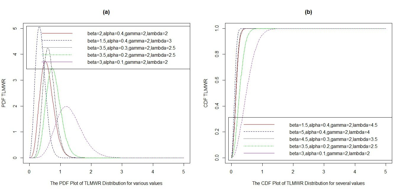
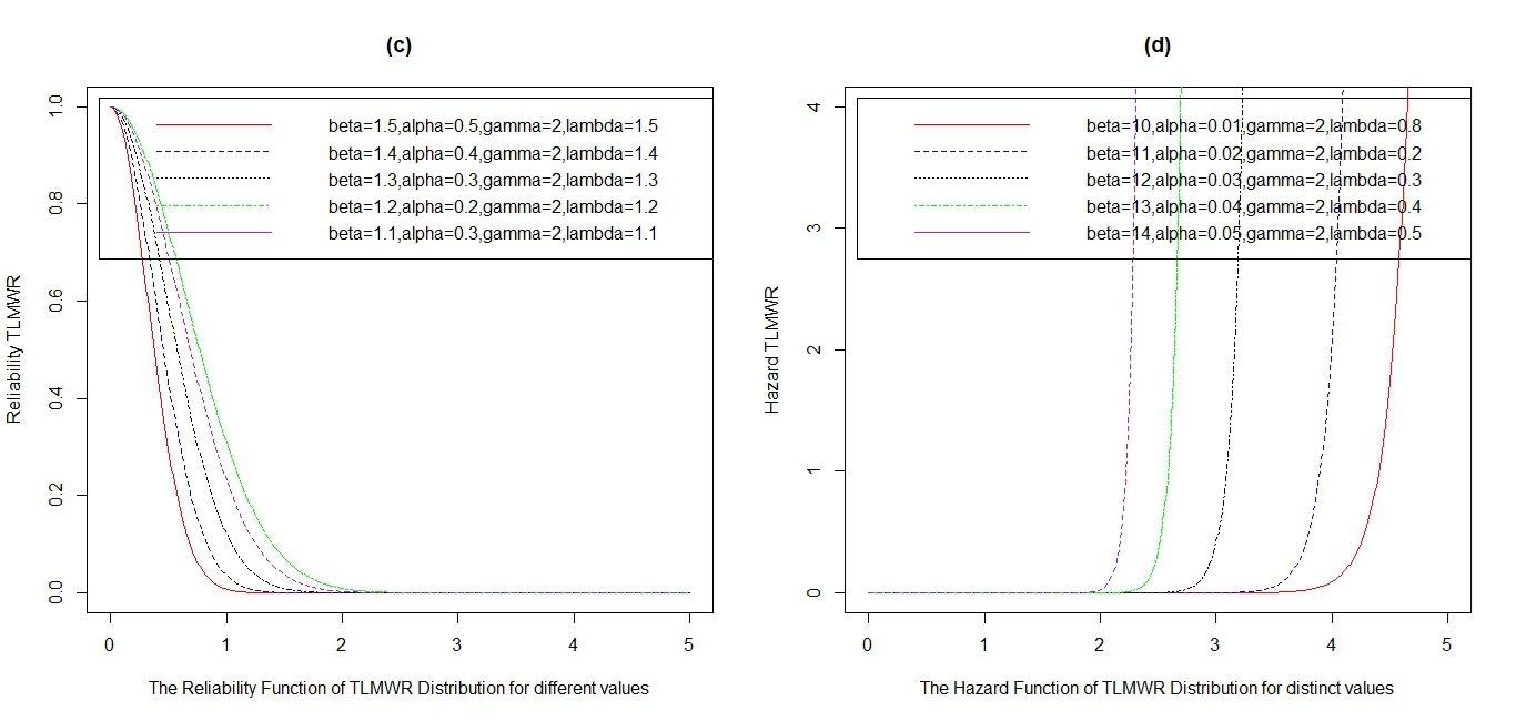
Here, the Topp-Leone Modified Weighted Rayleigh (TLMWR) distribution is obtained because it is very useful for modeling unimodal and real-life data sets with an asymmetric nature. Also, it is better to use the proposed distribution in the case of large, right-skewed data sets. Basically, its advantage is due to its flexible nature without the Weibull distribution and its capability to handle real-life phenomena arising from medicine, engineering, and physical sciences [8, 19]. Hence, the plot of the distribution is right-skewed, and \((\gamma=2)\) is constant as the value of the scale parameter, while the values of the other parameters \(\alpha\), \(\beta\), and \(\lambda\) decrease. There is an inward shift at the starting point in Figure 1 as a decrease occurs in the peak of the curve. Also, its survival plot has an L-shape, as the value of \(\gamma\) is constant at \((\gamma=2)\) and the values of \(\alpha\), \(\beta\), and \(\lambda\) vary (decrease), while the failure rate has a J-shape and experiences an inward shift toward the left as the other parameters decrease in Figure 2.
The paper is arranged as follows: In §2, the TLMWR distribution and its properties are discussed. The moments and generating function appear in §3, and the order statistics of the TLMWR distribution are described in §4. Then, the maximum likelihood estimation method is used to obtain the model parameter estimates in §5. We carry out model validation of some models considered in the study with two different illustrations in §6. Lastly, §7 presents the discussion, results, and concluding remarks.
This study obtains both the distribution and density functions of the TLMWR by substituting Eq. (3) into (5), which gives: \[\begin{aligned} \label{eq9} F_{TLMWR}(x)=\left[1-\left(e^{-\alpha(1+\beta\gamma^2)x^2}\right)^2\right]^{\lambda}, \qquad \lambda \ge 0. \end{aligned} \tag{9}\]
Differentiating (9) yields the corresponding density function as \[\begin{aligned} \label{eq10} f_{TLMWR}(x)=2\lambda\,\bigl(2\alpha(1+\beta\gamma^2)x\bigr)\,e^{-2\alpha(1+\beta\gamma^2)x^2}\,\left[1-e^{-2\alpha(1+\beta\gamma^2)x^2}\right]^{\lambda-1}, \qquad \alpha,\beta,\gamma,\lambda>0,\ x\ge 0, \end{aligned} \tag{10}\] where \(\alpha\), \(\beta\), and \(\lambda\) are shape parameters, and \(\gamma\) is a scale parameter. Now, if a random variable \(X\) has density function \(f_{TLMWR}(x)\) in Eq. (10) above, it can be written as \(X\sim\text{TLMWR}(\alpha,\beta,\gamma,\lambda)\). Also, the PDF and CDF plots for TLMWR are depicted in Figure 1.
Remark 1. From the TLMWR distribution in Eq. (10), some well-known and new distributions in the literature arise as special cases when one or more parameters equal 1. These are:
When \(\beta=1\), Eq. (10) becomes the Topp–Leone Modified Exponential Rayleigh (TLMER) distribution.
If \(\alpha=1\), Eq. (10) turns into the Topp–Leone Modified Weibull model [18].
For \(\lambda=1\), Eq. (10) reduces to the MWR distribution [1].
When \(\theta=\beta=1\), Eq. (10) gives the Modified Weighted Exponential (MWE) distribution [1].
When \(\beta=\gamma=0\), Eq. (10) leads to the Topp–Leone Exponential distribution as in [13].
If \(\lambda=\alpha=1\), Eq. (10) yields the Weighted Rayleigh (WR) distribution.
For \(\beta=0\), Eq. (10) becomes a weighted distribution.
The survival function of the TLMWR distribution can be obtained from (7) as \[\begin{aligned} \label{eq11} \bar{F}_{TLMWR}(x)=1-\left[1-e^{-2\alpha(1+\beta\gamma^2)x^2}\right]^{\lambda}. \end{aligned} \tag{11}\]
Let \(w=2\alpha(1+\beta\gamma^2)\). The failure rate function is obtained from (8) as \[\begin{aligned} \label{eq12} Fal_{TLMWR}(x)=\frac{f_{TLMWR}(x)}{\bar{F}_{TLMWR}(x)}=\frac{2\lambda\,w x\,e^{-w x^2}\,\left[1-e^{-w x^2}\right]^{\lambda-1}}{1-\left(1-e^{-w x^2}\right)^{\lambda}}, \end{aligned} \tag{12}\] while the cumulative failure (CFal) of the TLMWR distribution is given by \[\begin{aligned} CFal_{TLMWR}(x)=-\log\left[1-\left(1-e^{-2\alpha x^{2}(1+\beta\gamma^{2})}\right)^{\lambda}\right]. \end{aligned}\]
Moreover, the survival and failure rate plots of the TLMWR distribution are depicted in Figure 2.
The density, distribution, and failure rate functions of the proposed distribution are examined as \(x\) tends to zero and infinity (\(0\) and \(\infty\)). Thus, \(\lim_{x\rightarrow 0} f_{TLMWR}(x)\) and \(\lim_{x\rightarrow \infty} f_{TLMWR}(x)\) are given as follows: \[\begin{aligned} \lim_{x\rightarrow 0} f_{TLMWR}(x) &=\lim_{x\rightarrow 0}\left[2\lambda\,w x\,e^{-w x^{2}}\left(1-e^{-w x^{2}}\right)^{\lambda-1}\right]=0,\\ \lim_{x\rightarrow \infty} f_{TLMWR}(x) &=\lim_{x\rightarrow \infty}\left[2\lambda\,w x\,e^{-w x^{2}}\left(1-e^{-w x^{2}}\right)^{\lambda-1}\right]=0. \end{aligned}\]
Note that both limits above are \(0\) as \(x\rightarrow 0\) and as \(x\rightarrow \infty\). This shows that the TLMWR distribution has a unique mode (i.e., it is unimodal; see Figure 1, plot (a)) [20, 21]. The distribution and failure rate behaviour are obtained below: \[\begin{aligned} \lim_{x\rightarrow 0} Fal_{TLMWR}(x)&=\lim_{x\rightarrow 0}\left[1-e^{-w x^{2}}\right]^{\lambda}=0,\\ \lim_{x\rightarrow \infty} Fal_{TLMWR}(x)&=\lim_{x\rightarrow \infty}\left[1-e^{(w x^{2})}\right]^{\lambda}=1,\\ \lim_{x\rightarrow 0} Fal_{TLMWR}(x)&=\lim_{x\rightarrow 0}\left[\dfrac{2\lambda\,w x\,e^{-w x^{2}}\left(1-e^{-w x^{2}}\right)^{\lambda-1}}{1-\left(1-e^{-w x^{2}}\right)^{\lambda}}\right]=0,\\ \lim_{x\rightarrow \infty} Fal_{TLMWR}(x)&=\lim_{x\rightarrow \infty}\left[\dfrac{2\lambda\,w x\,e^{-w x^{2}}\left(1-e^{-w x^{2}}\right)^{\lambda-1}}{1-\left(1-e^{-w x^{2}}\right)^{\lambda}}\right]=0. \end{aligned}\]
Following the series representation by Prudnikov et al. [22] and used by [7], the cumulative distribution and density can be written in the form of the exponentiated-G model as \[\begin{aligned} (1+x)^{\alpha}=\sum\limits_{j=0}^{\infty}(-1)^j\dfrac{\Gamma(\alpha+1)}{j!(\alpha+1-j)}x_j, \end{aligned}\] Thus, the CDF of the TLMWR distribution can be expressed as \[\begin{aligned} F_{TLMWR}(x)=\sum\limits_{j=0}^\infty(-1)^j\dfrac{\Gamma(\lambda+1)}{j!(\lambda+1-j)}\left(e^{-w{x^2}}\right)^2j, \end{aligned}\] and its associated density can also be written as \[\begin{aligned} \label{eq13} f_{TLMWR}(x)=\sum\limits_{j=0}^\infty(-1)^j\dfrac{2\Gamma(\lambda+1)}{j!(\lambda+1-j)}(wx)\times\left(e^{-w{x^2}}\right)^{(j+1)}. \end{aligned} \tag{13}\]
The QF of the TLMWR distribution is expressed as \(Q_{TLMWR}(u)=F^{-1}(u)\). Suppose \(F_{TLMWR}(u)=u\in(0,1)\) for \(x\): \[\begin{aligned} \left(1-e^{-w x^{2}}\right)^{\lambda}=u \;\Rightarrow\; 1-e^{-w x^{2}}=u^{\frac{1}{\lambda}} \;\Rightarrow\; e^{-w}=1-u^{\frac{1}{\lambda}}. \end{aligned}\]
Then, \[\begin{aligned} Q_{TLMWR}(u)=F^{-1}(u)=\sqrt{-\frac{1}{w}\,ln\!\left(1-\left(e^{-w x^{2}}\right)^{\frac{1}{\lambda}}\right)}. \end{aligned}\]
For example, when \(\alpha=1.5\), \(\beta=1\), \(\gamma=1.5\), and \(\lambda=2.5\).
Setting \(F_{TLMWR}(x)=u\), where \(u\) is a probability such as \(0.25\), \(0.50\), or \(0.75\), \[u=(1-e^{-w x^{2}})^{\lambda}, \quad \text{recall} \quad w=2\alpha(1+\beta\gamma^{2}).\]
Taking the \(\lambda\)-th root, \(u^{\frac{1}{\lambda}}=1-e^{-w x^{2}}\), \(x^{2}=\frac{1}{w}ln(1-u^{\frac{1}{\lambda}})\). So, the quantile is \[\begin{aligned} Q_{TLMWR}(u)=\sqrt{-\dfrac{1}{w}ln(1-u^{\frac{1}{\lambda}})}, \end{aligned}\] where \(w=2\alpha(1+\beta\gamma^{2})=2\times1.5\,(1+1\times(2.5)^{2})=9.\)
By estimating the first, second, and third quantiles of the TLMWR distribution, we get
\(\bullet\ \text{for the 1st quantile } Q_{TLMWR}(0.25)\) \[Q_{TLMWR}(0.25)=\sqrt{-\frac{1}{9}\,ln\!\left(1-(0.25)^{\frac{1}{2.5}}\right)}=0.3586.\]
\(\bullet\ \text{for the median quantile } Q_{TLMWR}(0.5)\) \[Q_{TLMWR}(0.5)=\sqrt{-\frac{1}{9}\,ln\!\left(1-(0.5)^{\frac{1}{2.5}}\right)}=0.4720.\]
\(\bullet\ \text{for the third quantile } Q_{TLMWR}(0.5)\) \[Q_{TLMWR}(0.75)=\sqrt{-\frac{1}{9}\,ln\!\left(1-(0.75)^{\frac{1}{2.5}}\right)}=0.6009.\]
Meanwhile, setting \(u=\frac{1}{2}\) in \(Q_{TLMWR}(u)\), the equation becomes the median of the TLMWR distribution. By applying Bowley’s measure and Moors’ coefficients of skewness (Sk) and kurtosis (Kt) [23, 24], as used in [25], they are given as \[\begin{aligned} Sk=\dfrac{Q(0.25)+Q(0.75)-2Q(0.5)}{Q(0.75)-Q(0.25)}, \end{aligned}\] and \[\begin{aligned} Kt=\dfrac{Q(0.875)-Q(0.625)+Q(0.375)-Q(0.125)}{Q(0.75)-Q(0.25)}. \end{aligned}\]
Furthermore, we compute the median, Sk, and Kt of the distribution (using the QF) for several values of \(\lambda\), \(\alpha\), \(\beta\), and \(\gamma\), and present them in Table 1 below. It can be noted from Table 1 that, for fixed \(\alpha\), \(\beta\), and \(\gamma\) with increasing values of \(\lambda\), only the skewness increases, while the other two decrease as the values of \(\lambda\) increase.
| Parameters | Quantiles | |||||
|---|---|---|---|---|---|---|
| \(\lambda\) | \(\alpha\) | \(\beta\) | \(\gamma\) | Median | Sk | Kt |
| 0.70 | 0.06 | 0.05 | 1.50 | 7.8954 | -1.4738 | 2.7941 |
| 1.00 | 6.6607 | -1.1652 | 2.3311 | |||
| 2.00 | 4.3951 | -0.5988 | 1.4815 | |||
| 5.00 | 1.8915 | 0.0271 | 0.5426 | |||
| 0.70 | 0.09 | 0.07 | 2.00 | 4.5748 | -0.6437 | 1.5489 |
| 1.00 | 3.8594 | -0.41649 | 1.2806 | |||
| 2.00 | 2.5467 | -0.1367 | 0.7883 | |||
| 5.00 | 1.0960 | 0.2260 | 0.2443 |
The general r-th moment follows from a derivation using the binomial (generalized) expansion for \((1-y)^{\lambda-1}\) with \(y=e^{-w x^{2}}\) [7]. \[\begin{aligned} (1-e^{-w x^{2}})^{\lambda-1} =\sum\limits_{j=0}^{\infty}\begin{pmatrix}\lambda-1 \\ j \end{pmatrix}(-1)^{j}e^{-j w x^{2}} , \end{aligned}\] Then, \[\begin{aligned} f_{TLMWR}(x)=2\lambda w x\sum\limits_{j=0}^{\infty}\begin{pmatrix}\lambda-1 \\ j\end{pmatrix}(-1)^{j}e^{-(j+1)w x^{2}}, \end{aligned}\] where \(2\lambda(1+\beta\gamma^{2})=w\). Hence, for the r-th raw moment of the proposed distribution, we have \[\begin{aligned} E[X^{r}]=\int_{0}^{\infty}x^{r}f_{TLMWR}(x)\,dx =2\lambda w\sum\limits_{j=0}^{\infty}\begin{pmatrix}\lambda-1 \\ j\end{pmatrix}\int_{0}^{\infty}x^{r+1}e^{-(j+1)w x^{2}}\,dx. \end{aligned}\]
Use the integral for \(a>0\), \(m>0\): \[\begin{aligned} \int_{0}^{\infty}x^{a}e^{-m x^{2}}\,dx=\dfrac{1}{2}m^{-\frac{a+1}{2}}\Gamma\!\left(\frac{a+1}{2}\right). \end{aligned}\]
Take \(a=r+1\) and \(m=(j+1)w\). Thus, \[\begin{aligned} \int_{0}^{\infty}x^{r+1}e^{-(j+1)w x^{2}}\,dx =\dfrac{1}{2}\bigl((j+1)w\bigr)^{-\frac{r+2}{2}}\Gamma\!\left(\dfrac{r+2}{2}\right). \end{aligned}\]
Hence we get \[\begin{aligned} E[X^{r}] =\lambda w^{-\frac{r}{2}}\Gamma\!\left(\dfrac{r+2}{2}\right) \sum\limits_{j=0}^{\infty}(-1)^{j}\begin{pmatrix}\lambda-1 \\ j \end{pmatrix}(j+1)^{-\frac{r+2}{2}}, \end{aligned}\] and letting \[S_{r}(\lambda)=\sum\limits_{j=0}^{\infty}(-1)^{j}\begin{pmatrix}\lambda-1\\ j \end{pmatrix}(j+1)^{-\frac{r+2}{2}}, \quad r \ge 2.\]
Therefore, the general raw moment for the TLMWR distribution is \[\begin{aligned} E(X^{r})=\lambda w^{-\frac{r}{2}}\Gamma\!\left(\dfrac{r+2}{2}\right)S_{r}(\lambda), \end{aligned} \tag{14}\] for the orders we need explicitly: \[\begin{aligned} r=&\,1,\quad E[X]=\lambda w^{-\frac{1}{2}}\Gamma\!\left(\dfrac{3}{2}\right)S_{1} =\lambda w^{-\frac{1}{2}}\dfrac{\sqrt{\pi}}{2}S_{1},\\ r=&\,2,\quad E[X^{2}]=\lambda w^{-1}\Gamma(2)S_{2}=\lambda w^{-1}S_{2},\\ r=&\,3,\quad E[X^{3}]=\lambda w^{-\frac{3}{2}}\Gamma\!\left(\dfrac{5}{2}\right)S_{3} =\lambda w^{-\frac{3}{2}}\dfrac{3\sqrt{\pi}}{4}S_{3},\\ r=&\,4,\quad E[X^{4}]=\lambda w^{-2}\Gamma(3)S_{4}=\lambda w^{-2}\cdot 2\,S_{4}. \end{aligned}\]
Let \(\mu=E[X]\) and \(\mu_{r}^{\prime}=E[X^{r}]\). Also, the variance is \(\mu_{2}=\mathrm{Var}(X)=\mu_{2}^{\prime}-\mu^{2}\).
The 3rd central moment: \[\begin{aligned} \mu_{3}=E[(X-\mu)^{3}]=\mu_{3}^{\prime}-3\mu\,\mu_{2}^{\prime}+2\mu^{3}. \end{aligned}\]
The 4th central moment: \[\begin{aligned} \mu_{4}=E[(X-\mu)^{4}]=\mu_{4}^{\prime}-4\mu\,\mu_{3}^{\prime}+6\mu^{2}\mu_{2}^{\prime}+3\mu^{4}. \end{aligned}\]
Substitute the closed-form raw moments above to obtain explicit series expressions for the coefficient of variation, skewness, and (excess) kurtosis: \[\begin{aligned} CoV_{TLMWR}=\dfrac{\mu_{2}}{\mu_{1}}-1=\sqrt{\dfrac{\mu_{2}^{\prime}-(\mu_{1}^{\prime})^{2}}{\mu_{1}}}-1, \end{aligned}\] \[\begin{aligned} Sk_{TLMWR}=\dfrac{\mu_{3}}{(\mu_{2})^{3/2}}=\dfrac{\mu_{3}^{\prime}-3\mu\,\mu_{2}^{\prime}+2\mu^{3}}{(\mu_{2}^{\prime}-\mu^{2})^{3/2}}, \end{aligned}\] and \[\begin{aligned} Kt_{TLMWR}=\dfrac{\mu_{4}}{(\mu_{2})^{2}}=\dfrac{\mu_{4}^{\prime}-4\mu\,\mu_{3}^{\prime}+6\mu^{2}\mu_{2}^{\prime}+3\mu^{4}}{(\mu_{2}^{\prime}-\mu^{2})^{2}}-3. \end{aligned}\]
Each \(\mu_{r}^{\prime}\) is substituted from the series expressions above (with the general factor).
Table 2 contains the computed 1st to 4th moments, variance, and coefficients of skewness and kurtosis. It is observed that the TLMWR distribution can be positively/right-skewed for \((Sk>0)\). At the same time, it is platykurtic for \((Kt<3)\) and mesokurtic \((Kt\approx 0)\), respectively, for some fixed values of the parameters and several values of a parameter [13, 18].
| \(\mu_{S}^{\prime}\) | \(\lambda,\ \alpha,\ \beta,\ \gamma\) | \(\lambda,\ \alpha,\ \beta,\ \gamma\) | \(\lambda,\ \alpha,\ \beta,\ \gamma\) | \(\lambda,\ \alpha,\ \beta,\ \gamma\) |
|---|---|---|---|---|
| \(\mu_{1}^{\prime}\) | 0.0215 | 0.0755 | 0.1510 | 0.2614 |
| \(\mu_{2}^{\prime}\) | 0.0055 | 0.0218 | 0.0436 | 0.9062 |
| \(\mu_{3}^{\prime}\) | 0.0016 | 0.0074 | 0.0148 | 0.0341 |
| \(\mu_{4}^{\prime}\) | 0.0005 | 0.0028 | 0.0057 | 1.8915 |
| \(\sigma^{2}\) | 0.0050 | 0.0161 | 0.0208 | 0.8379 |
| \(CS_{K}\) | 0.2723 | 0.2308 | 0.4617 | 2.7701 |
| \(CK_{T}\) | 0.1814 | 0.1538 | 0.3076 | 1.8285 |
This study uses the probability density function (PDF) of the TLMWR distribution and expands the factor \((1-e^{-w x^{2}})^{\lambda-1}\) by the generalized binomial series: \[\begin{aligned} (1-e^{-w x^{2}})^{\lambda-1} =\sum_{j=0}^{\infty}\begin{pmatrix}\lambda-1 \\ j\end{pmatrix}(-1)^{j}e^{-j w x^{2}}. \end{aligned}\]
Suppose \(X \sim \mathrm{TLMWR}(\alpha,\beta,\lambda,\gamma)\). Then the MGF of \(X\) is denoted by \(M_{X}(t)\) and defined by \[\begin{aligned} M_{TLMWR}(t) =\int_{0}^{\infty} e^{t x} f_{TLMWR}(x)\,dx =\int_{0}^{\infty} e^{t x}\,2\lambda w x\,e^{-w x^{2}}(1-e^{-w x^{2}})^{\lambda-1}\,dx, \end{aligned}\] \[\begin{aligned} \label{eq15} M_{TLMWR}(t) =2\lambda w \sum_{j=0}^{\infty}\begin{pmatrix}\lambda-1 \\ j\end{pmatrix}(-1)^{j} \int_{0}^{\infty} x\,e^{t x-(j+1)w x^{2}}\,dx . \end{aligned} \tag{15}\]
The remaining integral is elementary after completing the square. For \(b>0\) and \(c\in\mathbb{R}\), \[\begin{aligned} I(b,c)=\int_{0}^{\infty} x\,e^{-b x^{2}+c x}\,dx =\frac{1}{2b}+\frac{c\sqrt{\pi}}{4 b^{3/2}}\,\exp\!\left(\frac{c^{2}}{4b}\right)\operatorname{erfc}\!\left(-\frac{c}{2\sqrt{b}}\right), \end{aligned}\] which can be obtained by completing the square and using Gaussian integral identities [25, 26].
Set \(b=(j+1)w\) and \(c=t\). Substituting into the expression gives the series form for the MGF: \[\begin{aligned} M_{TLMWR}(t) =2\lambda w \sum_{j=0}^{\infty}\begin{pmatrix}\lambda-1 \\ j\end{pmatrix}(-1)^{j} \left[ \frac{1}{2(j+1)w} +\frac{t\sqrt{\pi}}{4\big((j+1)w\big)^{3/2}} \exp\!\left(\frac{t^{2}}{4(j+1)w}\right) \operatorname{erfc}\!\left(-\frac{t}{2\sqrt{(j+1)w}}\right) \right], \end{aligned}\] \[\begin{aligned} \label{eq16} M_{TLMWR}(t) &=\lambda \sum_{j=0}^{\infty}\begin{pmatrix}\lambda-1 \\ j\end{pmatrix}(-1)^{j}\frac{1}{j+1} +\lambda \sum_{j=0}^{\infty}\begin{pmatrix}\lambda-1 \\ j\end{pmatrix}(-1)^{j} \frac{t\sqrt{\pi}}{2(j+1)^{3/2} w^{1/2}} \notag\\ &\quad\times \exp\!\left(\frac{t^{2}}{4(j+1)w}\right) \operatorname{erfc}\!\left(-\frac{t}{2\sqrt{(j+1)w}}\right). \end{aligned} \tag{16}\]
See Cordeiro et al. [27] and Al-Omari and Dobbah [28]. Eq. (16) is the moment generating function of the TLMWR distribution.
In the statistical sciences, order statistics are an important concept with a wide range of applicability in modeling. Suppose a random i.i.d. sample \(\{X_1, X_2, \ldots, X_n\}\) from the TLMWR distribution; then the density function of the \(k\)-th order statistic \(OS_{TLMWR\_(i)}\) is given by the standard formula \[\begin{aligned} \label{eq17} OS_{TLMWR\_(i)}(x)=\dfrac{n!}{(k-1)!(n-k)!}\left[F_{TLMWR}(x)\right]^{k-1} \left[1-F_{TLMWR}(x)\right]^{n-k}f_{TLMWR}(x), \quad x \geq 0 . \end{aligned} \tag{17}\] Inserting both the CDF and PDF of the TLMWR defined in (9) and (10), respectively, into (17), we get \[\begin{aligned} \label{eq18} OS_{TLMWR}(x)=\dfrac{n!}{(k-1)!(n-k)!}\left(1-e^{-w x^2}\right)^{\lambda(k-1)}\left[1-\left(1-e^{-w x^2}\right)^{\lambda}\right]^{n-k} 2\lambda w x e^{-w x^2}\left(1-e^{-w x^2}\right)^{\lambda-1}, \end{aligned} \tag{18}\] where \(w=2\alpha(1+\beta\gamma^{2})\).
We further show the algebraic simplifications for two cases, \(k=1\) (minimum) and \(k=n\) (maximum), and give the CDFs and simplified PDFs. Thus, using the general \(k\)-th order statistic PDF of the TLMWR distribution in (18) and letting \(k=1\) in the combinatorial factor, we have \[\dfrac{n!}{(1-1)!(n-1)!}=\dfrac{n!}{0!(n-1)!}=n.\] Then, \(\left[F_{TLMWR}(x)\right]^{k-1}=\left[F_{TLMWR}(x)\right]^0=1\). The TLMWR PDF becomes \[\begin{aligned} f_{TLMWR(1:n)}(x)= n\left[F_{TLMWR}(x)\right]^{n-1}f_{TLMWR}(x). \end{aligned}\] Substituting both the PDF and CDF of the TLMWR distribution into the above equation, we obtain \[\begin{aligned} f_{TLMWR(1:n)}(x)=2n\lambda w x e^{w x^2}\left(1-e^{w x^2}\right)^{\lambda-1}\left[1-\left(1-e^{w x^2}\right)^{\lambda}\right]^{n-1}. \end{aligned}\] Also, the CDF for \(k=1\) is given as \[\begin{aligned} F_{TLMWR(1:n)}(x)=P(X_{1:n} \leq x)=1-\left[1-\left(1-e^{w x^2}\right)^{\lambda}\right]^{n}. \end{aligned}\]
Furthermore, when \(k=n\) (the maximum), the combinatorial factor is \(\dfrac{n!}{(n-1)!0!}=n\) and \(\left[1-F_{TLMWR}(x)\right]^0=1\). Thus, \[\begin{aligned} F_{TLMWR(n:n)}(x)= n\left[F_{TLMWR}(x)\right]^{n-1}f_{TLMWR}(x). \end{aligned}\] Likewise, putting the PDF and CDF of the TLMWR distribution into the equation, we get \[\begin{aligned} F_{TLMWR(1:n)}(x)=2n\lambda w x e^{w x^2}\left(1-e^{w x^2}\right)^{\lambda(n-1)}\left(1-e^{w x^2}\right)^{\lambda-1}. \end{aligned}\] Also, combining the power of \(\left(1-e^{w x^2}\right)\) becomes \[\begin{aligned} F_{TLMWR(1:n)}(x)=2n\lambda w x e^{w x^2}\left(1-e^{w x^2}\right)^{\lambda n-1}. \end{aligned}\] The CDF of the maximum is [7, 13] \[\begin{aligned} F_{TLMWR(n:n)}(x)=P(X_{n:n} \leq x)=\left(1-e^{w x^2}\right)^{\lambda n}. \end{aligned}\]
Here, we discuss the method of parameter estimation for the TLMWR distribution. Suppose \(x_1, x_2, \ldots, x_n\) are a random sample of size \(n\) from the TLMWR distribution. Then, the log-likelihood (LL) function is given by \[\begin{aligned} \label{eq19} LL_{TLMWR}(x, \alpha, \beta, \gamma, \lambda) &=\sum_{i=1}^{n} f_{TLMWR}(x_i) \notag\\ &= n\log 2 + n\log \lambda + n\log w + \sum_{i=1}^{n}\log x_{i} – w\sum_{i=1}^{n} x_{i}^{2} + (\lambda-1)\sum_{i=1}^{n}\log\!\left(1-e^{-w x_{i}^{2}}\right). \end{aligned} \tag{19}\]
By differentiating (19), we can obtain the parameters by solving the nonlinear equations, namely \[V(\varphi)=\left(\frac{\partial LL}{\partial \lambda}, \frac{\partial LL}{\partial \alpha}, \frac{\partial LL}{\partial \beta}, \frac{\partial LL}{\partial \gamma}\right)^{\!T} =(V_{\lambda}, V_{\alpha}, V_{\beta}, V_{\gamma})^{T} [18,25],\] given as follows: \[ V_{\lambda} =\frac{n}{\lambda}+\sum_{i=1}^{n}\log\!\left(1-e^{w x_{i}^{2}}\right), \label{eq20}\ \tag{20}\] \[V_{\alpha} =\left(\frac{n}{w}-\sum_{i=1}^{n} x_{i}^{2} + (\lambda-1)\sum_{i=1}^{n}\frac{x_{i}^{2} e^{-w x_{i}^{2}}}{1-e^{-w x_{i}^{2}}}\right) 2(1+\beta\gamma^{2}),\ \tag{21}\] \[V_{\beta} =\left(\frac{n}{w}-\sum_{i=1}^{n} x_{i}^{2} + (\lambda-1)\sum_{i=1}^{n}\frac{x_{i}^{2} e^{w x_{i}^{2}}}{1-e^{-w x_{i}^{2}}}\right) 2\alpha\gamma^{2},\ \tag{22}\] \[V_{\gamma} =\left(\frac{n}{w}-\sum_{i=1}^{n} x_{i}^{2} + (\lambda-1)\sum_{i=1}^{n}\frac{x_{i}^{2} e^{-w x_{i}^{2}}}{1-e^{-w x_{i}^{2}}}\right) 4\alpha\beta\gamma. \label{eq23} \tag{23}\]
The values of the parameters \(\lambda\), \(\alpha\), \(\beta\), and \(\gamma\) in Eqs. (20)–(23) are difficult to estimate because the likelihood equation is complex. However, we use R and Python software to estimate the parameters.
This study checks each parameter to determine its mathematically valid range.
\(\bullet\ \alpha{:}\quad\) appears inside \(\log\!\bigl(2\alpha(1+\beta\gamma^{2})\bigr)\) and as a multiplier, and must satisfy \(\alpha>0\).
\(\bullet\ \beta{:}\quad\) appears inside \((1+\beta\gamma^{2})\), which is required to be \(1+\beta\gamma^{2}>0\) for the \(\log\) argument to be positive. This means \(\beta>-\dfrac{1}{\gamma}\) if \(\gamma\neq 0\).
\(\bullet\ \gamma{:}\quad\) free real number (since it appears squared). Domain: \(\gamma\in\mathbb{R}\).
\(\bullet\ \lambda{:}\quad\) appears inside \(\log(\lambda)\) and must satisfy \(\lambda>0\).
Other parts with examples are in the appendix.
A Monte Carlo (MC) simulation study is carried out to investigate the asymptotic behaviour of the MLE and to compute: \[\begin{aligned} \text{Average Bias (ABias)}\; &= \;\frac{1}{n}\sum_{i=1}^{n}\left(\hat{\theta}_i-\theta_0\right),\\ \text{Mean Square Error (MSE)} \; &= \;\frac{1}{n}\sum_{i=1}^{n}\left(\hat{\theta}_i-\theta_0\right)^{2},\quad \text{and}\\ \text{Root Mean Square Error (RMSE)} \; &= \;\sqrt{\frac{1}{n}\sum_{i=1}^{n}\left(\hat{\theta}_i-\theta_0\right)^{2}}, \end{aligned}\] where \(\theta_0=\left(\lambda_0,\alpha_0,\beta_0,\gamma_0\right)\) denotes chosen values corresponding to the parameters of the TLMWR model \(\left(\lambda,\alpha,\beta,\gamma\right)\). The simulation study is repeated 1000 times for various sample sizes \(n=25,50,75,100\) and initial parameter values \(\left(\lambda=0.05,\alpha=2.00,\beta=0.35,\gamma=1.50\right)\), \(\left(\lambda=0.07,\alpha=2.00,\beta=0.50,\gamma=1.70\right)\), and \(\left(\lambda=0.10,\alpha=2.00,\beta=0.70,\gamma=2.00\right)\).
| \(n\) | Parameter | ABias \((\lambda)\) | ABias \((\alpha)\) | ABias \((\beta)\) | ABias \((\gamma)\) |
|---|---|---|---|---|---|
| 25 | \(\lambda=0.05\) | 1.4510 | 0.7481 | 4.2609 | 2.3285 |
| 50 | \(\alpha=2.00\) | 1.2643 | 0.3463 | 3.6996 | 2.1960 |
| 75 | \(\beta=0.35\) | 1.1282 | -0.1603 | 2.0149 | 1.5563 |
| 100 | \(\gamma=1.50\) | 1.0946 | 0.0659 | 2.8589 | 1.8997 |
| 25 | \(\lambda=0.07\) | 2.4662 | 1.5718 | 5.6827 | 2.2320 |
| 50 | \(\alpha=2.00\) | 2.0603 | 0.9160 | 4.8112 | 2.1426 |
| 75 | \(\beta=0.50\) | 1.5797 | 0.3071 | 3.9169 | 2.1576 |
| 100 | \(\gamma=1.70\) | 1.2778 | -0.1390 | 2.6077 | 1.9581 |
| 25 | \(\lambda=0.10\) | 4.4324 | 2.3923 | 8.4181 | 2.8208 |
| 50 | \(\alpha=2.00\) | 3.6337 | 1.4252 | 6.9563 | 2.5201 |
| 75 | \(\beta=0.70\) | 2.6090 | 0.5340 | 5.1128 | 2.4296 |
| 100 | \(\gamma=2.00\) | 1.7745 | -0.1671 | 3.2579 | 2.3515 |
| \(n\) | Parameter | MSE \((\lambda)\) | MSE \((\alpha)\) | MSE \((\beta)\) | MSE \((\gamma)\) |
|---|---|---|---|---|---|
| 25 | \(\lambda=0.05\) | 2.9128 | 1.1650 | 21.2954 | 6.8253 |
| 50 | \(\alpha=2.00\) | 2.2294 | 0.4791 | 16.0010 | 6.1666 |
| 75 | \(\beta=0.35\) | 1.4876 | 0.1410 | 9.4259 | 4.3583 |
| 100 | \(\gamma=1.50\) | 1.4073 | 0.1243 | 4.8508 | 3.1978 |
| 25 | \(\lambda=0.07\) | 9.2275 | 3.6339 | 41.5581 | 5.7442 |
| 50 | \(\alpha=2.00\) | 5.4786 | 1.5894 | 26.5575 | 5.3757 |
| 75 | \(\beta=0.50\) | 3.1564 | 0.4411 | 17.4277 | 5.4913 |
| 100 | \(\gamma=1.70\) | 1.9389 | 0.1695 | 7.6674 | 4.4951 |
| 25 | \(\lambda=0.10\) | 29.9120 | 10.7576 | 113.1601 | 8.9155 |
| 50 | \(\alpha=2.00\) | 20.6123 | 3.9764 | 77.2088 | 6.9770 |
| 75 | \(\beta=0.70\) | 8.3237 | 1.2363 | 30.6895 | 6.4387 |
| 100 | \(\gamma=2.00\) | 3.7122 | 0.4448 | 11.9476 | 6.1258 |
| \(n\) | Parameter | RMSE \((\lambda)\) | RMSE \((\alpha)\) | RMSE \((\beta)\) | RMSE \((\gamma)\) |
|---|---|---|---|---|---|
| 25 | \(\lambda=0.05\) | 1.7067 | 1.0794 | 4.6147 | 2.6125 |
| 50 | \(\alpha=2.00\) | 1.4931 | 0.6922 | 4.0001 | 2.4833 |
| 75 | \(\beta=0.35\) | 1.2196 | 0.3755 | 3.0702 | 2.0876 |
| 100 | \(\gamma=1.50\) | 1.1863 | 0.3525 | 2.2025 | 1.7882 |
| 25 | \(\lambda=0.07\) | 3.0377 | 1.9063 | 6.4466 | 2.3967 |
| 50 | \(\alpha=2.00\) | 2.3406 | 1.2607 | 5.1534 | 2.3186 |
| 75 | \(\beta=0.50\) | 1.7766 | 0.6641 | 4.1747 | 2.3433 |
| 100 | \(\gamma=1.70\) | 1.3924 | 0.4118 | 2.7690 | 2.1202 |
| 25 | \(\lambda=0.10\) | 5.4692 | 3.2799 | 10.6377 | 2.9859 |
| 50 | \(\alpha=2.00\) | 4.5401 | 1.9941 | 8.7869 | 2.6414 |
| 75 | \(\beta=0.70\) | 2.8851 | 1.1119 | 5.5398 | 2.5375 |
| 100 | \(\gamma=2.00\) | 1.9267 | 0.6669 | 3.4565 | 2.4750 |
Tables 3 to 5 present the results from the Monte Carlo simulation for the ABias, MSE, and RMSE of the parameter estimates of the TLMWR distribution at several initial parameter values. Table 3 clearly shows that the parameters \(\lambda\), \(\beta\), and \(\gamma\) are positively biased, while the parameter \(\alpha\) can be either positively or negatively biased. Generally, in all the aforementioned tables, as the sample size \(n\) increases, the values of ABias, MSE, and RMSE decrease [13, 18].
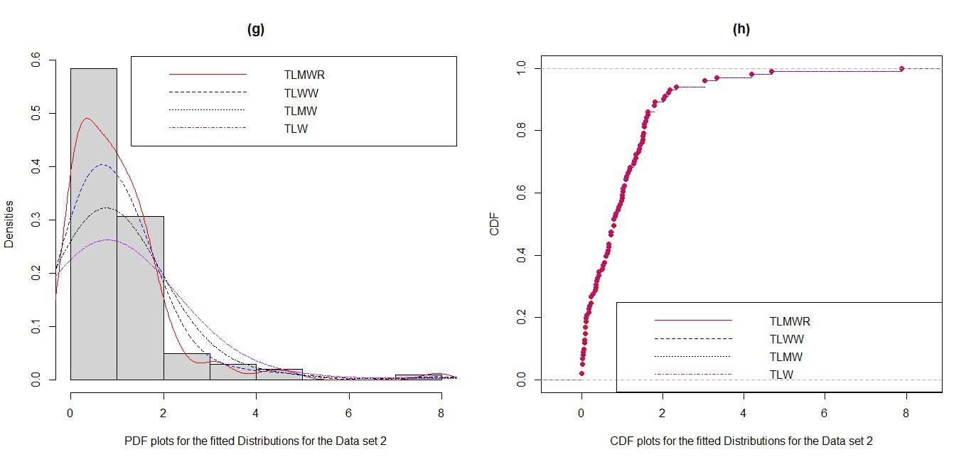
The performance of the model is validated with two real data sets. The first data set consists of survival times (in days) of 72 guinea pigs infected with virulent tubercle bacilli [7]. The second data set consists of 101 observations representing failure times (in hours) of Kevlar 49/epoxy strands subjected to constant sustained pressure at the 90 percent stress level, as reported in [29– 31].
| Distribution | Acronym | References |
|---|---|---|
| Topp-Leone Modified Weighted Rayleigh | TLMWR | Proposed |
| Topp-Leone Modified Weibull | TLMW | [18] |
| Topp-Leone Weibull | LTW | [13] |
| Topp-Leone Weighted Weibull | TLWW | [7] |
| Model | Estimate | W* | A* | KS |
|---|---|---|---|---|
| TLMWR (proposed) | \(\hat{\lambda}=2.2196\,(0.3493^*)\) | |||
| \(\hat{\alpha}=-0.2636\,(4.2868^*)\) | 0.1672 | 0.9810 | 0.2199 | |
| \(\hat{\beta}=-0.7395\,(16.3073^*)\) | \(0.0019^P\) | |||
| \(\hat{\gamma}=-1.7829\,(12.8803^*)\) | ||||
| TLW [13] | \(\hat{\lambda}=65.5971\,(72.9469^*)\) | |||
| \(\hat{\alpha}=0.3475\,(0.1008^*)\) | 0.1667 | 1.1811 | 0.1381 | |
| \(\hat{\beta}=1.9894\,(0.5673^*)\) | \(0.1285^P\) | |||
| \(\hat{\gamma}=1\) | ||||
| TLMW [18] | \(\hat{\lambda}=2.4390\,(0.5818^*)\) | |||
| \(\hat{\alpha}=0.3924\,(0.0771^*)\) | 0.2058 | 1.2187 | 0.0934 | |
| \(\hat{\beta}=3.3623\,(0.4914^*)\) | \(0.5567^P\) | |||
| \(\hat{\gamma}=0.0074\,(0.0006^*)\) | ||||
| TLWW [7] | \(\hat{\lambda}=2.6541\,(1.5369^*)\) | |||
| \(\hat{\alpha}=0.3311\,(4.8472^*)\) | 0.0903 | 0.5609 | 0.0891 | |
| \(\hat{\beta}=1.1603\,(0.3090^*)\) | \(0.6168^P\) | |||
| \(\hat{\gamma}=0.3665\,(19.4499^*)\) |
| Model | \(-2\log L\) | AIC | CAIC | BIC | HQIC | Rank |
|---|---|---|---|---|---|---|
| TLMWR | 35.1597 | 78.3193 | 78.9163 | 87.4260 | 81.9447 | 1st |
| TLW | 82.8643 | 171.7285 | 172.0815 | 178.5585 | 174.4476 | 2nd |
| TLMW | 84.2603 | 176.5206 | 177.1176 | 185.6273 | 180.1460 | 3rd |
| TLWW | 94.0838 | 196.1677 | 196.7647 | 205.2743 | 199.7931 | 4th |
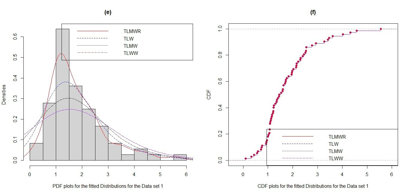
These plots show the density and distribution functions of the models for the first data set in Figure 3. Meanwhile, it is clear from each figure that the TLMWR model fits the data set better than the other models.
| Model | Estimate | W* | A* | KS |
|---|---|---|---|---|
| TLMWR | \(\hat{\lambda}=0.4280\,(0.0479^*)\) | |||
| (proposed) | \(\hat{\alpha}=0.1650\,(2.8531^*)\) | 0.1842 | 1.4223 | 0.1029 |
| \(\hat{\beta}=2.4465\,(\mathrm{NaN}^*)\) | \(0.2354^P\) | |||
| \(\hat{\gamma}=-04614\,(\mathrm{NaN}^*)\) | ||||
| TLW | \(\hat{\lambda}=369.6662\,(149.8551^*)\) | |||
| [13] | \(\hat{\alpha}=0.1748\,(0.0167^*)\) | 0.1482 | 1.0405 | 0.1282 |
| \(\hat{\beta}=2.1981\,(0.1978^*)\) | \(0.0747^P\) | |||
| \(\hat{\gamma}=1\) | ||||
| TLMW | \(\hat{\lambda}=157.7878\,(76.0571^*)\) | |||
| [18] | \(\hat{\alpha}=1.0953\,(0.0884^*)\) | 4.8427 | 24.0037 | 0.8131 |
| \(\hat{\beta}=-0.1723\,(0.0253^*)\) | \(<2.2\mathrm{e}{-16}^P\) | |||
| \(\hat{\gamma}=1.4963\,(0.2229^*)\) | ||||
| TLWW | \(\hat{\lambda}=0.7940\,(0.2872^*)\) | |||
| [7] | \(\hat{\alpha}=0.2521\,(\mathrm{NaN}^*)\) | 0.1654 | 0.9595 | 0.0845 |
| \(\hat{\beta}=1.0594\,(0.2394^*)\) | \(0.4658^P\) | |||
| \(\hat{\gamma}=0.6287\,(\mathrm{NaN}^*)\) |
| Model | -2LogL | AIC | CAIC | BIC | HQIC | Rank |
|---|---|---|---|---|---|---|
| TLMWR | 73.9238 | 155.8476 | 156.2643 | 166.3081 | 160.0823 | 1st |
| TLW | 162.0503 | 330.1006 | 330.3506 | 337.9161 | 333.26376 | 4th |
| TLMW | 86.3654 | 180.7307 | 181.1474 | 191.1912 | 184.9654 | 2nd |
| TLWW | 102.7872 | 213.5744 | 213.9910 | 224.0348 | 217.8091 | 3rd |
In this paper, several model comparison criteria were considered to evaluate the performance of the proposed distribution. These include goodness-of-fit statistics such as the Anderson-Darling (A*), Cramér–von Mises (W*), and Kolmogorov–Smirnov (KS) tests, as well as model selection measures including the log-likelihood \(-2\log l\), Akaike Information Criterion (AIC), Consistent Akaike Information Criterion (CAIC), Bayesian Information Criterion (BIC), and Hannan–Quinn Information Criterion (HQIC), applied to two different data sets.
The adequacy and superiority of a statistical model are generally judged by smaller values of A*, W*, KS, AIC, CAIC, BIC, and HQIC, and by a larger log-likelihood value. Results presented in Tables 7–10 indicate that the proposed TLMWR distribution consistently provides the highest log-likelihood and the lowest values for the goodness-of-fit and model selection statistics. This clearly demonstrates the superior flexibility and fitting ability of the TLMWR distribution compared to the Topp–Leone Weighted Weibull (TLWW), Topp–Leone Modified Weibull (TLMW), and Topp–Leone Weibull (TLW) distributions across both data sets.
Furthermore, the fitted probability density functions (pdfs) and cumulative distribution functions (cdfs) displayed in Figures 3 and 4 visually confirm the empirical results. The TLMWR distribution shows a closer alignment with the observed data than its competing models, thereby reinforcing its practical applicability and statistical relevance. Above-all, these findings establish the robustness and nobility of the proposed model. Its performance in terms of both statistical criteria and graphical assessment highlights its potential as a more reliable alternative for modeling lifetime and reliability data compared to existing Topp–Leone family distributions.
This study introduced and investigated the Topp–Leone Modified Weighted Rayleigh (TLMWR) distribution as a new extension within the Topp–Leone family of distributions. Theoretical properties of the distribution, including its probability density function, cumulative distribution function, survival function, hazard rate, moments, and order statistics, were derived and studied in detail. These mathematical results demonstrate that the TLMWR distribution possesses flexible structural characteristics that allow it to model a wide range of lifetime and reliability data.
To validate its applicability, the TLMWR distribution was fitted to two real data sets and compared with existing related models such as the Topp -Leone Weighted Weibull (TLWW), Topp-Leone Modified Weibull (TLMW), and Topp Leone Weibull (TLW) distributions. The evaluation was based on both goodness-of-fit measures (A*, W*, KS) and model selection criteria (log-likelihood, AIC, CAIC, BIC, HQIC). The empirical results revealed that the TLMWR distribution consistently outperformed the competing models by yielding the largest log-likelihood and the smallest values of the statistical criteria considered. The fitted pdf and cdf plots further confirmed the superior performance of the proposed distribution in capturing the behavior of the observed data.
The superiority of the TLMWR distribution can be attributed to its additional flexibility, which enables it to accommodate various shapes of hazard functions and tail behaviors. This makes the model particularly useful for practical applications in fields such as reliability engineering, survival analysis, medical statistics, and risk assessment, where accurate lifetime modeling is essential. In conclusion, the TLMWR distribution is a noble and powerful alternative within the Topp–Leone family of models. Its strong performance across multiple criteria highlights its robustness and practical relevance. Future research may explore its multivariate extensions, regression structures, Bayesian estimation, and applications to larger and more diverse real-life data sets to further broaden its scope and impact.
Let \[\begin{aligned} f_{TLMWR}(x)= 2\lambda(2\alpha(1+\beta\gamma^{2}))x{e^{-2\alpha(1+\beta\gamma^{2})x^{2}}}\left[1-e^{-2\alpha(1+\beta\gamma^{2})x^{2}}\right]^{\lambda-1}. \end{aligned}\]
Also, setting \(w=2\alpha(1+\beta\gamma^{2}) \therefore w > 0 \quad \text{if} \quad \alpha > 0 \quad \text{and} \quad 1+\beta\gamma^{2} > 0.\)
Then, \[\begin{aligned} f_{TLMWR}(x)= 2\lambda{w}x{e^{-{w}x^{2}}}\left[1-e^{-{w}x^{2}}\right]^{\lambda-1} , \end{aligned}\] We compute the integral over \(x \geq 0.\) \[\begin{aligned} \int_{0}^{\infty}f_{TLMWR}(x)dx=\int_{0}^{\infty}2\lambda{w}x{e^{-{w}x^{2}}}\left[1-e^{-{w}x^{2}}\right]^{\lambda-1}dx . \end{aligned}\]
By using substitution method, we have: \(v=1-e^{-{w}x^{2}}\Rightarrow{dv}=2{w}{x}e^{-{w}x^{2}}dx\) .
If \(x=0, \quad \text{we have} \quad v=0, \quad \text{when} \quad x \to \infty, e^{-{w}x^{2}} \to 0 \quad \text{that is} \quad v \to 1\) .
Therefore, the integrand transforms as \[\begin{aligned} 2\lambda{w}xe^{-{w}x^{2}}dx=\lambda{dv}. \end{aligned}\]
Thus, \[\begin{aligned} \int_{0}^{\infty}f_{TLMWR}(x)dx=\int_{v=0}^{1}\lambda{v^{\lambda-1}}dv=\lambda\left[\dfrac{v^{\lambda}}{\lambda}\right]_{0}^{1}=1. \end{aligned}\]
Finally, \[\begin{aligned} \int_{0}^{\infty}f_{TLMWR}(x)dx=1 \quad \textbf{QED}. \end{aligned}\]
This implies \(f_{TLMWR}(x)\) is a true valid pdf.
Recall, the pdf is \[\begin{aligned} f_{TLMWR}(x)= 2\lambda{w}x{e^{-{w}x^{2}}}\left[1-e^{-{w}x^{2}}\right]^{\lambda-1}, \quad x \geq 0 . \end{aligned}\]
The CDF is \[\begin{aligned} F_{TLMWR}(x)= \int_{0}^{x}f_{TLMWR}(t)dt=\int_{0}^{x}2\lambda{w}t{e^{-{w}t^{2}}}\left[1-e^{-{w}t^{2}}\right]^{\lambda-1}dt . \end{aligned}\]
We use the substitution method \(v=1-e^{-{w}t^2}\). Here, we have \(dv=2w{t}e^{-{w}t^2}dt\), and when \(t=0\) we get \(v=0\), when \(t=x\) also we have \(v=1-e^{-{w}x^2}\). The integrand becomes \(\lambda{v}^{\lambda-1}dv\), Then \[\begin{aligned} F_{TLMWR}(x)= \int_{0}^{1-e^{-{w}x^2}}\lambda{v}^{\lambda-1}dv=\left[v^{\lambda}\right]_{0}^{1-e^{-{w}x^2}}=\left(1-e^{-{w}x^2}\right)^\lambda . \end{aligned}\]
So, the CDF is given by \[\begin{aligned} F_{TLMWR}(x)=\left(1-e^{-{w}x^2}\right)^\lambda, \quad x \geq 0 \end{aligned}\] \[\begin{aligned} \dfrac{d}{dx}F_{TLMWR}(x)=\left(1-e^{-{w}x^2}\right)^\lambda=\lambda\left(1-e^{-{w}x^2}\right)^{\lambda-1}\left(2{w}x{e^{-{w}x^{2}}}\right) . \end{aligned}\]
Differentiating with respect to \(\lambda\) yield, \[\begin{aligned} \dfrac{d}{dx}F_{TLMWR}(x)=\lambda\left(1-e^{-{w}x^2}\right)^{\lambda-1}\left(2{w}x{e^{-{w}x^{2}}}\right)=F_{TLMWR}(x) \quad \textbf{QED} . \end{aligned}\]
They can be written with constraints as follows:
\(\bullet \quad \quad \alpha > 0.\)
\(\bullet \quad \quad \lambda > 0.\)
\(\bullet \quad \quad 1+\beta{\gamma}^{2} > 0.\)
\(\bullet \quad \quad \gamma \in \mathbb{R}.\)
Also, by introducing unconstrained parameters \(\varphi\), we have
\(\bullet \quad \quad \alpha =e^{\varphi_{\alpha}} \quad \text{certainly} \quad \alpha > 0\) .
\(\bullet \quad \quad \lambda =e^{\varphi_{\lambda}} \quad \text{certainly} \quad \lambda > 0\) .
\(\bullet \quad \quad \beta =e^{\varphi_{\beta}} \quad \text{certainly} \quad \beta > 0, \quad \text{hence} \quad 1+\beta{\gamma^2} > 1 > 0\) .
\(\bullet \quad \quad \gamma ={\varphi_{\gamma}} \in \mathbb{R}\) .
For example, reparameterized the negative log-likelihood with simulated data of 100 data points using the exponent \(W=2\alpha(1+\beta\gamma^2)\). Then the MLEs of the parameters are:
\(\bullet \quad \quad \hat{\alpha} = 0.3671996\) . \(\bullet \quad \quad \hat{\beta} = 1.0\) .
\(\bullet \quad \quad \hat{\gamma} = -1.9589×10^{-8} \approx 0\) .
\(\bullet \quad \quad \hat{\lambda} = 1.1366108\).
Checking the parameter domains using earlier valid domain conditions as follows:
\(\bullet \quad \quad \alpha > 0 \quad \text{\textbf{satisfied}} \quad (0.367 > 0)\).
\(\bullet \quad \quad \lambda > 0 \quad \text{\textbf{satisfied}} \quad (1.137 > 0)\).
\(\bullet \quad \quad 1+\beta{\gamma}^{2} > 0 \quad \text{with} \quad \beta=1 \quad \text{and} \quad \gamma=0, \text{this is} \quad 1+1.0 \approx 1 > 0 -\text{\textbf{satisfied}}\).
\(\bullet \quad \quad \gamma \in \mathbb{R} \quad – good\).
The estimates are inside the nominal feasible region. These values imply that the likelihood expression \(W \equiv 2\alpha(1+\beta\gamma^2)\) and the estimates is:
\(\bullet \quad \quad 1+\beta{\gamma}^{2} \approx 1 + 1 \times (0)^2 = 1\).
\(\bullet \quad \quad \text{Now}, W=2\alpha = 2\times 0.3671996=0.7343992\).
Then, the penalty term in the log-likelihood \(-W\sum\limits_{i}{x_{i}^{2}}\) is being multiplied by approximately 0.7344. The data dependent penalization on \(\sum{x_{i}^{2}}\) is sealed by \(\simeq 0.7344\). Python code generate the estimates are in the appendix.
Suppose the log-likelihood function of TLMWR distribution \(LL_{TLMWR}(\theta)= LL_{TLMWR}{(\alpha, \beta, \gamma, \lambda)}\) with parameter vector \(\theta \in \mathbb{R}^{p}\).
The observed information matrix is the negative of the Hessian of the log-likelihood at the MLE: \[\begin{aligned} I_{obs}{(\hat{\theta})}= {-\dfrac{\partial^{2}LL_{TLMWR}(\theta)}{\partial{\theta}\partial{\theta}^{T}}}\bigg|_{\theta={\hat{\theta}}}. \end{aligned}\]
Appriximate covariance matrix of the MLE: \[\begin{aligned} \hat{Var}{\hat{(\theta)}}=I_{obs}\hat{{(\theta)}^{-1}} . \end{aligned}\]
For each parameter \(\theta_{j}:\) \[\begin{aligned} SE{\hat{(\theta_{j})}}= \sqrt{\left(\hat{Var}\hat{(\theta)}\right)_{jj}}. \end{aligned}\]