Abstract
1. Introduction
2. Problem formulation and mathematical analysis
3. Method of solution: Two-dimensional differential transformation method
4. Results and discussion
5. Conclusion
Abbreviations: Nomenclature
References

Engineering and Applied Science Letters (EASL)

Volume 3 (2020) Issue 1
Pages: 1
- 20

ISSN: 2617-9709 (Online) 2617-9695 (Print)

DOI: https://www.doi.org/10.30538/psrp-easl2020.0031

Research article

Dynamic analysis of non-homogenous varying thickness rectangular plates resting on Pasternak and Winkler foundations

Author(s): ^¹, ^², ^¹

¹Department of Civil and Environmental Engineering, University of Lagos, Akoka, Nigeria.

²Department of Mechanical Engineering, University of Lagos, Akoka, Nigeria.

Copyright © S. A. Salawu, M. G. Sobamowo, O. M. Sadiq. This is an open access article distributed under the Creative Commons Attribution License, which permits unrestricted use, distribution, and reproduction in any medium, provided the original work is properly cited.

Received: 26/05/2019
Accepted: 30/12/2019
Published: 22/02/2020

Abstract

Modern day technological advancement has resulted in manufacturing industries intensify the use and application of thin plates in their productions thereby, resulting in increased research awareness in the study of dynamic behavior of thin plates. This research analyzes the free vibration dynamic behavior of thin rectangular plates resting on elastic Winkler and Pasternak foundations using two-dimensional differential transformation method. The reliability of the obtained analytical solutions are validated with results presented in cited literature and confirmed very precise. However, the analytical solutions obtained are used to investigate the influence of elastic foundations, homogeneity and thickness variation on the dynamic behavior of the plates under clamped and condition. From the results obtained, it is realized that increase in non-homogenous material results in corresponding increase in natural frequency of the plates. Also, increase in Winkler, Pasternak and combine Winkler and Pasternak foundations stiffness leads to increase in natural frequency of the plates. Increase in thickness results to natural frequency increases. The findings will serve as benchmark for further study of plate vibration research.

Keywords: Natural frequencies, nonlinear free vibration, thin plate, Winkler and Pasternak foundations, two-dimensional differential transformation method.

1. Introduction

Reduction in size, weight and varying density of plates had proven to be of good economic advantage in engineering design. These factors result into better strength, bending, vibration, buckling and guide against resonance as compared to uniform thickness homogenous plates. Also, these increases the utilization of non-homogenous varying thickness plates in engineering fields and industries [1]. In the interest of determining the dynamic analysis of non-homogenous varying thickness rectangular plates, [2-6] investigated the study using analytical method of solution.

The study of structures resting on foundations is of great importance to geotechnics and foundation engineers. However, in the model of foundation in engineering, adoption of Winkler foundation is mostly common which suffers challenge of continuous soil pressure [7]. Reason being that, shear deformation normally occurs in Winkler foundation. To put this wrong assumption in order, designers now introduced Pasternak foundation to support the linear elastic Winkler foundation. However, Sakiyama and Huang [8] utilized green function, a numerical approach to investigate analysis of rectangular plate resting on Winkler foundation. In a further research, Amini et al. [9] showed the power of Chebyshev polynomial and Ritz method in evaluating the analysis of functional graded material rectangular plates on elastic foundation. Bahmyari and Rahbar-Ranji [10] applied Galerkin free element method into the vibration analysis of Orthotropic plates of non-uniform thickness resting on Winkler foundation. In another work, Sharma et al. [11] used differential quadrature solution approach to investigate the behavior of rectangular plate on a Winkler foundation.

Research into dynamic behavior of plates dated back as far as 1800, when Euler first postulated mathematical model for membrane. Thereafter, Lagrange formulated plates governing equation [12]. Furthermore, numerous works had been published in the field. Meanwhile, at initial phase of the research, interest was on simple cases where exact solution can be provided. Chakravery [1] pointed-out that, due to lack of fast computing tools, results obtained for simple cases were not precise, complex cases of vibration problems were left out. This may have led to gap in numerical solution for complex cases of vibration problem despite technological advancement and availability of fast computing tools. It is therefore justified to apply various newly discovered method of solutions in obtaining results for complex and simple cases of vibration problem. Based on literatures reviewed, nonlinear governing differential equations cannot be analyzed using analytical method due to complex mathematics involved. Numerical method has an edge tackling the problem, but it is time consuming with huge cost implication. Nevertheless, in the quest to provide symbolic solutions, Ogunjiofor and Nwoji [13] used characteristic polynomial, a semi-analytical method of solutions to analyze the vibration of plates resting on Winkler foundations. In another study, Matsuda and Sakiyama [14] investigated bending analysis of non-uniform thickness rectangular plates resting on elastic foundation. Furthermore, Miandoab et al. [15] used Homotopy analysis method (HAM) in conducting forced vibration analysis on nanoplates. Thereafter, Rahbar and Rostami [16] discussed vibration response of rectangular orthotropic plates using HAM. HAM suffers limitation of auxiliary parameters and initial approximation. Differential transformation method (DTM), a semi analytical method proposed by Zhou [17] for initial ordinary differential equation, which was later extended to partial differential equation [18], is a reliable method of solution, simple to use without discretization, restrictive assumptions, linearization, perturbation and round-off-error. It reduces complex governing equations into an algebraic equation. Therefore, [19,20] applied DTM on initial value problems of partial differential equations.

The research focuses on application of two-dimensional DTM to nonlinear dynamic behavior of non-homogeneous, non-uniform thickness plate resting on elastic Winkler and Pasternak foundations to establish approximate analytical solutions and parametric studies carried out on the controlling parameters.

2. Problem formulation and mathematical analysis

Considering isotropic rectangular plate of varying thickness shown in Figure 1 resting on two-parameter foundations. Clamped edge boundary condition is considered in this study. The length and width are represented as $a$ and $b$ respectively. The governing differential equation of a thin varying thickness rectangular plate as given by [21] is;

$\begin{matrix} (1) & \begin{aligned} \frac{\partial^{2}}{\partial x^{2}} [- D (\frac{\partial^{2} w}{\partial x^{2}} + ν \frac{\partial^{2} w}{\partial y^{2}})] + 2 \frac{\partial^{2}}{\partial x \partial y} [- D (1 - ν) (\frac{\partial^{2} w}{\partial x \partial y})] + \frac{\partial^{2}}{\partial y^{2}} [- D (\frac{\partial^{2} w}{\partial y^{2}} + ν \frac{\partial^{2} w}{\partial x^{2}})] + k_{w} w \\ - k_{s} (\frac{\partial^{2} w}{\partial x^{2}} + \frac{\partial^{2} w}{\partial y^{2}}) + k_{p} w^{3} = - ρ h ω^{2} + \frac{ρ h^{3} ω^{2}}{12} (\frac{\partial^{2} w}{\partial x^{2}} + \frac{\partial^{2} w}{\partial y^{2}}) \end{aligned} \end{matrix}$ where $D = \frac{E h^{3}}{12 (1 - ν^{2})}$ is the flexural rigidity, $E$ represents the modulus of rigidity, $ρ$ represents the density, $h$ is the thickness, $w (x, y)$ represents the transverse deflection and $ω$ represents the natural frequency, Poisson’s ratio $v$ , shear Pasternak $k_{s}$ , Winkler stiffness $k_{w}$ and $k_{p}$ represents nonlinear Winkler stiffness coefficient.

Assuming the thickness and density varies linearly in the direction as:

$\begin{matrix} (2) & \begin{aligned} h (x, y) = p_{o} (1 + β \frac{x}{a}) and homogeneity parameter is ρ = ρ_{o} (1 + α_{1} \frac{x}{a}) \end{aligned} \end{matrix}$ where $α_{1}$ is the non-homogeneity parameter and, $β$ is the taper parameter. Therefore, flexural rigidity may be written as [22]:

where the flexural rigidity $D = \frac{E h^{3}}{12 (1 - ν^{2})}$ . Assuming $μ = \frac{E h_{m}^{3}}{12 (1 - v^{2})}$ then, $D = μ [h (x, y)]^{3}$ . Therefore,

$\begin{matrix} (3) & \begin{aligned} D = μ [1 + \frac{3 x β}{a} + \frac{3 x^{2} β^{2}}{a^{2}} + \frac{x^{3} β^{3}}{a^{3}}] \end{aligned} \end{matrix}$

Applying Equation (2) and (3) on Equation (1), we have:

$\begin{matrix} (4) & \begin{aligned} \frac{\partial^{2}}{\partial x^{2}} [- μ h^{3} (\frac{\partial^{2} w}{\partial x^{2}} + ν \frac{\partial^{2} w}{\partial y^{2}})] + 2 \frac{\partial^{2}}{\partial x \partial y} [- μ h^{3} (1 - ν) (\frac{\partial^{2} w}{\partial x \partial y})] + \frac{\partial^{2}}{\partial y^{2}} [- μ h^{3} (\frac{\partial^{2} w}{\partial y^{2}} + ν \frac{\partial^{2} w}{\partial x^{2}})] + k_{w} w \\ - k_{s} (\frac{\partial^{2} w}{\partial x^{2}} + \frac{\partial^{2} w}{\partial y^{2}}) + k_{p} w^{3} = - ρ h w ω^{2} + \frac{ρ h^{3} ω^{2}}{12} (\frac{\partial^{2} w}{\partial x^{2}} + \frac{\partial^{2} w}{\partial y^{2}}) \end{aligned} \end{matrix}$

Applying product rule on the Equation (4), we obtained: $\begin{matrix} (5) & \begin{aligned} μ h^{3} (\frac{\partial^{4} w}{\partial x^{4}} + 2 ν \frac{\partial^{4} w}{\partial x^{2} \partial y^{2}} + \frac{\partial^{4} w}{\partial y^{2}}) + 2 μ \frac{\partial h^{3}}{\partial x} (\frac{\partial^{3} w}{\partial x^{3}} + ν \frac{\partial^{3} w}{\partial y^{2} \partial x}) + 2 μ \frac{\partial h^{3}}{\partial y} (\frac{\partial^{3} w}{\partial y^{3}} + ν \frac{\partial^{3} w}{\partial x^{2} \partial y}) + μ \frac{\partial^{2} h^{3}}{\partial x^{2}} (\frac{\partial^{2} w}{\partial x^{2}} \\ + ν \frac{\partial^{2} w}{\partial y^{2}}) + μ \frac{\partial^{2} h^{3}}{\partial y^{2}} (\frac{\partial^{2} w}{\partial y^{2}} + ν \frac{\partial^{2} w}{\partial x^{2}}) + 2 μ h^{3} (1 - ν) \frac{\partial^{4} w}{\partial x^{2} \partial y^{2}} + 2 μ (1 - ν) \frac{\partial h^{3}}{\partial x} \frac{\partial^{3} w}{\partial x \partial y^{2}} + 2 μ (1 - ν) \frac{\partial h^{3}}{\partial y} \frac{\partial^{3} w}{\partial x^{2} \partial y} \\ + 2 μ (1 - ν) \frac{\partial^{2} h^{3}}{\partial x \partial y} \frac{\partial^{2} w}{\partial x \partial y} + k_{w} w - k_{s} (\frac{\partial^{2} w}{\partial x^{2}} + \frac{\partial^{2} w}{\partial y^{2}}) + k_{p} w^{3} = ρ h w ω^{2} - \frac{ρ h^{3} ω^{2}}{12} (\frac{\partial^{2} w}{\partial x^{2}} + \frac{\partial^{2} w}{\partial y^{2}}) . \end{aligned} \end{matrix}$

Applying the non-dimensionless parameters, $ξ = \frac{x}{a}$ , $η = \frac{y}{b}$ , $k_{w} = \frac{a^{4} \bar{k_{w}}}{μ}$ , $k_{s} = \frac{G a^{2}}{μ}$ , $k_{p} = \frac{a^{4} \bar{k_{p}}}{μ}$ and $W = \frac{w}{W_{m a x}}$ on Equation (5), we arrived at:

$\begin{matrix} (6) & \begin{aligned} μ [h_{o} (1 + β \frac{ξ}{a})]^{3} [b^{4} \frac{\partial^{4} W}{\partial ξ^{4}} + 2 a^{2} b^{2} \frac{\partial^{4} W}{\partial ξ^{2} \partial η^{2}} + a^{4} \frac{\partial^{4} W}{\partial η^{4}}] + 2 μ \frac{\partial (h_{o} (1 + β \frac{ξ}{a}))^{3}}{\partial ξ} [b^{4} \frac{\partial^{3} W}{\partial ξ^{3}} + a^{2} b^{4} \frac{\partial^{3} W}{\partial ξ \partial η^{2}}] \\ + μ \frac{\partial ((h_{o} (1 + β \frac{ξ}{a}))^{3})^{2}}{\partial ξ^{2}} [b^{4} \frac{\partial^{2} W}{\partial ξ^{2}} + a^{2} b^{4} ν \frac{\partial^{2} W}{\partial ξ^{2}}] - a^{4} b^{4} ρ_{o} h_{o} (1 + α_{1} \frac{ξ}{a}) (1 + β \frac{ξ}{a}) ω^{2} [W] + a^{4} b^{4} k_{w} W \\ - k_{s} (a^{2} b^{4} \frac{\partial^{2} W}{\partial ξ^{2}} + a^{4} b^{2} \frac{\partial^{2} W}{\partial η^{2}}) + a^{4} b^{4} k_{p} W^{3} + \frac{ρ_{o} h_{o} (1 + α_{1} \frac{ξ}{a}) (1 + β \frac{ξ}{a}) ω^{2}}{12} [a^{2} b^{4} \frac{\partial^{2} W}{\partial ξ^{2}} + a^{4} b^{2} \frac{\partial^{2} W}{\partial η^{2}}] = 0. \end{aligned} \end{matrix}$

2.1 Boundary conditions

Clamped edge condition is considered in this study which. This is presented as follow [23]:
Clamped edge (C): $\begin{matrix} (7) & \begin{aligned} w (x, y) = 0, \frac{\partial w (x, y)}{\partial x} = 0 a t x = 0 o r x = a \end{aligned} \end{matrix}$ $\begin{matrix} (8) & \begin{aligned} w (x, y) = 0, \frac{\partial w (x, y)}{\partial y} = 0 a t y = 0 o r y = a \end{aligned} \end{matrix}$

Table 1 Material properties
Plate
Young’s Modulus GPa	Poisson’s ratio	mass density	Initial thickness	length	width
	$v$	$ρ_{m} \frac{k g}{m^{3}}$	$P_{o} (m m)$	$a (m m)$	$b (m m)$
69.0E9	0.3	2700	0.05	300	200

3. Method of solution: Two-dimensional differential transformation method

Two-dimensional differential transformation method is an improved version of DTM introduced by Zhou [17]. The method can be applied to partial differential equation with ease. The approach is an iterative method. The basic definitions and operational principles are stated as follows: $\begin{matrix} (9) & \begin{aligned} W (k, h) = \frac{1}{k! h!} [\frac{\partial^{k + h} w (x, y)}{\partial x^{k} \partial y^{h}}]_{0, 0}, T - function \end{aligned} \end{matrix}$ where $w (x, y)$ is the original function and $W (k, h)$ is the transformed function.

The differential inverse transform of $W (k, h)$ is defined as: $\begin{matrix} (10) & \begin{aligned} w (x, y) = \sum_{k = 0}^{\infty} \sum_{h = 0}^{\infty} W (x, y) x^{k} y^{h} . \end{aligned} \end{matrix}$

From Equation (9) and (10) leads to: $\begin{matrix} (11) & \begin{aligned} w (x, y) = \sum_{k = 0}^{\infty} \sum_{h = 0}^{\infty} \frac{1}{k! h!} [\frac{\partial^{k + h} w (x, y)}{\partial x^{k} \partial y^{h}}]_{0, 0} x^{k} y^{h} \end{aligned} \end{matrix}$

Table 2 Operational properties of two dimensional differential transformation method
Original function	Transform function
$w (x, y) \pm u (x, y)$	$W (k, h) \pm U (k, h)$
$\frac{\partial w (x, y)}{\partial x}$	$(k + 1) W (k + 1, h)$
$\frac{\partial w (x, y)}{\partial y}$	$(h + 1) W (k, h + 1)$
$\frac{\partial^{r + s} W (x, y)}{\partial x^{r} \partial y^{s}}$	$(k + 1) (k + 2) \dots (k + r) (h + 1) (h + 2) \dots (h + s) W (k + r, h + s)$
$w (x, y) v (x, y)$	$\sum_{r} = 0^{k} \sum_{s} = 0^{h} W (r, h - s) V (k - r, s)$

3.1 Application of DTM to the boundary conditions

Applying the operation properties of two-dimensional DTM mentioned in Table 2 to the condition Equation (7) at $x = 0$ . As expected, for $n$ -th order differential governing equation, $n$ -th number of conditions are required for the analysis. Therefore, for Equation (6), two remaining unknown conditions are represented with constant variables which are found later.
Clamped Support condition: $\begin{matrix} (12) & \begin{aligned} W (k, h) = 0 \Rightarrow W (0, h) = 0, \end{aligned} \end{matrix}$ $\begin{matrix} (13) & \begin{aligned} (k + 1) W (k + 1, h) = 0 \Rightarrow W (1, h) = 0. \end{aligned} \end{matrix}$

Therefore, to obtain the four conditions required to analyze fourth-order differential equation as stated earlier, two unknowns are introduced more, we have: $\begin{matrix} (14) & \begin{aligned} (k + 1) (K + 2) W (K + 2, h) = a_{1} \Rightarrow W (2, h) = a_{1}, \end{aligned} \end{matrix}$ $\begin{matrix} (15) & \begin{aligned} (k + 1) (k + 2) (k + 3) W (k + 3, h) = b_{1}, \Rightarrow W (3, h) = b_{1} . \end{aligned} \end{matrix}$

Therefore, the transformed boundary conditions are: $\begin{matrix} (16) & \begin{aligned} W (0, h) = 0; W (1, h) = 0; W (2, h) = a_{1}; W (3, h) = \frac{b_{1}}{6} . \end{aligned} \end{matrix}$

3.2. Application of two-dimensional differential transformation method to the governing equation under investigation

Applying the operational properties in Table 1, the two-dimensional DTM transform of the governing equation Equation (6) is resolved as:
$W_{k + 4, h} = \frac{1}{μ b^{4} {p_{0}}^{3} (k + 1) (k + 2) (k + 3) (k + 4) W (k + 4, h)} \times [(\frac{3 μ b^{4} β {p_{0}}^{3} (k + 1) {(k + 2)}^{2} (k + 3)}{a}) W (k + 3, h) + 2 a^{2} b^{2} μ {p_{0}}^{3} (k + 1) (k + 2) (h + 1) (h + 2) W (k + 2, h + 2) + 12 μ a b^{2} β {p_{0}}^{3} (k + 1) k W (k + 1, 2) + (\frac{4 μ b^{2} β^{3} {p_{0}}^{3} (k - 1) (3 b^{2} + k - 2)}{a}) W (k - 1, 2) + μ a^{4} {p_{0}}^{3} (h + 1) (h + 2) (h + 3) (h + 4) W (k, h + 4) + 3 β μ a^{3} {p_{0}}^{3} (h + 1) (h + 2) (h + 3) (h + 4) W (k - 1, h + 4) + 3 β^{2} μ a^{2} {p_{0}}^{3} (h + 1) (h + 2) (h + 3) (h + 4) W (k - 2, h + 4) + β^{3} μ a {p_{0}}^{3} (h + 1) (h + 2) (h + 3) (h + 4) W (k - 3, h + 4) + 6 μ a b^{4} β {p_{0}}^{3} (k + 1) (h + 1) (h + 2) W (k + 1, h + 2) + (12 μ b^{2} β^{2} {p_{0}}^{3} k (2 b^{2} + k - 1)) W (k, 2) + (- \frac{(k + 1) (k + 2) ((- \frac{1}{12} a^{4} ω^{2} ρ_{0} - 3 β^{2} k^{2} μ - 9 β^{2} k μ - 6 β^{2} μ) {p_{0}}^{3} + k_{s} a^{4}) b^{4}}{a^{2}}) W (k + 2, h) + (- (h + 1) (h + 2) b^{2} ((- \frac{1}{12} a^{4} ω^{2} ρ_{0} - 6 β^{2} μ ν) {p_{0}}^{3} + k_{s} a^{4})) W (k, h + 2) + a^{4} b^{4} k_{p} (\sum_{l = 0}^{k} \sum_{p = 0}^{k - l} \sum_{r = 0}^{h} \sum_{s = 0}^{h - r} W (l, h - r - s) W (p, r) W (k - l - p, s)) - (\frac{ω^{2} α_{1} (a^{4} p_{0} + \frac{1}{12} {p_{0}}^{3} β^{2} (k - 3) (k - 2)) ρ_{0} b^{4}}{a^{2}}) W (k - 2, h) + (\frac{1}{4} \frac{{p_{0}}^{3} (k + 1) k (4 μ (k + 2) (k + 1) β^{3} + a^{4} β ω^{2} ρ_{0} + \frac{1}{3} ρ_{0} ω^{2} a^{4} α_{1}) b^{4}}{a^{3}}) W (k + 1, h) + b^{4} (- (- \frac{1}{2} k β {p_{0}}^{3} (k - 1) α_{1} + a^{4} p_{0}) ω^{2} ρ_{0} + a^{4} k_{w}) W (k, h) - \frac{ω^{2} (- \frac{1}{12} {p_{0}}^{3} (k - 1) (k - 2) β^{3} - \frac{1}{4} {p_{0}}^{3} α_{1} (k - 1) (k - 2) β^{2} + p_{0} β a^{4} + p_{0} a^{4} α_{1}) ρ_{0} b^{4}}{a} W (k - 1, h) + (\frac{1}{12} \frac{((h + 1) {p_{0}}^{3} (h + 2) ω^{2} ρ_{0} α_{1} + 3 β a^{4} + 72 β^{3} μ ν) b^{2}}{a}) W (k - 1, h + 2) + \frac{1}{4} ρ_{0} {p_{0}}^{3} ω^{2} a^{2} b^{2} β (h + 2) (h + 1) (β + α_{1}) W (k - 2, h + 2) + \frac{1}{12} ρ_{0} {p_{0}}^{3} ω^{2} a b^{2} β^{2} (h + 2) (h + 1) (β + 3 α_{1}) W (k - 3, h + 2) + \frac{1}{12} ρ_{0} {p_{0}}^{3} ω^{2} b^{2} β^{3} α_{1} (h + 1) (h + 2) W (k - 4, h + 2)] .$ $\begin{aligned} \end{aligned}$

3.3. The solution

Applying fixed value of $h$ and varying $k$ from 0 to 8 on Equation (17). Similarly reverse the process by varying values of $h$ from 0 to 8 while $k$ is fixed, the following equations are developed: $\begin{matrix} (18-28) & \begin{aligned} W_{4, 0} & = & - 5 β a_{1} - \frac{1}{40} β b_{1}, \\ W_{5, 0} & = & \frac{6997 β^{2} a_{1}}{10000} + \frac{3 β^{2} b_{1}}{1000} - \frac{b_{1}}{30} - \frac{a_{1}}{5} - \frac{b_{1} ω^{2}}{32967033} + \frac{4 b_{1} k_{s}}{10989011} + \frac{4262 a_{1} ω^{2}}{292721} + \frac{8 a_{1} k_{s}}{10989011} - \frac{91 a_{1} k_{w}}{2500000}, \\ W_{6, 0} & = & - \frac{β^{3} b_{1}}{3000} - \frac{2}{15} W_{4, 2} - \frac{4997 β^{3} a_{1}}{60000} - \frac{849 β a_{1} ω^{2}}{349951} - \frac{103 β a_{1} k_{s}}{13870933} + \frac{80 β a_{1} k_{w}}{10989011} - \frac{b_{1} ω^{2} α_{1}}{989010989} \\ + \frac{270 a_{1} ω^{2} α_{1}}{556321} + \frac{β b_{1} ω^{2}}{164835165} - \frac{6 β b_{1} k_{s}}{54945055} - \frac{49 β b_{1}}{300} + \frac{19999999 β a_{1}}{999999951}, \\ W_{7, 0} & = & - \frac{431 β a_{1} ω^{2} α_{1}}{4145274} + \frac{β b_{1} ω^{2} α_{1}}{11538461539} + \frac{9 ω^{2} a_{1} k_{s}}{594362519} + \frac{ω^{2} a_{1} k_{w}}{316990701874} + \frac{4 β^{2} b_{1} k_{s}}{187617261} \\ - \frac{k_{s} a_{1} k_{w}}{26415891821} - \frac{β^{2} b_{1} ω^{2}}{1357466065} - \frac{ω^{2} b_{1} k_{s}}{15849535093702} - \frac{13 b_{1} k_{w}}{15000000} + \frac{a_{1} {k_{s}}^{2}}{1320794591072} \\ + \frac{b_{1} {k_{s}}^{2}}{2641589182144} - \frac{ω^{4} a_{1}}{792480056} + \frac{ω^{4} b_{1}}{380388842345313} - \frac{13 k_{p} {a_{1}}^{3}}{2500000} - \frac{14 β W_{4, 2}}{25} + \frac{4685 β^{4} a_{1}}{504888} \\ + \frac{28801 β^{4} b_{1}}{806428001} - \frac{2}{21} W_{5, 2} + \frac{35 β^{2} a_{1} k_{s}}{15161439} - \frac{13 β^{2} a_{1} k_{w}}{12500000} + \frac{577 β^{2} a_{1} ω^{2}}{1850031} + \frac{13 a_{1} ω^{2} α_{1}}{625000} - \frac{b_{1}}{210} \\ + \frac{4 a_{1} ω^{2}}{230769231} + \frac{416 b_{1} ω^{2}}{1199995} - \frac{4 b_{1} k_{s}}{230769231} - \frac{13 a_{1} k_{s}}{62500000} - \frac{554111 β^{2} a_{1}}{242423563} + \frac{2478 β^{2} b_{1}}{117773}, \\ W_{4, 1} & = & - 15 β a_{1} - \frac{1}{40} β b_{1}, \\ W_{4, 2} & = & - 30 β a_{1} - \frac{1}{40} β b_{1}, \\ W_{5, 2} & = & \frac{25991 β^{2} a_{1}}{5000} + \frac{3 β^{2} b_{1}}{1000} - \frac{b_{1}}{5} - 3 a_{1} - \frac{b_{1} ω^{2}}{32967033} + \frac{4 b_{1} k_{s}}{10989011} + \frac{224 a_{1} ω^{2}}{15385} + \frac{48 a_{1} k_{s}}{10989011} - \frac{91 a_{1} k_{w}}{2500000}, \\ W_{4, 3} & = & - 50 β a_{1} - \frac{1}{40} β b_{1}, \\ W_{5, 3} & = & \frac{8797 β^{2} a_{1}}{1000} + \frac{3 β^{2} b_{1}}{1000} - \frac{b_{1}}{3} - 7 a_{1} - \frac{b_{1} ω^{2}}{32967033} + \frac{4 b_{1} k_{s}}{10989011} + \frac{7023 a_{1} ω^{2}}{482369} + \frac{80 a_{1} k_{s}}{10989011} - \frac{91 a_{1} k_{w}}{2500000}, \\ W_{4, 4} & = & - 75 β a_{1} - \frac{1}{40} β b_{1}, \\ W_{5, 4} & = & \frac{26591 β^{2} a_{1}}{2000} + \frac{3 β^{2} b_{1}}{1000} - \frac{b_{1}}{2} - 14 a_{1} - \frac{b_{1} ω^{2}}{32967033} + \frac{4 b_{1} k_{s}}{10989011} + \frac{1390 a_{1} ω^{2}}{95473} + \frac{131 a_{1} k_{s}}{11996337} - \frac{91 a_{1} k_{w}}{2500000} . \end{aligned} \end{matrix}$

Applying DTM principle, we have the solutions of Equation (6) as: $\begin{matrix} (29) & \begin{aligned} W (x, y) = \sum_{j = 0}^{7} \sum_{l = 0}^{6} w (j, l) x^{j} y^{l} . \end{aligned} \end{matrix}$

To validate the analytical solutions obtained using two-dimensional differential transformation method. The controlling parameters in the model are assigned value of zeros. Therefore, substitute $α_{1} = 0, k_{w} = 0, k_{p} = 0, k_{s} =0, β = 0$ into Equation (29), we obtained:
$w (x, y) = \frac{b_{1} x^{3} y^{6}}{6} + \frac{b_{1} x^{3} y^{3}}{6} + \frac{b_{1} x^{3} y}{6} + a_{1} x y^{3} + a_{1} x y + \frac{b_{1} x^{3} y^{4}}{6} + a_{1} x y^{5} + a_{1} x y^{2} + \frac{b_{1} x^{3} y^{2}}{6} + \frac{b_{1} x^{3} y^{5}}{6} + a_{1} x + \frac{b_{1} x^{3}}{6} a_{1} x y^{6} + a_{1} x y^{4} + (- \frac{b_{1}}{30} - \frac{a_{1}}{5} - \frac{b_{1} ω^{2}}{32967033} + \frac{4262 a_{1} ω^{2}}{292721}) x^{5} + (- \frac{b_{1}}{10} - a_{1} - \frac{b_{1} ω^{2}}{32967033} + \frac{5824 a_{1} ω^{2}}{400005}) x^{5} y + (\frac{- b_{1}}{5} - 3 a_{1} - \frac{b_{1} ω^{2}}{32967033} + \frac{224 a_{1} ω^{2}}{15385}) x^{5} y^{2} + (\frac{- b_{1}}{3} - 7 a_{1} - \frac{b_{1} ω^{2}}{32967033} + \frac{7023 a_{1} ω^{2}}{482369}) x^{5} y^{3} + (\frac{- b_{1}}{2} - 14 a_{1} - \frac{b_{1} ω^{2}}{32967033} + \frac{1390 a_{1} ω^{2}}{95473}) x^{5} y^{4} + (- \frac{7 b_{1}}{10} - \frac{126 a_{1}}{5} - \frac{b_{1} ω^{2}}{32967033} + \frac{2920 a_{1} ω^{2}}{200567}) x^{5} y^{5} + (- \frac{14 b_{1}}{15} - 42 a_{1} - \frac{b_{1} ω^{2}}{32967033} + \frac{1603 a_{1} ω^{2}}{110109}) x^{5} y^{6} + (- \frac{1078 a_{1} ω^{2}}{777433} + \frac{416 b_{1} ω^{2}}{1199985} + \frac{ω^{4} b_{1}}{380388842345313} - \frac{ω^{4} a_{1}}{792480056} + \frac{b_{1}}{70} + \frac{2 a_{1}}{7}) x^{7} (- \frac{1669 a_{1} ω^{2}}{401227} + \frac{485 b_{1} ω^{2}}{1398986} + \frac{ω^{4} b_{1}}{380388842345313} - \frac{ω^{4} a_{1}}{792486660} + \frac{b_{1}}{14} + 2 a_{1}) x^{7} y + (- \frac{2628 a_{1} ω^{2}}{315895} + \frac{847 b_{1} ω^{2}}{2443086} + \frac{ω^{4} b_{1}}{380388842345313} - \frac{ω^{4} a_{1}}{792496567} + \frac{3 b_{1}}{14} + 8 a_{1}) x^{7} y^{2} + (- \frac{3356 a_{1} ω^{2}}{242051} + \frac{412 b_{1} ω^{2}}{1188313} + \frac{ω^{4} b_{1}}{380388842345313} - \frac{ω^{4} a_{1}}{792509776} + \frac{b_{1}}{2} + 24 a_{1}) x^{7} y^{3} + (- \frac{3949 a_{1} ω^{2}}{189889} + \frac{3042 b_{1} ω^{2}}{8773355} + \frac{ω^{4} b_{1}}{380388842345313} - \frac{ω^{4} a_{1}}{792526287} + \frac{769230768 b_{1}}{769230769} + 60 a_{1}) x^{7} y^{4} + (- \frac{10141 a_{1} ω^{2}}{348327} + \frac{1045 b_{1} ω^{2}}{3013632} + \frac{ω^{4} b_{1}}{380388842345313} - \frac{ω^{4} a_{1}}{792546102} + \frac{179999998 b_{1}}{99999999} + 132 a_{1}) x^{7} y^{5} + (- \frac{7751 a_{1} ω^{2}}{199687} + \frac{457 b_{1} ω^{2}}{1317808} + \frac{ω^{4} b_{1}}{380388842345313} - \frac{ω^{4} a_{1}}{792569221} + 3 b_{1} + 264 a_{1}) x^{7} y^{6} .$ $\begin{matrix} (30) & \begin{aligned} \end{aligned} \end{matrix}$

Applying the boundary conditions Equation (8) on the series solution. Simultaneous equations are obtained for different step values of $y$ which may be written in this form: for $x = 1$ and $y = \frac{2959}{5000}$ , Equation (30) becomes: $\begin{matrix} (31) & \begin{aligned} W [x, y] = \frac{ω^{4} a_{1}}{22760747346362} + \frac{947 b_{1} ω^{2}}{572106} + \frac{1621 a_{1} ω^{2}}{279789} + \frac{ω^{4} b_{1}}{79662615694136} + \frac{66131 b_{1}}{52363} + \frac{184670 a_{1}}{51349} = 0, \end{aligned} \end{matrix}$ $\begin{matrix} (32) & \begin{aligned} \frac{d W [x, y]}{d x} = \frac{ω^{4} a_{1}}{3793457891060} + \frac{3242 b_{1} ω^{2}}{279789} + \frac{84414 a_{1} ω^{2}}{2428297} + \frac{ω^{4} b_{1}}{11380373673181} + \frac{180509 b_{1}}{25096} + \frac{283271 a_{1}}{13723} = 0. \end{aligned} \end{matrix}$

Simultaneous Equations (31) and (32) may be written as: $\begin{matrix} (33) & [\begin{matrix} (\frac{ω^{4}}{22760747346362} + \frac{1621 ω^{2}}{279789} + \frac{192992}{53663}) & (\frac{947 ω^{2}}{572106} + \frac{ω^{4}}{79662615694136} + \frac{8007}{6340}) \\ (\frac{ω^{4}}{3793457889621} + \frac{84414 ω^{2}}{2428297} + \frac{229581}{11122}) & (\frac{3242 ω^{2}}{279789} + \frac{ω^{4}}{11380373671886} + \frac{180509}{25096}) \end{matrix}] {\begin{matrix} a_{1} \\ b_{1} \end{matrix}} = {\begin{matrix} 0 \\ 0 \end{matrix}} \end{matrix}$

The following characteristic determinant is obtained applying the non-trivial condition: $\begin{matrix} (34) & [\begin{matrix} \frac{ω^{4}}{22760747346362} + \frac{1621 ω^{2}}{279789} + \frac{192992}{53663} & \frac{947 ω^{2}}{572106} + \frac{ω^{4}}{79662615694136} + \frac{8007}{6340} \\ \frac{ω^{4}}{3793457889621} + \frac{84414 ω^{2}}{2428297} + \frac{229581}{11122} & \frac{3242 ω^{2}}{279789} + \frac{ω^{4}}{11380373671886} + \frac{180509}{25096} \end{matrix}] \end{matrix}$

Solving the characteristic determinant results into eigenvalue: $\begin{matrix} (35) & \begin{aligned} 6.59 \times 10^{- 14} ω^{4} + 8.69 \times 10^{- 3} ω^{2} + 5.39 - 1.00 \times 10^{- 22} \\ \times \sqrt{(3.79 \times 10^{16} ω^{8} + 9.99 \times 10^{28} ω^{6} + 6.59 \times 10^{39} ω^{4} + 8.84 \times 10^{42} ω^{2} + 2.93 \times 10^{45})} . \end{aligned} \end{matrix}$

Solving the quadratic Equation (35) results into the natural frequency and the fundamental mode natural frequency is $ω = 5 .993625349 .$

3.4. Nonlinear analysis

The Von Kármán principle is adopted for geometric nonlinearity of the equation. The displacement field of the classical thin rectangular plate is modified to account for middle surface displacement components. The strain expressions are expressed as [24]: $\begin{matrix} (36–38) & \begin{aligned} ε_{x x} & = & \frac{1}{h E} (\frac{\partial^{2} F}{\partial y^{2}} - ν \frac{\partial^{2} F}{\partial x^{2}}), \\ ε_{y y} & = & \frac{1}{h E} (\frac{\partial^{2} F}{\partial x^{2}} - ν \frac{\partial^{2} F}{\partial y^{2}}), \\ γ_{x y} & = & \frac{- 2 (1 + ν)}{h E} \frac{\partial^{2} F}{\partial x \partial y}, \end{aligned} \end{matrix}$ where $F$ is the Airy stress function, $v$ is the Poisson ratio, $E$ is the Young Modulus and $h$ is the thickness.

Using these strain expressions (Equation (36) – Equation (38)): $\begin{matrix} (39) & \begin{aligned} \nabla^{4} F = E h ({(\frac{\partial^{2} W}{\partial x \partial y})}^{2} - \frac{\partial^{2} W}{\partial x^{2}} \frac{\partial^{2} W}{\partial y^{2}}) \end{aligned} \end{matrix}$ $\begin{matrix} (40) & \begin{aligned} h^{3} (\frac{\partial^{4} W}{\partial X^{4}} + 2 λ^{2} \frac{\partial^{4} W}{\partial X^{2} \partial Y^{2}} + λ^{4} \frac{\partial^{4} W}{\partial Y^{4}}) + 2 \frac{\partial h^{3}}{\partial X} (\frac{\partial^{3} W}{\partial X^{3}} + λ^{2} \frac{\partial^{3} W}{\partial X \partial Y^{2}}) + \frac{\partial^{2} h^{3}}{\partial X^{2}} (\frac{\partial^{2} W}{\partial X^{2}} + ν λ^{2} \frac{\partial^{2} W}{\partial Y^{2}}) + \\ k_{w} W - k_{s} \frac{\partial^{2} W}{\partial X^{2}} - \frac{k_{s}}{b^{2}} \frac{\partial^{2} W}{\partial Y^{2}} + k_{p} W^{3} = - ρ h \frac{\partial^{2} W}{\partial τ^{2}} + \frac{\partial^{2} F}{\partial Y^{2}} \frac{\partial^{2} W}{\partial X^{2}} + \frac{\partial^{2} F}{\partial X^{2}} \frac{\partial^{2} W}{\partial Y^{2}} - 2 \frac{\partial^{2} F}{\partial X \partial Y} \frac{\partial^{2} W}{\partial X \partial Y} \end{aligned} \end{matrix}$

The above Equations (39) and (40) are Von K $\overset{´}{a}$ rm $\overset{´}{a}$ n’s plate equations. To obtain an approximate solution for the deflection $w$ , we assume that

Simply supported: $\begin{matrix} (41) & \begin{aligned} w = h φ (t) \cos (\frac{π}{a}) x \cos (\frac{π}{b}) y \end{aligned} \end{matrix}$
Clamped edge support: $\begin{matrix} (42) & \begin{aligned} w = h φ (t) \cos^{2} (\frac{π}{a}) x \cos^{2} (\frac{π}{b}) y \end{aligned} \end{matrix}$

Applying Equation (41) on Equation (39), we have $\begin{matrix} (43) & \begin{aligned} \nabla^{4} F = \frac{E h f {(t)}^{2} π^{4}}{a^{2} b^{2}} (\cos {(\frac{π x}{a})}^{2} \cos {(\frac{π y}{b})}^{2} - \sin {(\frac{π x}{a})}^{2} \sin {(\frac{π y}{b})}^{2}) \end{aligned} \end{matrix}$ $\begin{matrix} (44) & \begin{aligned} \nabla^{4} F = \frac{1}{2} \frac{E h f {(t)}^{2} π^{4}}{a^{2} b^{2}} (\cos (\frac{2 π x}{a}) + \cos (\frac{2 π y}{b})) \end{aligned} \end{matrix}$ $F$ is the particular integer with complementary function. Particular integer becomes: $\begin{matrix} (45) & \begin{aligned} F = f_{1} (t) \cos (\frac{2 π x}{a}) + f_{2} (t) \cos (\frac{2 π y}{b}) \end{aligned} \end{matrix}$ where Equation (44) is: $\begin{matrix} (46) & \begin{aligned} \frac{\partial^{4} F}{\partial x^{4}} + 2 \frac{\partial^{4} F}{\partial x^{2} \partial y^{2}} + \frac{\partial^{4} F}{\partial y^{4}} = \frac{1}{2} \frac{E h f {(t)}^{2} π^{4}}{a^{2} b^{2}} (\cos (\frac{2 π x}{a}) + \cos (\frac{2 π y}{b})) . \end{aligned} \end{matrix}$

Applying Equation (45) on Equation (46) $\begin{matrix} (47) & \begin{aligned} \frac{16 f_{1} (t) π^{4}}{a^{4}} \cos (\frac{2 π x}{a}) + \frac{16 f_{2} (t) π^{4}}{b^{4}} \cos (\frac{2 π y}{b}) = \frac{1}{2} \frac{E h f {(t)}^{2} π^{4}}{a^{2} b^{2}} (\cos (\frac{2 π x}{a}) + \cos (\frac{2 π y}{b})) \end{aligned} \end{matrix}$

Equating coefficients of cosine terms in Equation (47), the following are obtained: $\begin{matrix} (48) & \begin{aligned} f_{1} (t) = \frac{E h {(f (t))}^{2} a^{2}}{32 b^{2}}, f_{2} (t) = \frac{E h {(f (t))}^{2} b^{2}}{32 a^{2}} . \end{aligned} \end{matrix}$

Substituting Equation (48) into Equation (45), we have $\begin{matrix} (49) & \begin{aligned} F = \frac{1}{32} E h {(f (t))}^{2} (\frac{a^{2}}{b^{2}} \cos (\frac{2 π x}{a}) + \frac{b^{2}}{a^{2}} \cos (\frac{2 π y}{b})) \end{aligned} \end{matrix}$

Including the complementary function into Equation (49), one obtains solution for Equation (43) as:

$\begin{matrix} (50) & \begin{aligned} F = \frac{1}{2} C_{2} (t) x^{2} + \frac{1}{2} C_{1} (t) y^{2} + \frac{1}{32} E h {(f (t))}^{2} (\frac{a^{2}}{b^{2}} \cos (\frac{2 π x}{a}) + \frac{b^{2}}{a^{2}} \cos (\frac{2 π y}{b})) . \end{aligned} \end{matrix}$

The in-plane displacement may be written as: $\begin{matrix} (51) & u = \int_{0}^{a} (\frac{1}{h E} (\frac{\partial^{2} F}{\partial y^{2}}) - ν \frac{\partial^{2} F}{\partial x^{2}} - \frac{1}{2} {(\frac{\partial w}{\partial x})}^{2}) d x, \end{matrix}$ $\begin{matrix} (52) & v = \int_{0}^{b} (\frac{1}{h E} (\frac{\partial^{2} F}{\partial x^{2}}) - ν \frac{\partial^{2} F}{\partial y^{2}} - \frac{1}{2} {(\frac{\partial w}{\partial y})}^{2}) d y . \end{matrix}$

The boundary condition of the in-plane displacement are: $\begin{matrix} (53) & \begin{aligned} u = 0, a n d \frac{\partial^{2} F}{\partial x \partial y} = 0 a t x = 0, a a n d 0 \leq y \leq b \end{aligned} \end{matrix}$ $\begin{matrix} (54) & \begin{aligned} v = 0, a n d \frac{\partial^{2} F}{\partial x \partial y} = 0 a t y = 0, b a n d 0 \leq x \leq a \end{aligned} \end{matrix}$ $\begin{matrix} (55) & \begin{aligned} C_{1} (t) = - \frac{1}{8} \frac{E h {(f (t))}^{2} π^{2} (a^{2} ν + b^{2})}{a^{2} (ν^{2} - 1) b^{2}}; C_{2} (t) = - \frac{1}{8} \frac{E h {(f (t))}^{2} π^{2} (b^{2} ν + a^{2})}{a^{2} (ν^{2} - 1) b^{2}} \end{aligned} \end{matrix}$

Hence, the stress function Equation (50) becomes: $\begin{matrix} (56) & \begin{aligned} F & = & - \frac{1}{16} \frac{E h {(f (t))}^{2} π^{2} (b^{2} ν + a^{2}) x^{2}}{a^{2} (ν^{2} - 1) b^{2}} - \frac{1}{16} \frac{E h {(f (t))}^{2} π^{2} (a^{2} ν + b^{2}) y^{2}}{a^{2} (ν^{2} - 1) b^{2}} \\ + \frac{1}{32} E h {(f (t))}^{2} (\frac{a^{2}}{b^{2}} \cos (\frac{2 π x}{a}) + \frac{b^{2}}{a^{2}} \cos (\frac{2 π y}{b})) . \end{aligned} \end{matrix}$

Applying Equation (56) and Equation (41) on Equation (40), we have $\begin{matrix} (57) & \begin{aligned} L (w, F) & = [1 + \frac{3 β x}{a} + \frac{3 β^{2} x^{2}}{a^{2}} + \frac{β^{3} x^{3}}{a^{3}}] \\ \times [\frac{π^{4} φ (t)}{a^{4}} \cos (\frac{π x}{a}) \cos (\frac{π y}{b}) + \frac{2 λ^{2} π^{4} φ (t)}{a^{2} b^{2}} \cos (\frac{π x}{a}) \cos (\frac{π y}{b}) + \frac{λ^{4} π^{4} φ (t)}{b^{4}} \cos (\frac{π x}{a}) \cos (\frac{π y}{b})] \\ + [\frac{6 β}{a} + \frac{12 β^{2} x}{a^{2}} + \frac{6 β^{3} x^{2}}{a^{3}}] (\frac{π^{3} φ (t)}{a^{3}} \sin (\frac{π x}{a}) \cos (\frac{π y}{b}) + \frac{λ^{2} π^{3} φ (t)}{a b^{2}} \sin (\frac{π x}{a}) \cos (\frac{π y}{b})) \\ + [\frac{6 β^{2}}{a^{2}} + \frac{6 β^{3} x}{a^{3}}] (- \frac{π^{2} φ (t)}{a^{2}} \cos (\frac{π x}{a}) \cos (\frac{π y}{b}) - \frac{ν λ^{2} π^{2} φ (t)}{b^{2}} \cos (\frac{π x}{a}) \cos (\frac{π y}{b})) \\ - [ρ_{o} h_{o} + \frac{ρ_{o} h_{o} β x}{a} + \frac{ρ_{o} h_{o} α x}{a} + \frac{ρ_{o} h_{o} α x^{2} β}{a^{2}}] \cos (\frac{π x}{a}) \cos (\frac{π y}{b}) \frac{\partial^{2} W}{\partial τ^{2}} \\ + \frac{π^{2} φ (t)}{a^{2}} (- \frac{1}{8} \frac{h^{2} π^{2} E {(φ (t))}^{2} (ν a^{2} + b^{2})}{a^{2} (ν^{2} - 1) b^{2}} - \frac{1}{8} \frac{h^{2} π^{2} E {(φ (t))}^{2}}{a^{2}} \cos (\frac{2 π y}{b})) \cos (\frac{π x}{a}) \cos (\frac{π y}{b}) \\ - \frac{π^{2} φ (t)}{b^{2}} (- \frac{1}{8} \frac{h^{2} π^{2} E {(φ (t))}^{2} (b^{2} ν + a^{2})}{a^{2} (ν^{2} - 1) b^{2}} - \frac{1}{8} \frac{h^{2} π^{2} E {(φ (t))}^{2}}{b^{2}} \cos (\frac{2 π x}{a})) \cos (\frac{π x}{a}) \cos (\frac{π y}{b}) \\ + k_{p} {(\cos (\frac{π x}{a}))}^{3} {(\cos (\frac{π y}{b}))}^{3} {(φ (t))}^{3} - k_{w} \cos (\frac{π x}{a}) \cos (\frac{π y}{b}) φ (t) \\ + k_{s} (- \frac{π^{2} φ (t)}{a^{2}} \cos (\frac{π x}{a}) \cos (\frac{π y}{b}) - \frac{π^{2} φ (t)}{b^{2}} \cos (\frac{π x}{a}) \cos (\frac{π y}{b})) = 0. \end{aligned} \end{matrix}$

Meanwhile, $h_{0}$ , $ρ_{o}$ , $λ$ are the thickness of the plate, homogeneity constant at $x = 0 (h_{n})$ and aspect ratio respectively. $β$ and $α$ are the taper constant and the homogeneity constant.

Galerkin equation. $\int_{0}^{a / 2} \int_{0}^{b / 2} L (w, F) w d x d y = 0$ , we have

$\begin{matrix} (58) & \begin{aligned} M {\ddot{φ}}_{s} (t) + K φ_{s} (t) + V φ_{s}^{3} (t) = 0 \end{aligned} \end{matrix}$ where
$M = \frac{1}{(1536 ν^{2} - 1536) b^{4} a^{7} π^{4}} [12 {- 8 a^{6} (- (\frac{1}{2} b β + a) (α b + 2 a) π^{2} + α a^{2} β) h (ν + 1) b^{4} ρ (ν - 1) \sin (\frac{b π}{a}) + (8 a^{7} h ((α + β) a + α b β) b^{4} ρ (ν + 1) (ν - 1) \cos (\frac{b π}{a}) - 8 h a^{5} (- \frac{1}{2} (4 a^{2} + b (α + β) a + \frac{1}{3} α b^{2} β) b π^{2} + a^{3} (α + β)) (ν + 1) b^{4} ρ (ν - 1)) π} \sin (\frac{a π}{2 b}) b \cos (\frac{a π}{2 b}) + \frac{1}{2} [- 8 a^{6} (- (\frac{1}{2} b β + a) (α b + 2 a) π^{2} + α a^{2} β) h (ν + 1) b^{4} ρ (ν - 1) \sin (\frac{b π}{a}) + (8 a^{7} h ((α + β) a + α b β) b^{4} ρ (ν + 1) (ν - 1) \cos (\frac{b π}{a}) - 8 h a^{5} (- \frac{1}{2} (4 a^{2} + b (α + β) a + \frac{1}{3} α b^{2} β) b π^{2} + a^{3} (α + β)) (ν + 1) b^{4} ρ (ν - 1)) π] a π]$ .
$V = \frac{1}{(1536 ν^{2} - 1536) b^{4} a^{7} π^{4}} [12 (- 2 \sin (\frac{1}{2} \frac{a π}{b}) a^{3} (ν + 1) b^{5} (a (E π^{4} h^{2} - k_{p} a^{4} \cos (\frac{b π}{a}) - 4 k_{p} a^{4}) \sin (\frac{b π}{a}) + b π (E π^{4} h^{2} - 3 k_{p} a^{4})) π^{2} (ν - 1) {(\cos (\frac{1}{2} \frac{a π}{b}))}^{3} + a (a^{7} π^{2} (ν - 1) (ν + 1) (E π^{4} h^{2} + 3 b^{4} k_{p}) \cos (\frac{b π}{a}) + 2 a^{3} (h^{2} (a^{4} ν^{2} - \frac{1}{2} b^{4} (ν^{2} + 1)) E π^{4} + 6 k_{p} a^{4} b^{4} (ν - 1) (ν + 1)) π^{2}) \sin (\frac{b π}{a}))] + (E h^{2} (ν^{2} + 1) (a - b) (a + b) (a^{2} + b^{2}) π^{4} + 9 k_{p} a^{4} b^{4} (ν - 1) (ν + 1)) a^{3} b π^{3} \sin (\frac{a π}{2 b}) b \cos (\frac{a π}{2 b}) + \frac{1}{2} [a (a^{7} π^{2} (ν - 1) (ν + 1) (E π^{4} h^{2} + 3 b^{4} k_{p}) \cos (\frac{b π}{a}) + 2 a^{3} (h^{2} (a^{4} ν^{2} - \frac{1}{2} b^{4} (ν^{2} + 1)) E π^{4} + 6 k_{p} a^{4} b^{4} (ν - 1) (ν + 1)) π^{2}) \sin (\frac{b π}{a}) + (E h^{2} (ν^{2} + 1) (a - b) (a + b) (a^{2} + b^{2}) π^{4} + 9 k_{p} a^{4} b^{4} (ν - 1) (ν + 1)) a^{3} b π^{3}] a π$ .
$K = \frac{1}{(1536 ν^{2} - 1536) b^{4} a^{7} π^{4}} (12 (- 16 a - {(1 / 2 b β + a)}^{3} {(a^{2} λ^{2} + b^{2})}^{2} π^{4} + a^{2} ((3 / 2 λ^{4} β^{2} + k_{s} b^{2}) a^{5} + 3 / 4 λ^{4} a^{4} b β^{3} + ((k_{s} b^{2} + 6 (ν - 1 / 2) β^{2} λ^{2}) b^{2} a^{3} + 3 (ν - 1 / 2) β^{3} λ^{2} b^{3} a^{2} + 3 / 2 a b^{4} β^{2} + 3 / 4 b^{5} β^{3}) π^{2} + k_{w} a^{7} b^{4}) (ν + 1) (ν - 1))) π^{2} \sin (\frac{b π}{a}) + (24 a^{2} ((a^{2} λ^{2} - 3 b^{2}) {(1 / 2 b β + a)}^{2} (a^{2} λ^{2} + b^{2}) π^{2} - 1 / 2 (λ^{4} a^{4} + 4 (ν - 1 / 2) λ^{2} b^{2} a^{2} + b^{4}) a^{2} β^{2}) β π^{2} (ν + 1) (ν - 1) \cos (\frac{b π}{a}) - 16 (- (1 / 8 b^{2} β^{2} + 1 / 2 b a β + a^{2}) b (1 / 4 b β + a) {(a^{2} λ^{2} + b^{2})}^{2} π^{4} + a^{2} (3 / 2 λ^{4} a^{6} β + a^{5} b^{3} k_{s} - 3 λ^{2} a^{4} b^{2} β + b^{3} (6 β^{2} λ^{2} ν + k_{s} b^{2}) a^{3} + 3 / 2 b^{4} β (β^{2} λ^{2} ν - 3) a^{2} + 6 a b^{5} β^{2} + 3 / 2 b^{6} β^{3}) π^{2} + a^{4} (- 3 / 4 a^{4} β^{3} λ^{4} + a^{3} b^{5} k_{w} - 3 (ν - 1 / 2) β^{3} λ^{2} b^{2} a^{2} - 3 / 4 b^{4} β^{3})) (ν + 1) (ν - 1) π^{2}) π \sin (\frac{a π}{2 b}) b \cos (\frac{a π}{2 b}) + 1 / 2 (- 16 a (- {(1 / 2 b β + a)}^{3} {(a^{2} λ^{2} + b^{2})}^{2} π^{4} + a^{2} (3 / 2 λ^{4} β^{2} + k_{s} b^{2}) a^{5} + 3 / 4 λ^{4} a^{4} b β^{3} + (k_{s} b^{2} + 6 (ν - 1 / 2) β^{2} λ^{2}) b^{2} a^{3} + 3 (ν - 1 / 2) β^{3} λ^{2} b^{3} a^{2} + 3 / 2 a b^{4} β^{2} + 3 / 4 b^{5} β^{3}) π^{2} + k_{w} a^{7} b^{4}) (ν + 1) (ν - 1) π^{2} \sin (\frac{b π}{a}) + 24 a^{2} ((a^{2} λ^{2} - 3 b^{2}) {(1 / 2 b β + a)}^{2} (a^{2} λ^{2} + b^{2}) π^{2} - 1 / 2 (λ^{4} a^{4} + 4 (ν - 1 / 2) λ^{2} b^{2} a^{2} + b^{4}) a^{2} β^{2}) β π^{2} (ν + 1) (ν - 1) \cos (\frac{b π}{a}) - 16 (- (1 / 8 b^{2} β^{2} + 1 / 2 b a β + a^{2}) b (1 / 4 b β + a) {(a^{2} λ^{2} + b^{2})}^{2} π^{4} + a^{2} (3 / 2 λ^{4} a^{6} β + a^{5} b^{3} k_{s} - 3 λ^{2} a^{4} b^{2} β + b^{3} (6 β^{2} λ^{2} ν + k_{s} b^{2}) a^{3} + 3 / 2 b^{4} β (β^{2} λ^{2} ν - 3) a^{2} + 6 a b^{5} β^{2} + 3 / 2 b^{6} β^{3}) π^{2} + a^{4} (- 3 / 4 a^{4} β^{3} λ^{4} + a^{3} b^{5} k_{w} - 3 (ν - 1 / 2) β^{3} λ^{2} b^{2} a^{2} - 3 / 4 b^{4} β^{3})) (ν + 1) (ν - 1) π^{2}) π) a π$ .

3.4.1. The initial and boundary conditions

The plate may be subjected to the following boundary conditions:

Clamped-Clamped support: $\begin{matrix} (59) & \begin{aligned} ϕ (t) = c o s h β_{n} t - c o s β_{n} t - (\frac{s i n h β_{n} L + s i n β_{n} L}{c o s h β_{n} L - c o s β_{n} L}) (s i n h β_{n} t - s i n β_{n} t) \end{aligned} \end{matrix}$ where $β_{n}$ are the roots of the equation $c o s β_{n} L c o s h β_{n} L = 1$ .

The initial and boundary conditions are $\begin{matrix} (60) & \begin{aligned} f (0, t) = a, \dot{f} (0, t) = 0 . f (0, t) = f^{'} (0, t) = 0, f (L, t) = f^{'} (L, t) = 0. \end{aligned} \end{matrix}$

Alternatively, polynomial function of the form Equation (60) can be applied for this type of support system.

$\begin{matrix} (61) & \begin{aligned} ϕ (t) = 25.20 \times (t^{2} - 2 t^{3} + t^{4}) . \end{aligned} \end{matrix}$
Simply Supported: $\begin{matrix} (62) & \begin{aligned} ϕ (t) = s i n β_{n} t, s i n β L = 0 implies β_{n} = \frac{n π}{L} . \end{aligned} \end{matrix}$

The initial and boundary conditions are

$\begin{matrix} (63) & \begin{aligned} f (0, t) = a, \dot{f} (0, t) = 0, f (0, t) = f^{″} (0, t) = 0, f (L, t) = f^{″} (L, t) = 0. \end{aligned} \end{matrix}$

Alternatively, polynomial function of the form Equation (63) can be applied for this type of support system. $\begin{matrix} (64) & \begin{aligned} ϕ (t) = 3.20 \times (t - 2 t^{3} + t^{4}) \end{aligned} \end{matrix}$

3.5. Determination of natural frequencies

The dynamic response of the structural analysis is carried out under the transformation: $\begin{matrix} (65) & \begin{aligned} τ = e^{i w t} . \end{aligned} \end{matrix}$

Applying Equation (65) on Equation (58), we have $\begin{matrix} (66) & \begin{aligned} M {\ddot{φ}}_{s} (t) + K φ_{s} (t) - V φ_{s}^{3} (t) = 0. \end{aligned} \end{matrix}$

In order to find the periodic solution of Equation (66), assume an initial approximation for zero-order deformation as: $\begin{matrix} (67) & \begin{aligned} φ_{0} (τ) = A \cos τ \end{aligned} \end{matrix}$

Substitute Equation (67) into Equation (66), we have $\begin{matrix} (68) & \begin{aligned} - M ω_{0}^{2} A \cos τ + K A \cos τ - V A^{3} \cos^{3} τ = 0. \end{aligned} \end{matrix}$

Which gives: $\begin{matrix} (69) & \begin{aligned} - M ω_{0}^{2} A \cos τ + K A \cos τ - V A^{3} (\frac{3 \cos τ + \cos 3 τ}{4}) = 0. \end{aligned} \end{matrix}$

Collect like term, we have $\begin{matrix} (70) & \begin{aligned} (K A - M ω_{0}^{2} A - \frac{3 V A^{3}}{4}) \cos τ - \frac{1}{4} V A^{3} \cos 3 τ = 0. \end{aligned} \end{matrix}$

Eliminate secular term, we have $\begin{matrix} (71) & \begin{aligned} (K A - M ω_{0}^{2} A - \frac{3 V A^{3}}{4}) = 0. \end{aligned} \end{matrix}$

Thus, zero-order nonlinear natural frequency becomes: $\begin{matrix} (72) & \begin{aligned} ω_{0} \approx \sqrt{\frac{K}{M} - \frac{3 V A^{2}}{4 M}} . \end{aligned} \end{matrix}$

Therefore, ratio of zero-order nonlinear natural frequency, to the linear frequency: $\begin{matrix} (73) & \begin{aligned} \frac{ω_{0}}{ω_{b}} = \sqrt{1 - \frac{3 V A^{2}}{4 K}} . \end{aligned} \end{matrix}$

Following the same procedural approach, the first-order nonlinear natural frequency is: $\begin{matrix} (74) & \begin{aligned} ω_{1} \approx \sqrt{\frac{1}{2} {[(\frac{K}{M}) - (\frac{3 V A^{2}}{4 M})] + \sqrt{{[(\frac{K}{M}) - (\frac{3 V A^{2}}{4 M})]}^{2} - (\frac{3 V^{2} A^{4}}{32 M^{2}})}}} . \end{aligned} \end{matrix}$

The ratio of the first-order nonlinear frequency, $ω_{1}$ to the linear frequency $ω_{b}$ gives: $\begin{matrix} (75) & \begin{aligned} \frac{ω_{1}}{ω_{b}} \approx \sqrt{\frac{1}{2} {[1 - (\frac{3 V A^{2}}{4 K})] + \sqrt{{[1 - (\frac{3 V A^{2}}{4 K})]}^{2} - (\frac{3 V^{2} A^{4}}{32 K})}}} . \end{aligned} \end{matrix}$

4. Results and discussion

Numerical solutions obtained using DTM for clamped supported edge and nonlinear analysis are presented here. The material properties for the non-uniform thickness rectangular plates are: Young’s modulus of the plate is $69.0 G P a$ , Poisson’s ratio is $0.3$ , and mass density of the rectangular plate is $2700 \frac{k g}{m^{3}}$ . The convergence study for the analysis is presented in Table 3. This was carried out by varying the number of iterations for both $x$ and $y$ along with each computational time as stated in the table. The study commenced with 5 iterations for $x$ and 4 for $y$ gradually till 8, 7. From the results, it is observed that stable convergence is achieved with maximum absolute residual of 8%. Increasing the iterations further increase the precision of the result along with increase in computational time meanwhile at 8,7 no difference in value is obtained. Hence further iterations from this point will increase the computational time and cost with insignificant difference in the established solutions.

Table 3 Convergence criteria based on the number of iteration $(n)$ in the solutions of circular plate deflection
Iteration (x, y)	Natural frequency $(Ω)$	Absolute difference $(%)$	Computational time $(s e c)$
5 4	5.991	8	70.39
6 5	5.992	7	88.13
7 6	5.994	5	108.76
8 7	5.999	0	200.57

The analysis performed is non-dimensionless. Table 4 shows validation of result with cited literature and results are in good agreement.

Table 4 Validation of results
Condition/Natural frequency	Clamped
Condition/Natural frequency	Gorman [25]	Present
$Ω_{1}$	5.999	5.996

Influence of the elastic foundation on the fundamental natural frequency of the non-uniform thickness rectangular plates under clamped boundary condition are presented. Tables 5,6,7,8 and 9 present the influence of foundation parameter, taper and homogeneity on the fundamental natural frequency. In this study, consideration is given to:

Elastic Winkler type foundation $(k_{w} = 0, 10, 50, 100)$
Elastic Pasternak type foundation $(k_{s} = 0, 10, 50, 100, 320)$

Also, the Figure 2 presents the pictorial view of the relationship between elastic foundation and natural frequency. From the results presented, it is observed that increase in foundation stiffness result in increase in natural frequency of the plate under clamped edge support. Increment is also recorded when plate is resting on two-parameter foundations as presented in Table 5 and Table 6. This is an obvious fact, since the characteristic behavior of the plate is expected to have significant influence on the behavior of the foundation. For the stiffness of both foundation and the plate to be comparable there is need to study the value of stiffness to be adopted for the foundation. Also, the rigidity at the clamped edge support may have contributed to the increase in the natural frequency.

Increase in natural frequency for clamped supported edge condition is not that significant. This is illustrated in Figure 2. This mathematical illustration supports the observation:

Table 5 Influence of Winkler foundation coefficient on natural frequency
Edge Condition	Density	Natural frequencies $Ω$
		Density $β = 0$ , $K_{p} = k_{s} = 0$
		$K_{w} = 0$	$K_{w} = 10$	$K_{w} = 50$	$K_{w} = 100$
Clamped Support	$α$ =0	5.99362535	5.99570994	6.00404367	6.01444446
	$α$ =10	9.79805550	9.80105737	9.81305229	9.82801668
	$α$ =20	19.01583919	19.01783151	19.02579853	19.03574377
[1ex ]

Figure 2 Influence of elastic foundation on natural frequency Clamped supported edge condition

Figure 3 Influence of elastic foundations on nonlinear natural frequency

$\begin{matrix} (76) & \begin{aligned} ω^{2} = \frac{k}{m} f_{n} = \frac{1}{2 π} \sqrt{\frac{k}{m}} \end{aligned} \end{matrix}$ where $k$ is the stiffness, $m$ is the mass and $ω = f_{n}$ is the natural frequency.

Table 6 Influence of homogeneity on combine Winkler and Pasternak foundation
Edge Condition	Homogeneity	Natural frequencies $Ω$
		Taper $β = 0$
		$K_{s}$ =5, $K_{w}$ =10	$K_{s}$ =10, $K_{w}$ =50	$K_{s}$ =30, $K_{w}$ =100	$K_{s}$ =50, $K_{w}$ =320
Clamped Support	$α = 0$	5.995710095	6.004043461	6.014444483	6.059995836
	$α = 10$	9.801057052	9.813052711	9.828016676	9.893485543
	$α = 20$	19.01783243	19.02579738	19.03574356	19.07934877

The nonlinear analysis is carried out and the results obtained are illustrated in Figure 3 and 6. The effect of the elastic foundations on variation of the amplitude with ratio of linear to nonlinear natural frequency is studied as shown in Figure 3. From the results, softening nonlinearity is observed. The nonlinear frequency increases as the amplitude of vibration increases. Also, Figure 6 portrays the comparative and combine effect of Winkler and Pasternak foundations on the nonlinear amplitude-frequency response of the rectangular plate. As the combination of Winkler and Pasternak foundations increase, the amplitude of vibration increase. The response is much with inclusion of Pasternak foundation because of the nonlinear foundation parameter.

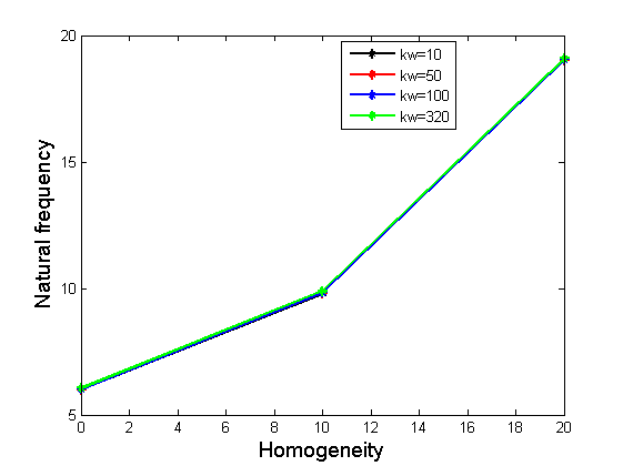
To consider the influence of the homogeneity on the fundamental natural frequency of the varying thickness rectangular plate, analysis is performed under different values of homogenous parameters adopted which are: $α = 0$ and $20$ , Taper parameter is assigned zero value to avoid interference of results. From the results obtained and illustrated in Table 6, it is observed that increases homogeneity increase the natural frequency of the rectangular plate under clamped condition. This implies that, as the material properties are being increased, the plates gained more stiffness. The more the plate get stiffened the more it becomes rigid and the natural frequency increases due to increase in stiffness of the plate as a result of increase homogeneity. Tables 5 and 6 also show that, the behavior is general to combine foundations parameter. Figure 4 and 5 illustrate the relationship between homogeneity and natural frequency of combine elastic foundations under clamped support condition.

Figure 4 Influence of homogeneity on natural frequency clamped edge condition

Figure 5 Influence of combine elastic foundations on natural frequency clamped edge condition

Figure 6 Influence of combine elastic foundations on nonlinear natural frequency

Table 7 Influence of homogeneity on fundamental natural frequency of shear Pasternak foundation
Edge Condition	Homogeneity	Natural frequencies $Ω$
		Taper $β = 0$ , $k_{w} = 0$
		$K_{s}$ =0,	$K_{s}$ =10	$K_{s}$ =50	$K_{s}$ =100	$k_{s}$ = 320
Clamped Support	$α$ =0	5.9936	5.9936	5.9936	5.9936	5.9936
	$α$ =10	9.7981	9.7981	9.7981	9.7981	9.7981
	$α$ =20	19.0158	19.0158	19.0158	19.0158	19.0158

The observation is justified with the underlined mathematical representation. $\begin{matrix} (77) & \begin{aligned} n a t u r a l f r e q . = \frac{ω a^{2}}{π^{2}} \sqrt{\frac{ρ h}{D}} \end{aligned} \end{matrix}$ where density is $ρ$ , $D$ is the flexural rigidity, $h$ is the thickness and $Ω$ is the natural frequency.

Tables 8 and 9 illustrate the influence of the taper variation on the natural frequency. Increase in taper ratio along $x$ -direction of the rectangular plates, means that as the thickness of the plate increase, the plate gain more strength and stiffness. The more the stiffness of the plate, the more that natural frequency of the plate increase. This is an obvious result considering the classical theory of vibration. Figure 7 and 8 show the graphical relationship between the taper increase and the natural frequency of the rectangular plate. This increase is significant based on the results obtained. The negative value of the taper assigned in the Figure 7 and 8 show reduction in the tapering of the plate while the positive values indicate that the thickness are increasing which is shown from zero upward in the graphical illustration respectively. The thread of results is observed for both combine case of foundations and when only elastic Winkler foundation is adopted.

Table 8 Influence of taper on natural frequency of combine foundations parameter coefficients
Edge Condition	Taper	Natural frequencies $Ω$
Edge Condition	Taper	Homogeneity $α_{1} = 0$
		$K_{s}$ =5, $K_{w}$ =10	$K_{s}$ =10, $K_{w}$ =50	$K_{s}$ =30, $K_{w}$ =100	$K_{s}$ =50, $K_{w}$ =320
Clamped Support	$β$ =-0.5	32.3922 +47.773 I	32.3926 +47.7722 I	32.3933+ 47.7713 I	32.3960+ 47.7674 I
	$β$ =0	5.9957	6.0040	6.0144	6.0600
	$β$ =0.5	27.7684 +15.176 I	27.7698 +15.1748	27.7716 +15.1739 I	27.7792 +15.1697 I
	$β$ =1.0	48.6564 +3.980 I	48.6571 +33.9797 I	48.6580 +33.9791 I	48.6618 +33.9765 I

Table 9 Influence of taper on natural frequency of combine foundations parameter coefficients
Edge Condition	Taper	Natural frequencies $Ω$
Edge Condition	Taper	Homogeneity $α_{1} = 0$ , $K_{w} = 0$
		$K_{s}$ =5	$K_{s}$ =10	$K_{s}$ =50	$K_{s}$ =100
Clamped Support	$β$ =-0.5	32.39203096 +47.77308213 I	32.39203069 +47.77308243 I	32.39203084 +47.77308223 I	32.39203086 +47.77308211 I
	$β$ =0	5.993625349	5.993625295	5.993624786	5.993624932
	$β$ =0.5	27.76809403 +15.17574761 I	27.76809412 +15.17574752 I	27.76809395 +15.17574771 I	27.76809358 +15.17574839 I
	$β$ =1.0	48.65620909 +33.98026006 I	48.65620904 +33.98025987 I	48.65620904 +33.98025999 I	48.65620895 +33.98026011 I

Figure 7 Influence of taper variation on natural frequency clamped edge condition

Figure 8 Influence of taper variation on combine elastic foundations on natural frequency clamped edge condition

Figure 9 Effects of non-homogeneity of the plate for the nonlinear analysis

Figure 10 Influence of thickness variation on nonlinear natural frequency

Figure 11 Influence of Aspect ratio variation on nonlinear natural frequency

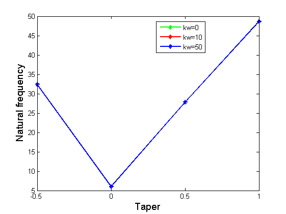
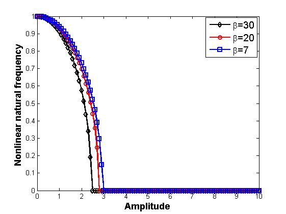
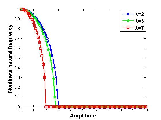
Figure 9 presents the variation on the nonlinear amplitude frequency curve response of the non-uniform rectangular plate. It is observed that as the non-homogeneity values is insignificant with nonlinear natural frequency. The effects of taper parameters variation on the nonlinear amplitude frequency curve response of the rectangular plate are studied and presented in Figure 10. It can be seen that, the nonlinear frequency of the rectangular plate decreases with increase in taper values. Figure 11 illustrates the effect of aspect ratio variation on the nonlinear analysis of the rectangular plate. It is observed that nonlinear frequency of the rectangular plate decrease with the increase aspect ratio values. The aspect ratio has a significant effect on the nonlinear frequency amplitude curve of the plate. It is observed that, an increase in the plate aspect ratio makes the rectangular plate to become stiffer and consequently lowers the nonlinear natural frequency of the plate. Figure 11 shows that values of nonlinear natural frequency have a direct relationship with the aspect ratio values as a result of lowering the softening nonlinearity.

5. Conclusion

The free vibration dynamic behavior of thin rectangular plate resting on elastic Winkler and Pasternak foundation using two-dimensional DTM was investigated. The solutions obtained were validated with literature cited with very precise results. However, the solutions obtained were subsequently used to investigate influence of controlling parameters on elastic foundations. The following observations were recorded.

Increase in Winkler foundation leads to increase in natural frequency of the plate. Same increase was recorded in the case of combined Pasternak and Winkler foundations.
Increase in taper shows that the natural frequency increases.
Increase in non-homogeneity of the plate leads to natural frequency increases.
Nonlinear natural frequency ratio increases with increase in elastic foundation parameters.
Nonlinear natural frequency decreases with the increase in taper values.
It is observed that nonlinear natural frequency decreases with the increase of aspect ratio values.

The present study has revealed the importance of varying thickness, homogeneity on dynamic behaviour of rectangular plates.

Abbreviations: Nomenclature

$k_{w}$ : Linear Winkler foundation parameters

$k_{s}$ : Shear modulus of Pasternak foundation

$\frac{d}{d x}$ : Differential operator

$w$ : transverse deflection

$a, b$ : Dimension of rectangular plate

References

Kang, J. H. (2003). Three-dimensional vibration analysis of thick, circular and annular plates with nonlinear thickness variation. Computers & structures, 81(16), 1663-1675.
Sharma, S., Gupta, U. S., & Singhal, P. (2012). Vibration analysis of non-homogeneous orthotropic rectangular plates of variable thickness resting on Winkler foundation. Journal of Applied Science and Engineering, 15(3), 291-300.
Bahmyari, J.E., & Rahbar-Ranji, A. (2012). Free Vibration of Orthropic Plates with Variable thicjness resting on non-uniform elastc foundation by elment free Galerking method. Journal of Mechanical Science and Technology, 26(9), 2685-2694.
Leissa, A. W. (1987). Recent studies in plate vibrations: 1981-1985. Part 2: Complicating effects. Vibration Inst., The Shock and Vibration Digest, 19(3), 10-24.
Leissa, A. (1980). Plate vibration research, 1976-1980: complicating effects. Shock and Vibration Inform. Center the Shock and Vibration Digest, 13(10), 19-36.
Leissa, A.W. (1987). Recent Studies in Plate Vibration. Part 1: Classical Theory. The shock and Vibration digest, 19, 11-18.
Leissa, A. W. (1969). Vibration of plates, Vol. SP-160. NASA, Washington, DC: US Government Printing Office.
Sakiyama, T., & Huang, M. (1998). Free vibration analysis of rectangular plates with variable thickness. Journal of Sound and Vibration, 216(3), 379-397.
Amini, M. H., Soleimani, M., & Rastgoo, A. (2009). Three-dimensional free vibration analysis of functionally graded material plates resting on an elastic foundation. Smart Materials and Structures, 18(8), 1-9.
Semnani, S. J., Attarnejad, R., & Firouzjaei, R. K. (2013). Free vibration analysis of variable thickness thin plates by two-dimensional differential transform method. Acta Mechanica, 224(8), 1643-1658.
Chakraverty, S. (2008). Vibration of plates. CRC press.
Matsuda, H., & Sakiyama, T. (1987). Bending Anaysisof rectangular plate nonuniform thickness resting on elastic foundation. Japan society of civil engineering struct eng/earthquake, 4(1), 51-59.
Miandoab, E.M, Tajaddodianfar, F., Pishkenari, H.N., & Ouakad, N.M. (2015). Analytical solution for forced vibration of a nano resonantor with cubic nonlinear using Homotopy Analysis method. Int. J nanosci, Nanotechnology, vol. 2(3), 159-160.
Ranji, A. R., & Hoseynabadi, H. R. (2010). A semi-analytical solution for forced vibrations response of rectangular orthotropic plates with various boundary conditions. Journal of Mechanical Science and Technology, 24(1), 357-364.
Sobamowo, M. G. (2018). Combine effects of thermal radiation and nanoparticles on free convection flow and heat transfer of casson fluid over a vertical pate. Int. Journal of chemical engineering. Hindawi, 2018, 1-25.
Ogunjiofor, E. I. & Nwoji, C. U. (2017).Analytical Bending Solution of all Clamped Isotropic Rectangular Plate on Winkler Foundation using Characteristic Orthogonal Polynomial. Nigerian Journal of Technology, 36(3), 724-728.
Zhou, J. K. (1986). Differential Transformation and its applications for electrical circuits, Huazhong univ. Press, wuhan, China.
Chen, C. O. K. & Ho, S. H. (1999). Solving partial differential equations by two-dimensional differential transform method. Applied Mathematics and computation, 106(2-3), 171-179.
Ayaz, F. (2003). On two-dimensional differential transform method. Applied Mathematics and computation, 143, 36-374.
Selvadurai, A. P. (2013). Elastic analysis of soil-foundation interaction. Elsevier.
Weidenhammer, F. (1973). L. Fr $\overset{´}{y}$ ba, Vibration of Solids and Structures under Moving Loads. Czechoslovak Academy of Sciences. Zeitschrift Angewandte Mathematik und Mechanik, 53, 502-503.
Semnani, S. J., Attarnejad, R. & Firouzjaei, R. K. (2013). Free vibration analysis of variable thickness thin plates by two-dimensional differential transform method. Acta Mechanica, 224(8), 1643-1658.
Sakata, T. (1977). Forced vibrations of a rectangular plate with non-uniform thickness. Journal of Sound and Vibration, 53(1), 147-152.
Gupta, A. K., Saini, M., Singh, S. & Kumar, R. (2014). Forced vibrations of non-homogeneous rectangular plate of linearly varying thickness. Journal of Vibration and Control, 20(6), 876-884.
Rao, J. S. (1999). Dynamics of plates. Alpha Science Int’l Ltd.

Contents