This study focused on line integral and its applications. The study was designed to show the areas where line integral is applicable and point out the role of line integral in solving practical problems. The study found out that space curves, and the concepts of scalar and vector fields are basic concepts to deal line integral. Also, the study found out that line integral is used to calculate mass, center of mass and moments of inertia of a wire, work done by a force on an object moving in a vector field, magnetic field around a conduct, voltage generated in a loop, length of a curve, area of a region bounded by a closed curve, and volume of a solid formed by rotating a closed curve about the \(x-\)axis.
In mathematics, a line integral is an integral where the function to be integrated is evaluated along a curve. The terms path integral, curve integral, and curvilinear integral are also used; contour integral as well, although that is typically reserved for line integral in the complex plane [1].
The function to be integrated may be a scalar field or a vector field. The value of the line integral is the sum of values of the field at all points on the curve, weighted by some scalar function on the curve (commonly arc length) or, for a vector field, the scalar product of the vector field with a differential vector in the curve. This weighting distinguishes the line integral from simpler integrals defined on intervals. Many simple formula in physics (for example, \(W = F \cdot s\)) have natural continuous analogs in terms of line integrals ( \(W = \int_{c}F~\cdot~ ds\)). The line integral finds the work done on an object moving through an electric or gravitational field, for example [1].
The main purposes of this study are to
Definition 1.(Vector valued function [2]) A function \(r : t\longrightarrow\mathbf{V}\) is said to be a vector valued function if \(t \in ~\mathbb{R}\) and \(\mathbf{V}\) is \(n-\)dimensional vector.
Example 1. \(r(t) = 2ti-t^{2}j\) and \(r(t) = i-tj + (\sin t)k\) for any real number \(t\) are vector valued functions.
Definition 2.(Space curve [2]) A space curve (or simply curve) is the range of a continuous vector valued function on an interval of real numbers.
We will generally use \(C\) to denote a curve and \(r\) to denote a vector valued function whose range is a curve \(C.\) In that case we say that \(C\) is parameterized by \(r\) or that \(r\) is a parametrization of \(C.\)There are so many types of curves. Some of them are listed as follows;
Definition 3.(Simple curve [3]) A curve \(C\) is said to be simple if it has no self-intersection except possibly at the end points of the interval of a parameter \(t.\)

Definition 4.(Closed curve [3]) A curve \(C\) is said to be closed if it has a parametrization \(r(t)\) on the closed interval \([a, b]\) such that \(r(a) = r(b).\) In other words, a curve \(C\) is said to be closed if its initial and terminal points coincides.
Example 2.
Definition 5.(Simple closed curve [3]) A curve \(C\) is said to be simple closed if it is both simple and closed curve.
Definition 6.(Smooth curve [3]) A vector valued function \(r(t)\) is said to be smooth on an interval \(I\) if \(r'(t)\) is continuous on \(I\) and \(r'(t) \neq 0\) for each interior point of \(I.\) A curve \(C\) is said to be smooth if its parametrization \(r(t)\) is smooth.
Example 3.
Definition 7.(Piecewise smooth curve [3]) A vector valued function \(r(t)\) is said to be piecewise smooth on an interval \(I\) if \(I\) is expressible as the union of finite number of subintervals such that \(r(t)\) is smooth on each of the subintervals and the one-sided derivatives of \(r(t)\) exist at each interior point of \(I.\) A curve \(C\) is said to be piecewise smooth if its parametrization \(r(t)\) is a piecewise smooth.
For 2 in Example 3, \(r(t)\) is piecewise smooth because \(r(t)\) is smooth on subintervals \([-2\pi, 0]\) and \([0, 2\pi]\), and one-sided derivatives of \(r(t)\) exist on \((-2\pi,~2\pi).\) Because of this, that curve is a piecewise smooth on \([-2\pi,~2\pi].\)
Remark 1. Any smooth curve can be piecewise smooth but the converse is not always true.
Definition 8.(Counter clockwise oriented curve [4]) A curve \(C\) is said to be counter clockwise oriented if it is always lying to the left of the path while moving along \(C.\)
Definition 9. (Clockwise oriented curve [4]) A curve \(C\) is said to be clockwise oriented if it is always lying to the right of the path while moving along \(C.\)
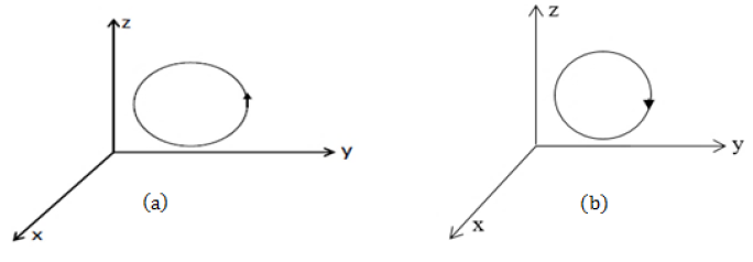
Definition 10. (Positively and Negatively oriented curves [4])
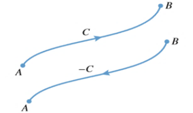
Remark 2. If the curve is simple closed, then it is
It is possible to express different curves using a parameter. Now, let us see smooth parametrization of important curves which we will use frequently.
Line segment: Suppose \(L\) is a line segment from point \(A(x_{0},~y_{0},~z_{0})\) to another point \(B(x_{1},~y_{1},~z_{1})\). Then the parametric equation of this line segment is
\[ \begin{cases} x=x_{0} + (x_{1}- x_{0})t \\ y=y_{0}+(y_{1}-y_{0})t\\ z=z_{0}+(z_{1}-z_{0})t \end{cases}\] for \(0\leq t\leq 1.\) Therefore, the smooth parametrization of this line segment is \[[x_{0}+(x_{1}-x_{0})t]i +[y_{0}+(y_{1}-y_{0} )t]j+[z_{0}+(z_{1}-z_{0})t]k\;\;\;\;\;\;\; \text{for }\;\;\;\;\;\;0\leq t\leq 1.\]Circle: Suppose \(C\) is a circle with equation \((x-h)^{2}+(y-k)^{2}=r^{2}\). Then the parametric equation of this circle is
\[ \begin{cases} x=h+r\cos t \\ y=k+r\sin t \end{cases}\] for \(0\leq t\leq 2\pi. \) Therefore, the smooth parametrization of this circle is \[[h+rcost]i+[k+r\sin t]j\;\;\;\;\;\;\; \text{for }\;\;\;\;\;\;0\leq t\leq 2\pi.\]Ellipse: Suppose \(E\) is an ellipse with equation \(\frac{(x-h)^{2}}{a^{2}} +\frac{(y-k)^{2}}{b^{2}} =1\). Then the parametric equation of this ellipse is
\[\begin{cases} x=h+a\cos t \\ y=k+b\sin t \end{cases}\] for \(0\leq t\leq 2\pi. \) Therefore, the smooth parametrization of this ellipse is \[[h+acost]i+[k+b\sin t]j\;\;\;\;\;\;\; \text{for }\;\;\;\;\;\;0\leq t\leq 2\pi.\]Graph of a function: Suppose \(C\) is a graph of a function \(y = g(x)\) for \(a\leq x \leq b\). Then the parametric equation of this graph is
\[\begin{cases} x=t\\ y=g(t) \end{cases} \] for \(a\leq t\leq b. \) Therefore, the smooth parametrization of this graph is \[ti+g(t)j \;\;\;\;\;\;\; \text{for }\;\;\;\;\;\;a\leq t\leq b.\]Region formed by a plane \(z = m\) and a circle \((x-h)^{2}+(y-k)^{2}=r^{2}\): The smooth parametrization of this region is
\[[h+r\cos t]i+[ k+r\sin t]j+mk\;\;\;\;\;\;\; \text{for }\;\;\;\;\;\;0\leq t \leq 2\pi.\]Sphere: Suppose \(S\) is a sphere with equation \((x-h)^{2} + (y-k)^{2} + (z-w)^{2} =\rho^{2}\). Then the parametric equation of this sphere is
\[ \begin{cases} x=h+\rho \cos\beta \sin\theta \\ y=k+\rho \sin\beta \sin\theta\\ z=w+\rho \cos\theta \end{cases} \] for \(\beta \in [0,~ 2\pi]~and~\theta \in [0,~ \pi] \). Therefore, the smooth parametrization of this sphere is \[[h+\rho \cos\beta \sin\theta]i+[k+\rho \sin\beta \sin\theta]j +[w+\rho \cos\theta] k\;\;\;\;\;\;\; \text{for }\;\;\;\;\;\;\beta \in [0,~ 2\pi]~and~\theta \in [0,~ \pi].\]Definition 11. (Length of a curve [2]) Let \(C\) be a curve with a piecewise smooth parametrization \(r(t)\) defined on \([a, b],\) then the length \(L\) of \(C\) is \begin{equation*} L=\int_{a}^{b}|r'(t)|dt=\int_{a}^{b}|\frac{dr}{dt}|dt. \end{equation*}
Remark 3.If \(r(t) = x(t)i + y(t)j + z(t)k,\) then \begin{equation*} L=\int_{a}^{b}\sqrt{[x'(t)]^{2}+[y'(t)]^{2}+[z'(t)]^{2} }dt. \end{equation*}
Example 4. Consider a curve parameterized by \(r(t) = (\cos t)i + (\sin t)j + tk\) for \(0\leq t \leq 2\pi\). The derivative of \(r(t)\) with respect to \(t\) is \begin{equation*} r'(t)=(-\sin t)i+(\cos t )j+k. \end{equation*} The length of this curve on \([0, 2\pi]\) is \begin{equation*} L=\int_{0}^{2\pi}\sqrt{(-\sin t)^{2}+(\cos t)^{2}+1^{2}} dt =\int_{0}^{2\pi}\sqrt{2}dt=2\sqrt{2}\pi. \end{equation*}
Definition 12. (Scalar field [3]) A function \(f : P\rightarrow Q\) is said to be a scalar field if \(P\in\mathbb{R}^{n}\) and \(Q\in\mathbb{R}\).
Example 5. \(f(x, y, z) = xyz\) is a scalar field.
Definition 13. (Vector field [3]) A function\( F : P\rightarrow\mathbf{V}\) is said to be a vector field if \(P\in\mathbb{R}^{n}\) and \(\mathbf{V}\) is \(n-\)dimensional vector.
Example 6. \(F(x, y, z) = x^{2} i+y^{2} j+z^{2} k\) is a vector field.
Remark 4.A vector field \(F\) formed by the gradient of a scalar function \(f\) is said to be gradient vector field and denoted by \begin{equation*} F = \triangledown f=(\frac{\partial}{\partial x}i + \frac{\partial}{\partial y}j + \frac{\partial }{\partial z}k)f=f_{x}i+f_{y}j+f_{z}k. \end{equation*}
Definition 14. (Conservative vector field [3]) A vector field \(F\) is said to be conservative if there exists a differentiable function \(f\) such that \(F = \triangledown f.\) The function \(f\) is called potential function for \(F.\)
Example 7. A function \(F(x, y, z) = 3x^{2} i+3y^{2} j+3z^{2}k\) is conservative because there exists a potential function \(f(x, y, z) = x^{3} +y^{3}+z^{3}\) for \(F\) such that \(F = \triangledown f.\)
Before we see test of conservativeness, let us define the curl of a vector field \(F.\)Definition 15. (Curl of a vector field [3]) Let \(F = Mi + Nj + Pk\) be a vector field such that all the partial derivatives of \(M, N\) and \(P\) exist, then the curl of \(F,\) denoted by curl \(F,\) is given by \[\text{curl}~F=\triangledown \times F = \begin{vmatrix} i & j & k \\ \frac{\partial}{\partial x} & \frac{\partial }{\partial y} & \frac{\partial }{\partial z} \\ M & N & P \end{vmatrix} .\]
Remark 5. If \(F = Mi +Nj,\) then \(\text{curl} F = (N_{x}-M_{y})k\).
Example 8. Consider a vector field \(F(x, y, z) = 3x^{2}i + xyj – y^{2}zk\). Then the curl of \(F\) is given by \[ \begin{vmatrix} i & j & k \\ \frac{\partial }{\partial x} & \frac{\partial }{\partial y} & \frac{\partial }{\partial z} \\ 3x^{2} & xy & -y^{2} z \end{vmatrix} = -2yzi + yk.\]
Now let us see test of conservativeness and procedures of finding potential function of conservative vector field.Step-1 ( Variable separation) In this step, we express the function \(f\) as a sum of three functions in the form of \[f(x,~y,~z)=k(x,~y,~z)+g(y,~z)+h(z).\] So, \(f_{x}=k_{x},~f_{y}=k_{y}+g_{y}\) and \(f_{z}=k_{z}+g_{z}+h_z.\) Since \(F = \triangledown f,\) then \(f_{x}=k_{x}=M,~f_{y}=k_{y}+g_{y}=N\) and \(f_{z}=k_{z}+g_{z}+h_{z}=P\).
Step-2 Integrate \(f_{x}=k_{x}=M\) with respect to \(x.\) That is \(k(x, y, z)\) = \(\int Mdx\).
Step-3 Integrate \(f_{y}=k_{y}+g_{y}=N\) with respect to \(y.\) That is \(g(y,z)=\int(N-k_{y})dy\).
Step-4 Integrate \(f_{z}=k_{z}+g_{z}+h_{z}=P\) with respect to \(z.\) That is \(h(z)=\int(P-k_{z}-g_{z})dz\).
Step-5 Finally, we write \(f(x, y, z) = k(x, y, z) + g(y, z) + h(z)\) using the above results.
Example 9. Consider a vector field \(F(x, y, z)= xy^{2}z^{2} i+x^{2} y z^{2} j+x^{2} y^{2} zk\). Then \( M=x y^{2} z^{2},~ N=x^{2} y z^{2}\) and \(P=x^{2} y^{2} z\).
Firstly, let us test \(F\) is conservative or not. \[ \text{curl} F = \begin{vmatrix} i & j & k \\ \frac{\partial }{\partial x} & \frac{\partial }{\partial y} & \frac{\partial }{\partial z} \\ xy^{2}z^{2} & x^{2} y z^{2} &x^{2} y^{2} z \end{vmatrix} = 0.\] Hence, this vector field is conservative.Definition 16.(Line integral of scalar field [3]) Let \(f\) be a continuous scalar field on a smooth curve \(C\) parameterized by \(r(t) = x(t)i + y(t)j + z(t)k\) on \([a, b],\) then the line integral of \(f\) on \(C\) is given by \begin{equation*} \int_{C} f(x,y,z)ds = \int_{a}^{b}f(x(t),~y(t),~z(t)) |r'(t)|dt. \end{equation*}
Example 10.
Definition 17.(Line integral of vector field [3]) Let \(F = Mi + Nj + Pk\) be a continuous vector field defined on a smooth curve \(C\) parameterized by \(r(t) = x(t)i + y(t)j + z(t)k\) on \([a, b],\) then the line integral of \(F\) on \(C\) is given by \[ \int_{C} F\cdot dr=\int_{a}^{b} F(x(t),~y(t),~z(t)) \cdot r'(t)dt.\]
Example 11. Consider \(F(x, y) = 3yi + 3xj\) and \(C\) is the ellipse \(\frac{x^{2}}{9}+\frac{y^{2}}{4}=1\) in the \(xy-\)plane. The smooth parametrization of this ellipse is \[r(t) = (3\cos t)i + (2\sin t)j; \;\;\;\;\;\;0\leq t \leq 2\pi\,,\] implies \[F(x(t),y(t))\cdot r'(t)=[(6\sin t)i +(9\cos t)j]\cdot [(-3\sin t)i +(2\cos t)j]=18\cos 2t.\] Hence, the line integral of \(F\) on \(C\) is \( \int_{C} F(x,y)\cdot dr=\int_{o}^{2\pi}(18 \cos 2t) dt=0\).
Remark 6. If \(a\) and \(b\) are constants, and \(F\) and \(G\) are continuous vector field on a smooth curve \(C\) parameterized by \(r(t),\) then the following properties hold;
Example 12.
Consider \(F(x, y) = xi + yj \) and \( C\) is the triangle in a plane with vertices \(A(0, 0), B(1, 0)\) and \( C(0, 1)\) in counter clockwise orientation, see Figure 4.
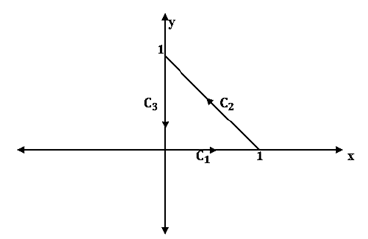
From Figure 4, \(C = C_{1} ~\bigcup ~C_{2} ~\bigcup~ C_{3}\), where \(C_{1}:x=t\) and \(y = 0; \;\;\;\;0\leq t \leq 1\), \(C_{2}:x=1-t\) and \(y = t;\;\;\;\;0\leq t \leq 1\), and \(C_{3}:x=o\) and \(y = 1\;\;t;\;\;\;\;0\leq t\leq 1\).
On \(C_{1},\) \[\int_{C_{1} } F\cdot dr=\int_{0}^{1}t dt=\frac{1}{2}.\] On \(C_{2},\) \[\int_{C_{2}} F\cdot dr=\int_{0}^{1}(2t-1) dt=0.\] On \(C_{3},\) \[\int_{C_{3 }} F\cdot dr=\int_{0}^{1}(t-1)dt=-\frac{1}{2}.\] Hence, \[\int_{C} F\cdot dr=\int_{C_{1 }} F\cdot dr+\int_{C_{2 }} F\cdot dr+ \int_{C_{3 }} F\cdot dr=\frac{1}{2}+0-\frac{1}{2}=0.\] In other way, since \(F\) is conservative, \( f(x, y) = \frac{x^{2}}{2}+\frac{y^{2}}{2}\) is a potential function for \(F\) and \( C\) is closed path, then \(\int_{C} F\cdot dr=f(0,0)-f(0,0)=0\).Definition 18.(Contour integral [5]) If a function of complex variable \(f(z)\) is continuous on a smooth curve \(C\) parameterized by \(z(t) = x(t) + y(t)i\) on an interval \([a, b],\) then the contour integral of \(f\) on \(C\) is given by \[\int_{C} f(z)dz=\int_{a}^{b}f(z(t)) z'(t)dt.\]
Remark 7. Contour integral grants all properties of line integral in Cartesian plane.
Example 13. Consider \(f(z) = z^{2}\) and \(C\) is given by Figure 5.
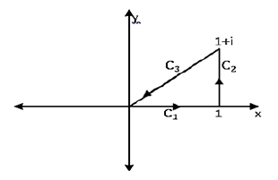
From Figure 5, \(C = C_{1} ~\bigcup ~C_{2} ~\bigcup~ C_{3}\), wehere \(C_{1} : z(t) = t; \;\;\;0\leq t\leq 1\), \(C_{2}: z(t) = 1+ti; \;\;\;0\leq t\leq 1\) and \(C_{3}: z(t) = (1-t) + (1-t)i; \;\;\;0\leq t\leq 1\).
On \(C_{1},\) \[ \int_{C_{1 }} f(z)dz=\int_{0}^{1}t^{2} dt=\frac{1}{3}.\] On \(C_{2},\) \[\int_{C_{2 }} f(z)dz=\int_{0}^{1}(1+ti)^{2 }i dt=-1+\frac{2}{3} i.\] On \(C_{3},\) \[\int_{C_{3 }} f(z)dz=\int_{0}^{1}[(1-t)+(1-t)i]^{2} (-1-i)dt=\frac{2}{3}-\frac{2}{3} i.\] Hence, \[\int_{C} f(z)dz=\int_{C_{1 }} f(z)dz+\int_{C_{2}} f(z)dz+ \int_{C_{3}} f(z)dz=0.\]If the curve \(C\) is two-dimensional, the latter formula can be written in the form of
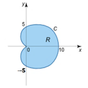
\begin{equation*} L=\int_{C} ds=\int_{\alpha}^{\beta}|\frac{dr}{dt}| dt = \int_{\alpha}^{\beta} \sqrt{(\frac{dx}{dt})^{2}+(\frac{dy}{dt})^{2}} ~dt. \end{equation*} If the curve \(C\) is the graph of a continuous and differentiable function \(y = f(x)\) on \([a, b]\) in the \(xy-\)plane, then the length of the curve is given by \begin{equation*} L=\int_{a}^{b}\sqrt{1+(\frac{dy}{dx})^{2}} ~dx. \end{equation*} Finally, if the curve \(C\) is given by the equation \(r = r(\theta ),\) \(\alpha \leq \theta \leq \beta\) in polar coordinates, and the function \(r(\theta)\) is continuous and differentiable in the interval \([\alpha, \beta],\) then the length of the curve is defined by the formula \begin{equation*} L=\int_{\alpha}^{\beta}\sqrt{(\frac{dr}{d\theta})^{2}+r^{2}}~ d\theta. \end{equation*}Example 14.
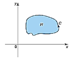
Remark 8. It is supposed here that the contour \(C\) is traversed in the counterclockwise direction.
If the closed curve \(C\) is given in parametric form \(r(t) = (x(t), y(t))\) on \([\alpha,~ \beta],\) then the area of the corresponding region can be calculated by the formula \begin{equation*}S=\int_{\alpha}^{\beta}x(t) \frac{dy}{dt} dt=-\int_{\alpha}^{\beta}y(t) \frac{dx}{dt} dt=\frac{1}{2} \int_{\alpha}^{\beta}[x(t) \frac{dy}{dt}-y(t) \frac{dx}{dt}]dt \,. \end{equation*} Example 15. Consider a region bounded by the ellipse \(x = a\cos t, y = b\sin t; \;\;\;0\leq t \leq 2\pi\), see Figure 8.
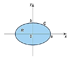
The area of this region is
\begin{equation*} S=\int_{0}^{2\pi}(a\cos t) (b\cos t)dt=ab\int_{0}^{2\pi}\cos^{2} tdt=\pi ab. \end{equation*}We can also get the following result using the other two formulas;
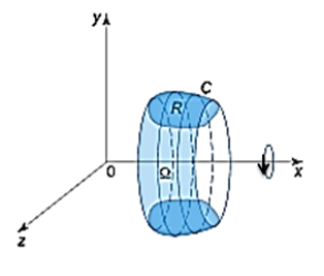
Example 16. Consider a solid formed by rotating the region \(R\) bounded by the curve \(y = 2-\sin x\) and the lines \(x = 0, x = 2\pi, y = 0\) about the \(x-\)axis (Figure 10).
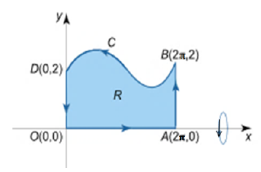
The volume of the solid is
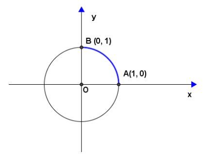
\begin{align*} V&=-\pi \oint_{C} y^{2} dx=-\pi [\int_{OA} y^{2} dx+\int_{AB} y^{2} dx+\int_{BD} y^{2} dx+\int_{DO} y^{2} dx]\\ &=-\pi(0+0-9\pi+0)=9\pi^{2} \end{align*} where, since \(y = 0\) on \(OA\), so \(\int_{OA} y^{2} dx=\int_{0}^{2\pi}o^{2} dx=0\). Since, the smooth parametrization of \(AB\) is \(2\pi i +2tj\), so \[\int_{AB} y^{2} dx=\int_{2\pi}^{2\pi}y^{2}dx=\int_{0}^{1}(2t)^{2}\times 0~ dt =0.\] Since \(y = 2- \sin x\) on \(BD\), so \[\int_{BD} y^{2} dx=\int_{2\pi}^{0}(2-sinx )^{2} dx=-9\pi.\] Since, the smooth parametrization of DO is \(0i + (2 \)-\( 2t)j\), so \[\int _{DO} y^{2} dx=\int_{0}^{0}y^{2} dx=\int_{0}^{1}(2-2t)^{2}\times 0 ~dt =0.\]Example 17. Consider a wire lying along the arc of the circle \(x^{2}+y^{2}=1\) from \(A(1, 0)\) to \(B(0, 1)\) with the density \(\rho(x, y) = xy\) (Figure 11).
Example 18. Consider a circle \(x^{2} + y^{2} = a^{2}\) with the density \(\rho\) = 1. The parametric equation of this circle is\[ \begin{cases} x=a\cos t \\ y=a\sin t \end{cases} \] for \(0 \leq t \leq 2\pi\). Then the moment of inertia \(I_{x}\) about the \(x-\)axis is \begin{equation*} I_{x}=\int_{0}^{2\pi}(a\sin t)^{2}\times 1\times \sqrt{(-a\sin t)^{2}+(a\cos t)^{2}} dt=a^{3} \int_{0}^{2\pi}\sin^{2}t dt = \pi a^{3}\,. \end{equation*}

Remark 9. The force field \(F\) is not necessarily the cause of moving the object. It might be some other force acting to overcome the force field that is actually moving the object. In this case the work of the force \(F\) could result in a negative value.
If a vector field is defined in the coordinate form \(F = (P(x, y, z), Q(x, y, z), R(x, y, z)),\) then the work done by the force is calculated by the formula
\begin{equation*} W=\int_{C} F ~. ~dr=\int_{C} [Pdx+Qdy+Rdz]. \end{equation*} If the object is moved along a curve \(C\) in the \(xy-\) plane, then the following formula is valid \begin{equation*} W=\int_{C} F~.~dr=\int_{C} [Pdx+Qdy] \end{equation*} where \(F = (P(x, y), Q(x, y)).\)If a path \(C\) is specified by a parameter \(t\) (\(t\) often means time), the formula for calculating work becomes
\begin{equation*} W = \int_{\alpha}^{\beta}[P(x(t),y(t),z(t)) \frac{dx}{dt} +Q(x(t),y(t),z(t)) \frac{dy}{dt}+R(x(t),y(t),z(t)) \frac{dz}{dt} ]dt\,, \end{equation*} where \(t\) goes from \(\alpha\) to \(\beta\). If a vector force field \(F\) is conservative, then the work on an object moving from \(A\) to \(B\) can be found by the formula \begin{equation*} W=u(B)-u(A)\,, \end{equation*} where \(u(x, y, z)\) is a scalar potential function of a vector force field \(F.\)Example 19. Consider a force field \(F(x, y) = (xy, x + y)\) on an object moving from the origin \(O(0, 0)\) to the point \(A(1, 1)\) along the path \(C.\)
Remark 10. For Example 19, if the force field is \(F(x, y) = xi + yj,\) then \(F\) is conservative force and in cases a and b, the work done is independent of the path i.e., \(W = f(1, 1)- f(0, 0) = 1\) where \(f(x, y) = \frac{x^{2}}{2} + \frac{y^{2}}{2} + c\) is a potential function for a force field \(F(x, y) = xi + yj.\)

Example 20. Let us develop the formula of the magnetic field in vacuum a distance \(r\) from the axis of a long straight wire carrying current \(I.\)
To find the field a distance \(r\) from the wire, we consider a loop of radius \(r,\) centered on the wire with its plane perpendicular to the wire with the current \(I\) (Figure 14). Since the field \(B\) has a constant magnitude and the field is tangent to the loop everywhere, the dot product of the vectors \(B\) and \(dr\) is just \(Bdr.\) Then we can write \begin{equation*} \oint_{C} B~.~dr=\oint_{C} Bdr=B\oint_{C} dr=B\int_{0}^{2\pi}dr=2\pi rB\,. \end{equation*} As a result, we have \(2\pi rB=\mu_{0} I \Longrightarrow B=\frac{\mu_{0} I}{2\pi r}\).
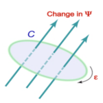
Example 21. Let us evaluate the maximum electromotive force \(\epsilon\) and the electric field \(E\) induced in a finger ring of radius \(1cm\) when the passenger flies on an airplane in the magnetic field of the Earth with the velocity of \(900km/h.\)
According to Faraday\(‘\)s law, \begin{equation*} \epsilon=\oint_{C} E~.~dr=-\frac{d\psi}{ dt}\,. \end{equation*} As the conducting ring moves through the Earth magnetic field, there is a change in the magnetic flux \(\psi\), passing through the ring. Suppose that the magnetic field \(B\) is perpendicular to the plane of the ring. Then change in the flux for the time \(\vartriangle t\) is \begin{equation*} \vartriangle \psi=2rBx=2rBv\vartriangle t\,, \end{equation*} where \(x = v\vartriangle t, v\) is the velocity of the airplane and \(B\) is the magnetic field of the Earth. It follows from the last expression that \begin{equation*} \epsilon=-\frac{d\psi}{dt}=2rBv. \end{equation*} Substituting the given values \( v = 900km/h = 250m/s, r = 1cm = 0.01m\) and \(B = 5\times10^{-5} T\), we obtain the electromotive force \( \epsilon=2rBv=2 \times 0.01 \times 5\times 10^{-5} \times 250=0.00025V\). As it can be seen, it’s safe for human.We can find the electric field in the conducting ring by the formula \(\epsilon=\oint_{C} E~.~dr\).
By symmetry, the induced electric field will have a constant magnitude along the ring. Its direction will be tangential to the circle at every point. Hence, the line integral around the circle is
\begin{equation*} \epsilon=\oint_{C} E~.~dr=\oint_{C} Edrcos0=E\oint_{C} dr=2\pi rE\,. \end{equation*} Hence, the electric field strength is \begin{equation*} E=\frac{\epsilon}{2\pi r}=\frac{0.00025}{2\pi \times 0.01}=0.00398V/m. \end{equation*}Acknowledgments First of all, I would like to thank my colleagues at Debark University for giving me their genuine advices and constructive comments from the very beginning of this study till its end. Secondly, my thanks also go to department of Mathematics, Debark University, which helped me in copying available hard materials and printing available soft copy materials for this study. Finally, I am deeply indebted to my wife Manayesh Melkamu for her encouragement to do this study and I would like to say God bless her.