In this paper, we formulate a new seven-step algorithm using a modified new iterative method for the numerical solution of the nonlinear gas dynamics equation. Three test cases are considered to demonstrate the feasibility and efficiency of the proposed method. Furthermore, numerical solutions show a good agreement with analytical solutions and some available examples from the available literature.
Gas dynamics is the science of the flow of air and other gas and or the notion of bodies through the air and other gas and its effects on physical systems, fluid mechanics, and thermodynamics; this science considers the products of combustion and combustion. The equations of gas dynamics are mathematical expressions based on the natural laws of conservations (mass, momentum, and energy). The study of shock fronts, rare fractions, and contact discontinuities are three major nonlinear wave equations that describe ideal gas dynamics behaviors [1]. Gas dynamics is synonymous with aerodynamics when the gas field is air, and the subject of study is flight. This is a core interest in aircraft and spacecraft design with their respective propulsion systems. Study in gas dynamics coincides with the developments of transonic and supersonic flight as the aircraft began to travel faster, and the density of air began to change, considerably increasing the air resistance as the airspeed approached the speed of sound. This phenomenon was later identified in wind tunnel experiments as an effect caused by the formation of shock waves around the aircraft. Major advances were made to describe the behavior during and after World War II, and the new understandings of compressible and high-speed flows became theories of gas dynamics [2].
In this paper, we consider nonlinear gas dynamic equation in one spatial dimension of the form:
In this paper, we construct a seven-step algorithm based on the modified new iterative method (MNIM) without using any transformation, linearization, and discretization for solving nonlinear gas-dynamic equation.
Consider the new iterative method (NIM) as a numerical technique for solving an functional equation of the form
Algorithm 1. restart:
Step 1:
Digits:=35;
\(N:=R^{+};\)
\(\tau:=R^{+};\)
\(\psi\left(x,t_0\right):=h(x);\)
\(\psi\left[0\right]:=\psi (x,t_0);\)
Step 2:
\(GDPDE:=value(-\tau*\psi*diff(\psi[0],x)-\psi*(1-\psi)+g(x,t));\)
\(\psi\left[1\right]:=value(int(GDPDE,t=0…t));\)
Step 3:
for p from 1 to N do
\(\psi\left[p+1\right]:=value((int(((-\tau*(sum(\psi[n],n=0…p))*Diff(sum[n],n=0…p,x)-(sum(\psi[n],n=0…p))*\)
\((1-sum(\psi[n],n=0…p))+g(x,t))))-(int(((-\tau*(sum(\psi[n],n= 0…p-1))*Diff(sum(\psi[n],n=0…p-1,x)-(sum(\psi[n],n=0…p-1))*(1-sum(\psi[n],n=0…p-1))+g(x,t)))));\)
end do
Step 4:
\(Example:=evalf(sum(\psi[k],k=0…N+1))\)
Step 5:         (11)
for i from 0 by 0.2 to 1 do\(\psi\left[i\right]:=evalf(eval(Example,[x=0.001,t=i]))\)
end do
Step 6:
for i from 0 by 2 to 10 do
\(N\left[0\right]:=evalExample,[x=0]);\)
\(N\left[2\right]:=eval(Example,[x=2]);\)
\(N\left[4\right]:=eval(Example,[x=4]);\)
\(N\left[6\right]:=eval(Example,[x=6]);\)
\(N\left[8\right]:=eval(Example,[x=8]);\)
\(N\left[10\right]:=eval(Example,[x=10]);\)
end do
Step 7:
\(\psi\left[3Dplot\right]:=plot3d(Example,t=-\pi…\pi,x=-\pi…\pi,grid=[100,100],color);\)
\(\psi\left[2Dplot\right]:=plot([N[0],N[2],N[4],N[6],N[8],N[10]]),t=0…40,color\)
=[red,blue,green,yellow,black,purple],axes=BOXED,title=GDPDE);
\(\psi\left[2Dlogplot\right]:=logplot([N[0],N[2],N[4],N[6],N[8],N[10]]),t=0…40,color\)
=[red,blue,green,yellow,black,purple],axes=BOXED,title=GDPDE);
\(\psi\left[Densityplot\right]:=(Example,t=-100…100,x=0…-10);\)
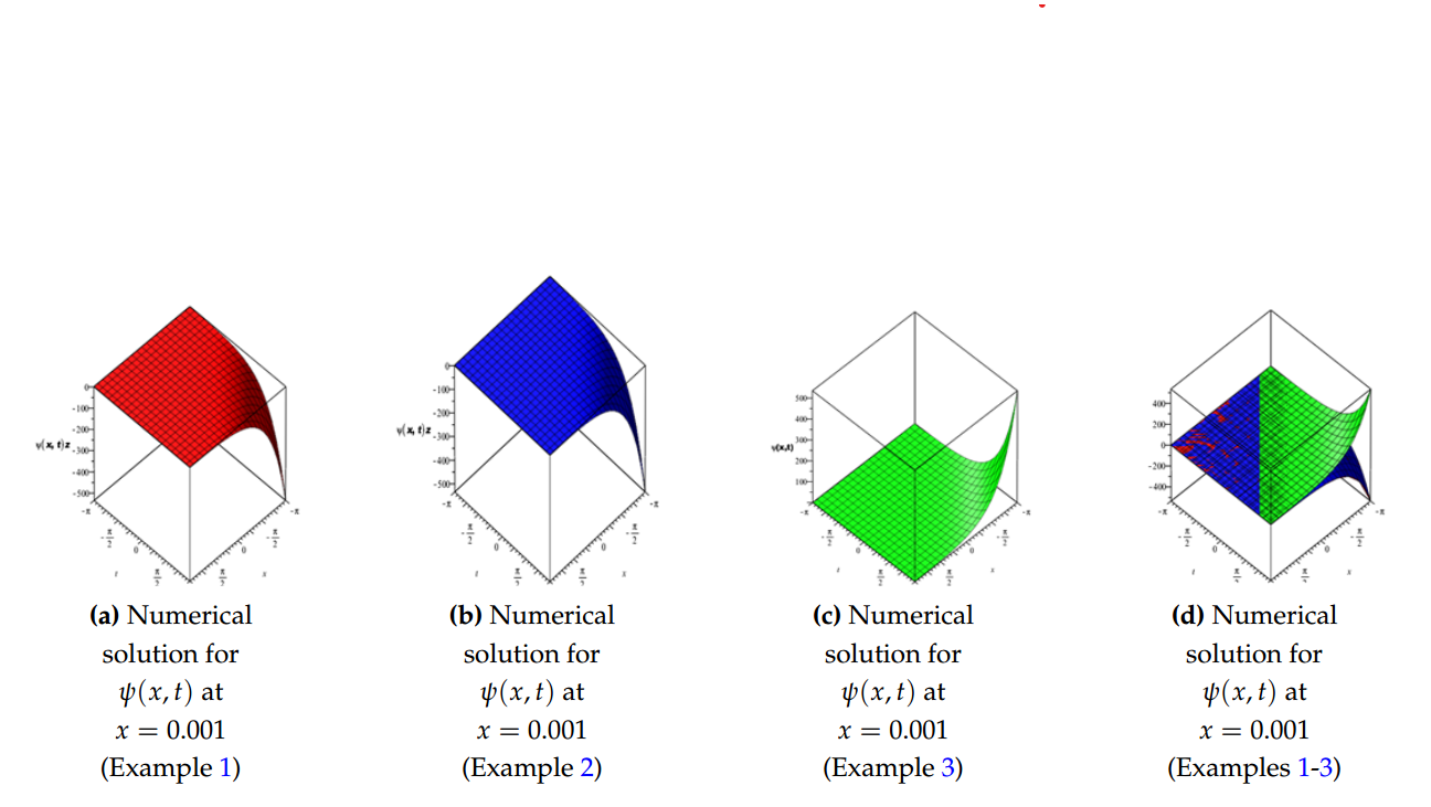
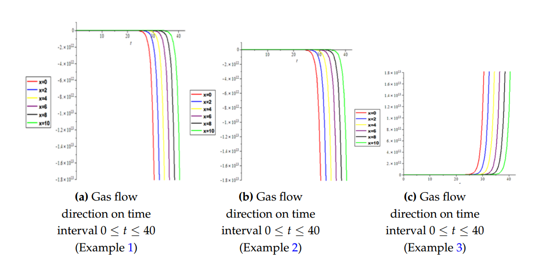
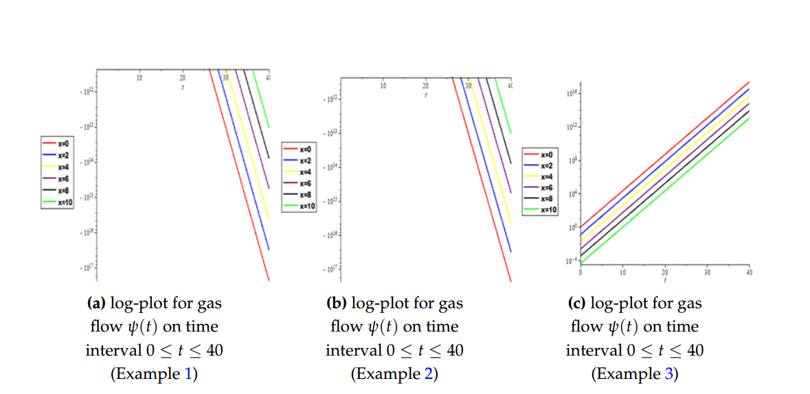
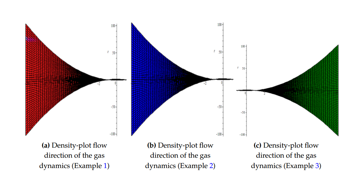
Output: See analytic-numeric solutions (15,19,23),Tables 1-3 and Figures 1(a), 1(b), 1(c), 1(d),…, Figures 4(a), 4(b), 4(c), where is the computational length and is a positive constant.
Example 1. Consider the nonlinear nonhomogeneous gas dynamic equation [2,3,4,7,10,15]
The numerical solutions for Example 1 is given in Table 1.
| \(\psi(x,t)\) | Solution | Example 1 |
|---|---|---|
| (0.001, 0.00) | Analytical | 0.00099950016662500833194464283234403 |
| MNIA | 0.00099950016662500833194464283234403 | |
| (0.001, 0.20) | Analytical | -0.2201819658998724994169694170106571 |
| MNIA | -0.2201819658998724994169694170106571 | |
| (0.001, 0.40) | Analytical | -0.4903336186074025654679095480461317 |
| MNIA | -0.4903336186074025654679095480461317 | |
| (0.001, 0.60) | Analytical | -0.8202975923459081008581182027221291 |
| MNIA | -0.8202975923459081008581182027221291 | |
| (0.001, 0.80) | Analytical | -1.2233164999636086074556190524624456 |
| MNIA | -1.2233164999636086074556190524624456 | |
| (0.001, 0.10) | Analytical | -1.7155649053185666873319827333452869 |
| MNIA | -1.7155649053185666873319827333452869 |
Example 2. Consider the nonlinear nonhomogeneous gas dynamic equation [2,3,4,7,10,15]
| \(\psi(x,t)\) | Solution | Example 2 |
|---|---|---|
| (0.001, 0.00) | Analytical | 0.00099950016662500833194464283234403 |
| MNIA | 0.00099950016662500833194464283234403 | |
| (0.001, 0.20) | Analytical | -0.2201819658998724994169694170106571 |
| MNIA | -0.2201819658998724994169694170106571 | |
| (0.001, 0.40) | Analytical | -0.4903336186074025654679095480461317 |
| MNIA | -0.4903336186074025654679095480461317 | |
| (0.001, 0.60) | Analytical | -0.8202975923459081008581182027221291 |
| MNIA | -0.8202975923459081008581182027221291 | |
| (0.001, 0.80) | Analytical | -1.2233164999636086074556190524624456 |
| MNIA | -1.2233164999636086074556190524624456 | |
| (0.001, 0.10) | Analytical | – 1.7155649053185666873319827333452869 |
| MNIA | -1.7155649053185666873319827333452869 |
Compare and apply Eq. (14) with Algorithm 1, when \(N=2\), \(\tau=1\), \(g\left(x,t\right)=-e^{t-x}\) and \(h\left(x\right)=1-e^{-x}\). We obtain approximate solution as follow:
Example 3. Consider the nonlinear homogenous gas dynamic equation [2,3,4,7,10,15]
The numerical solutions for Example 3 is given in Table 3.
| \(\psi(x,t)\) | Solution | Example 3 |
|---|---|---|
| (0.001, 0.00) | Analytical | 0.99900049983337499166805535716765597 |
| MNIA | 0.99900049983337499166805535716765597 | |
| (0.001, 0.20) | Analytical | 1.22018196589987249941696941701065712 |
| MNIA | 1.22018196589987249941696941328796801 | |
| (0.001, 0.40) | Analytical | 1.49033361860740256546790954804613177 |
| MNIA | 1.49033361860740256546741607307804137 | |
| (0.001, 0.60) | Analytical | 1.82029759234590810085811820272212919 |
| MNIA | 1.82029759234590810036634516523928928 | |
| (0.001, 0.80) | Analytical | 2.22331649996360860745561905246244569 |
| MNIA | 2.22331649996360854127633798922881128 | |
| (0.001, 0.10) | Analytical | 2.71556490531856668733198273334528698 |
| MNIA | 2.71556490531856371400530255152074189 |


In this paper, the modified new iterative algorithm (MNIA) was formulated and applied to obtain analytic-numeric solutions to the homogeneous and nonhomogeneous nonlinear gas-dynamics equation. The proposed algorithm gave analytic-numeric solutions of the three examples considered with high accuracy and good agreement with analytical solutions. The Figures 1(a), 1(b), 1(c), 1(d) depicts numerical solutions on a 3Dplot pertain to gas dynamics flow in fluid mechanics and thermodynamics, Figures 2(a), 2(b), 2(c) depict the 2D plot of gas flow in a given time interval, while 2D Logarithm-plots are presented in Figures 3(a), 3(b), 3(c) and Figures 4(a), 4(b), 4(c) demonstrated the density-plots direction of the gas flow in a gas chamber. Moreover, from the computational point of view, the proposed algorithm is faster in convergence rate, powerful and efficient in finding analytical and approximate solutions for similar nonlinear differential equations arising in applied sciences and engineering.

Algorithm 2. with(plots);
animate, animate3d, animatecurve, arrow, changecoords, complexplot, complexplot3d, conformal, conformal3d, contourplot, contourplot3d, coordplot, coordplot3d, densityplot, display, dualaxisplot, fieldplot, fieldplot3d, gradplot, gradplot3d, implicitplot, implicitplot3d, inequal, interactive, interactiveparams, intersectplot, listcontplot, listcontplot3d, listdensityplot, listplot, listplot3d, loglogplot, logplot, matrixplot, multiple, odeplot, pareto, plotcompare, pointplot, pointplot3d, polarplot, polygonplot, polygonplot3d, polyhedra\_supported, polyhedraplot, rootlocus, semilogplot, setcolors, setoptions, setoptions3d, spacecurve, sparsematrixplot, surfdata, textplot, textplot3d, tubeplot
restart; Digits:=35;
Digits:=35
N:=2;
N:=2
\(h:=1-e^{-x};\tau:=\frac{1}{2};g:=e^{t-x};\psi[0]:=h\)
\(h:=1-e^{-x}\)
\(\tau:=\frac{1}{2}\)
\(g:=e^{t-x}\)
\(\psi_{0}=1-e^{-x}\)
\(GDPDE:=value(-\tau\cdot Diff((\psi[0])^{2},x)+(\psi[0])\cdot(1-(\psi[0]))-g)\)
\(GDPDE:=-e^{t-x}\)
\(\psi[1]:=value(Int(GDPDE,t=0..t))\)
\(\psi_{1}:=e^{-x}-e^{t-x}\)
for m from 1 to N do\(\psi[m+1]:=value(Int(-\pi\cdot Diff(sum(\psi[n],n=0..m)^{2},x)+(sum(\psi[n],n=0..m))\cdot(1 -(sum(\psi[n],n=0..m)))-g,t-0..t)\)
\(-Int(-\tau\cdot Diff(sum(\psi[n],n=0..m-1)^{2},x) +(sum(\psi[n],n=0..m-1))\cdot(1-(sum(\psi[n],n=0..m-1)))-g,t=0..t))\)
end do\(\psi_2:=0\)
\(\psi_3:=0\)
\(Example[1]:=evalf(sum(\psi[k],k=0..N+1))\);
\(Example_1:=1.-1.e^{t-1.x}\)
for i from 0 by 0.2 to 1 do \(\psi[i]:=\)evalf(eval(Example[1],[x=0.001,t=i]));end do
\(\psi_0:=0.00099950016662500833194464283234403\)
\(\psi_{0.2}:=-0.2201819658998724994169694170106571\)
\(\psi_{0.4}:=-0.4903336186074025654679095480461317\)
\(\psi_{0.6}:=-0.8202975923459081008581182027221291\)
\(\psi_{0.8}:=-1.2233164999636086074556190524624456\)
\(\psi_{1.0}:=-1.7155649053185666873319827333452869\)
\(N[0]:=eval(Example[1],x=0);\)
\(N[1]:=eval(Example[1],x=2);\)
\(N[2]:=eval(Example[1],x=4);\)
\(N[3]:=eval(Example[1],x=6);\)
\(N[4]:=eval(Example[1],x=8);\)
\(N[5]:=eval(Example[1],x=10);\)
\(N_0:=1.-1.e^{t}\)
\(N_1:=1.-1.e^{t-2}\)
\(N_2:=1.-1.e^{t-4}\)
\(N_3:=1.-1.e^{t-6}\)
\(N_4:=1.-1.e^{t-8}\)
\(N_5:=1.-1.e^{t-10}\)
plot3d(Example[1],x=-Pi..Pi,t=-Pi..Pi,grid=[100,100],color=”red”)
plot([N[0],N[1],N[2],N[3],N[4],N[5]],t=0..40,color=[red,blue,yellow,purple, black,green],axes=BOXED,title=”Example 1 GDPDE”)
logplot([N[0],N[1],N[2],N[3],N[4],N[5]],t=0..40,color=[red,blue,yellow,purple, black,green],axes=BOXED,title=”Example 1 GDPDE”)
densityplot(Example1,x=0,t=-100..100,colorstyle=red;