This research presents the solution of the generalized version of Abel’s integral equation, which was computed considering the first and second kinds. First, Abel’s integral equation and its generalization were described using fractional calculus, and the properties of Orthogonal polynomials were also described. We then developed a technique of solution for the generalized Abel’s integral equation using infinite series of orthogonal polynomials and utilized the numerical method to approximate the generalized Abel’s integral equation of the first and second kind, respectively. The Riemann-Liouville fractional operator was used in these examples. Our technique was implemented in MAPLE 17 through some illustrative examples. Absolute errors were estimated. In addition, the occurred errors between using orthogonal polynomials for solving Abel’s integral equations of order \(0\ <\ \alpha \ <\ 1\) and the exact solutions show that the orthogonal polynomials used were highly effective, reliable and can be used independently in situations where the exact solution is unknown which the numerical experiments confirmed.
Keywords: Fractional calculus; Riemann-Liouville; Singular volterra integral equation; Abel’s integral; Orthogonal polynomials; Method of collocation.
1. Introduction
Fractional calculus is a branch of mathematical analysis that investigates integrals and derivatives of fractional real and complex order with their applications. Abel’s integral equation was investigated and developed by Niels Henrik Abel when he was solving and generalizing the Tautochrone problem. It enables users to compute the total time required for a particle to fall along a given curve [1]. Abel integral equations have been generalized through the theory of fractional integral equations.
Recent times, literature shows large number of engineering and scientific research involving fractional order calculus (foc), the simple reason is that it provides an accurate models of systems being considered [2]. The history [3] which is well established that several real life phenomena can not find adequate representation in the regular integer order calculus but are better described by fractional order calculus, with this, several approaches have been adopted to solve Abel’s integral equations [4, 5, 6, 7, 8, 9, 10, 11, 12, 13, 14, 15, 16, 17, 18, 19] which he generalized. Progress [20, 21] however has been made with respect to interpretation of non-integer order integral and derivative. Several numerical methods [4, 5, 7, 8, 10] for the solutions of this integral equation have been developed such as solutions in Distribution, Banach Spaces and a host of others with applications which are commonly found in modeling the dynamics of interfaces between nanoparticles and substrates [22], oscillation [23], signal processing [24], frequency dependent damping behavior of many viscoelastic materials [25], continuum and statistical mechanics [26], and economics [27].
The ideas of fractional integral operators to solve a system of generalized Abel integral equations can be found in [28], numerous attempts to solve Abel’s equations involving different types of operators can be found in the literature.
2. Materials and methods
This section, presents some definitions and mathematical preliminaries which are necessary for the evaluation of the fractional calculus [30] which will be used in this paper. The Riemann–Liouville fractional integral of order \(\alpha\) can be defined mathematically as:
where Eqs \eqref{GrindEQ__4_} and \eqref{GrindEQ__5_} are called generalized Abel’s integral equation
and weakly singular integral equations respectively.
Proposition 1.[29] For \(J^{\alpha }\), the following properties holds, \(u_{i} \in c_{\mu}\), \(i=0\dots n,\) \(\mu\ge -1\) is defined as:
witch is named after Adrien-Marie Legendre. This common differential equation can be found in physics and other branches of science. It occurs when Laplace’s equation (and related partial differential equations) are solved in spherical coordinates. Orthogonal polynomials are widely utilized in mathematics, engineering, computer science, and mathematical physics applications. Legendre polynomials are a type of orthogonal polynomial that is often used. The recurrence formula is satisfied by the Legendre polynomials \(P_n\) satisfy the recurrence formula:
where \({\delta }_{nm}\) stands for the Kronecker delta, which is \(1\) if \(m = n\) and \(0\) otherwise. On the interval \([-1,1]\), the polynomials constitute a complete set, and any piecewise smooth function can be expanded in a sequence of them.
2.2. Chebyshev polynomials
Pafnuty Chebyshev introduced Chebyshev polynomials, which was named after him are a sequence of polynomials similar to the trigonometric multi-angle formulae.
The Chebyshev differential equation is written as
The first kind of Chebyshev polynomials are a set of orthogonal polynomials defined to be the solutions to the Chebyshev differential equation and denoted by \(T_n(x).\) They are a special case of the Gegenbauer polynomial with \(\alpha =0\). They are also intimately related with trigonometric multiple-angle formulas. They are normalized such that \(T_n(1)\)=1.
Chebyshev polynomials of the first kind \(T_n(t)\) is defined to be the unique polynomials in \(x\) of degree \(n,\) defined by the relation
\(T_n(t)\ =\ cos(n\theta )\ =\ cos(n\ arccos\ t),\) where
\[t = cos\theta (0\le \theta \le \pi ),\]
is a polynomial of degree \(n(n\ =\ 0,\ 1,\ 2,\ …).\ T_n\) is called Chebyshev polynomial of degree \(n\). When \(\theta \) increases from \(0\) to \(\pi\), \(t\) decreases from \(1\) to \(-1\). Then the interval \([-1,1]\) is domain of definition of \(T_n(t)\). In addition, successive Chebyshev polynomials can be gotten by the following recursive relation
where \(w\left(x\right)={(1-x^2)}^{-\frac{1}{2}}\). The Chebyshev polynomials are orthogonal, with respect to the inner product: \(=\pi {\delta }_{ij}\).
2.3. Hermite polynomials
The Hermite polynomials, named after Charles Hermite are solutions of Hermite equation,
which is a second-order ordinary differential equation. Hermite polynomial is one of the most common set of orthogonal polynomials. The successive Hermite polynomials satisfy the recurrence relations
In the case of the Legendre, Chebyshev and Hermite polynomials, their orthogonality is with respect to possession of some standard qualities such as recurrence relation, having second-order linear differential equation and with respect to an inner product among others.
2.4. Abel’s integral equations of the first kind
Here, we consider the use of Legendre, Chebyshev and Hermite series for solving Abel’s integral equations. The derivation of the method for the first kind is given below:
Considering Eqs \eqref{GrindEQ__1_} and \eqref{GrindEQ__4_}, we have
We recommend utilizing orthogonal polynomials to approximate \(J^{1-\alpha }u\left(x\right)\) because calculating
\(J^{1-\alpha }u\left(x\right)\) is challenging, we therefore suggest using the orthogonal polynomials to approximate \(u\left(x\right)\). \(u\left(x\right)\) can be written as an infinite series of Chebyshev, Legendre and Hermite basis.
where \({\phi }_i\left(x\right)\) is the Legendre, Chebyshev or Hermite polynomials of degree \(i\).
As a result, we can get the interval \([a,\ b]\) by making a proper variable modification. With these, we can write \( u\left(x\right)\) as a truncated orthogonal series.
Using the fractional integral’s linear combination property in accordance with Proposition 1, we obtain \(J^{1-\alpha }{\phi }_i\) is all that is required. As a result, we considered
where \(b_k\), \(k=0\dots i\) are coefficients of orthogonal polynomial of degree \(i\) that are defined by \eqref{GrindEQ__7_}, \eqref{GrindEQ__10_} and \eqref{GrindEQ__14_}. Now by multiplying \eqref{GrindEQ__21_} by \(J^{1-\alpha }\), we have
Here, \(c_i\) is the result of a linear combination of \(a_i\), \(i=0,1,\dots ,\ n\). As a result, considering \eqref{GrindEQ__24_} and \eqref{GrindEQ__20_} yields the following results,
Furthermore, by replacing the roots of an orthogonal polynomial of degree \(n+1\) as collocation points in \eqref{GrindEQ__26_}, these leads to the formation of a system of linear equations, which when solved yields the needed solution of Abel’s integral equation as a truncated orthogonal series in \eqref{GrindEQ__19_}. The transformation in \eqref{GrindEQ__25_} reduces the number of times the term \(J^{1-\alpha }x^i\) is computed from \(n^2\) to \(n\).
2.5. Abel’s integral equations of the second kind
In a similar fashion, we derive for the second kind as follows:
We can rewrite \eqref{GrindEQ__5_} by considering \eqref{GrindEQ__1_} as
From \eqref{GrindEQ__26_} and \eqref{GrindEQ__28_}, after computing \(J^{1-\alpha }x^i\) and substituting the collocation points we have a system of linear equations, which when solved gives the coefficients of the approximated solution of Abel’s integral equation.
3. Results and discussion
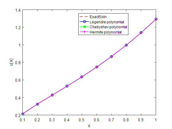
Example 1.
The Abel’s integral equation of the first kind is
\[\int^x_0{\frac{u(t)}{\sqrt{(x-t)}}dt}=e^x-1\,,\]
with exact solution \(\frac{1}{\sqrt{}\pi }e^x{\mathrm{erf} \left(\sqrt{x}\right)\ },\) where \({\mathrm{erf} \left(x\right)\ }\) is error function defined by
\[{\mathrm{erf} \left(x\right)\ }=\frac{2}{\sqrt{\pi }}\int^x_0{e^{-{\varphi }^2d\varphi }}.\]
From Eq. \eqref{GrindEQ__26_}, we have
\[f\left(x\right)=\Gamma\left(1-\alpha \right)\left(\sum^n_{i=0}{a_iJ^{1-\alpha }}{\phi }_i\left(x\right)\right)\,.\]
Here \({\phi }_i\left(x\right)\) is the Legendre, Chebyshev or Hermite polynomials of degree \(i\) as defined in \eqref{GrindEQ__18_} and \eqref{GrindEQ__19_}, we can solve for each polynomial by expressing them in terms of their recurrence relation defined earlier. With the aid of MAPLE 17 we have our numerical solution in Tables 1 and 2.
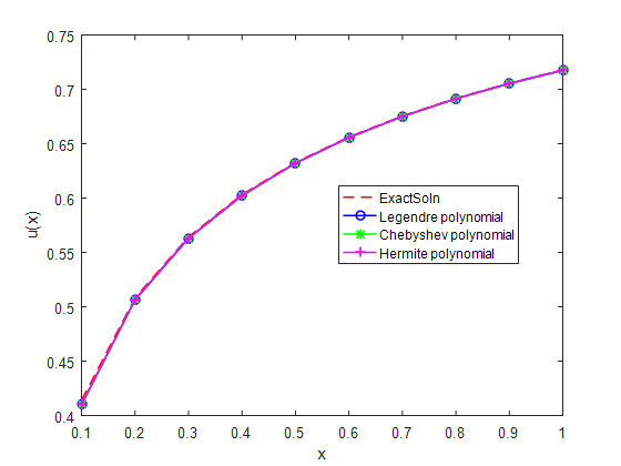
Example 2.
The Abel’s integral equation of second kind is,
\[U\left(x\right)=2\sqrt{x}-\int^x_0{\frac{u\left(t\right)}{\sqrt{\left(x-t\right)}}dt}\,.\]
The exact solution is \(1-e^{\pi x}erfc(\sqrt{\pi x})\), where \(erfc(\sqrt{\pi x})\) is a complementary error function defined as
\[erfc\left(x\right)=\frac{2}{\sqrt{\pi }}\int^{\infty }_x{e^{-{\varphi }^2d\varphi }}.\]
From Eq. \eqref{GrindEQ__28_}
\[\sum^n_{i=0}{a_i\{}{\phi }_i\left(x\right)-\Gamma\left(1-\alpha \right)\sum^n_{i=0}{J^{1-\alpha }{\phi }_i\left(x\right)}\}=f\left(x\right)\,.\]
The numerical results for this example are presented in Tables 3 and 4.
Table 1. Approximate solution, absolute errors and exact values of Example 1 for \(n=10\).
\(\boldsymbol{x}\) (step size)
Exact Value
Legendre Polynomial
Abs. Error
Chebyshev Polynomial
Abs. Error
0.1
0.2152905021
0.2139150700
0.0014
0.2139151530
0.0014
0.2
0.3258840762
0.3256471202
2.3696\(\times {10}^{-4}\)
0.3256472151
2.3686\(\times {10}^{-4}\)
0.3
0.4275656577
0.4274217109
1.4395\(\times {10}^{-4}\)
0.4274218095
1.4385\(\times {10}^{-4}\)
0.4
0.5293330732
0.5292480324
8.5041\(\times {10}^{-5}\)
0.5292481234
8.4950\(\times {10}^{-5}\)
0.5
0.6350318720
0.6349698900
6.1982\(\times {10}^{-5}\)
0.6349699660
6.1906\(\times {10}^{-5}\)
0.6
0.7470401733
0.7469949317
4.5242\(\times {10}^{-5}\)
0.7469949759
4.5197\(\times {10}^{-5}\)
0.7
0.8671875858
0.8671507681
3.6818\(\times {10}^{-5}\)
0.8671507891
3.6797\(\times {10}^{-5}\)
0.8
0.9970893764
0.997061161
2.8215\(\times {10}^{-5}\)
0.997061163
2.8213\(\times {10}^{-5}\)
0.9
1.138298578
1.138271221
2.7357\(\times {10}^{-5}\)
1.138271301
2.7277\(\times {10}^{-5}\)
1.0
1.292388093
1.29237800
1.0093\(\times {10}^{-5}\)
1.29237801
1.0083\(\times {10}^{-5}\)
Table 2. Approximate solution, absolute errors and exact values of Example 1 for \(n=10\).
\(\boldsymbol{x}\)(step size)
{Exact Value}
{Hermite Polynomial}
{Abs. Error}
0.1
0.2152905021
0.2139107224
0.0014
0.2
0.3258840762
0.3256418254
2.4225\(\times {10}^{-4}\)
0.3
0.4275656577
0.4274153293
1.5033\(\times {10}^{-4}\)
0.4
0.5293330732
0.5292405512
9.2522\(\times {10}^{-5}\)
0.5
0.6350318720
0.6349614560
7.0416\(\times {10}^{-5}\)
0.6
0.7470401733
0.7469858896
5.4284\(\times {10}^{-5}\)
0.7
0.8671875858
0.8671416940
4.5892\(\times {10}^{-5}\)
0.8
0.9970893764
0.9970529248
3.6452\(\times {10}^{-5}\)
0.9
1.138298578
1.138264975
3.3603\(\times {10}^{-5}\)
1.0
1.292388093
1.292375400
1.2693\(\times {10}^{-5}\)
Table 3. Approximate solution, absolute errors and exact values of Example 2 for \(n=10\).
\(\boldsymbol{x}\)(step size)
Exact Value
Legendre Polynomial
Abs. Error
Chebyshev Polynomial
Abs. Error
0.1
0.4140591693
0.4102961743
0.0038
0.4102960583
0.0038
0.2
0.5083515180
0.5066321249
0.0017
0.5066320640
0.0017
0.3
0.5643086686
0.5631930727
0.0011
0.5631930909
0.0011
0.4
0.6033472169
0.6025423305
8.0489\(\times {10}^{-4}\)
0.6025424464
8.0477\(\times {10}^{-4}\)
0.5
0.6328679763
0.6322458378
6.2214\(\times {10}^{-4}\)
0.6322460625
6.2191\(\times {10}^{-4}\)
0.6
0.6563234564
0.6558226175
5.0084\(\times {10}^{-4}\)
0.6558229644
5.0049\(\times {10}^{-4}\)
0.7
0.6756010623
0.6751849583
4.1610\(\times {10}^{-4}\)
0.6751854239
4.1564\(\times {10}^{-4}\)
0.8
0.6918419681
0.691489126
3.5284\(\times {10}^{-4}\)
0.6914896144
3.5235\(\times {10}^{-4}\)
0.9
0.7057865180
0.705480729
3.0579\(\times {10}^{-4}\)
0.7054813344
3.0518\(\times {10}^{-4}\)
1.0
0.7179408238
0.71767526
2.6556\(\times {10}^{-4}\)
0.7176760000
2.6482\(\times {10}^{-4}\)
Table 4. Approximate solution, absolute errors and exact values of Example 2 for \(n=10\).
\(\boldsymbol{x}\)(step size)
Exact Value
Hermite Polynomial
Abs. Error
0.1
0.4140591693
0.4103001204
0.0038
0.2
0.5083515180
0.5066359852
0.0017
0.3
0.5643086686
0.5631970712
0.0011
0.4
0.6033472169
0.6025466640
8.0055\(\times {10}^{-4}\)
0.5
0.6328679763
0.6322506550
6.1732\(\times {10}^{-4}\)
0.6
0.6563234564
0.6558280064
4.9545\(\times {10}^{-4}\)
0.7
0.6756010623
0.6751909250
4.1014\(\times {10}^{-4}\)
0.8
0.6918419681
0.6914954448
3.4652\(\times {10}^{-4}\)
0.9
0.7057865180
0.7054873805
2.9914\(\times {10}^{-4}\)
1.0
0.7179408238
0.7176818000
2.5902\(\times {10}^{-4}\)
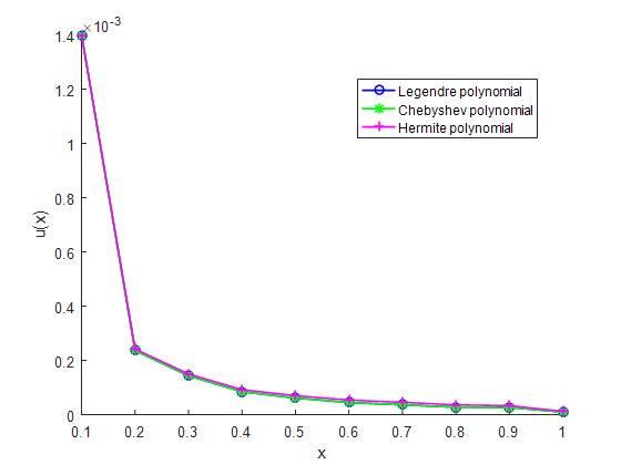
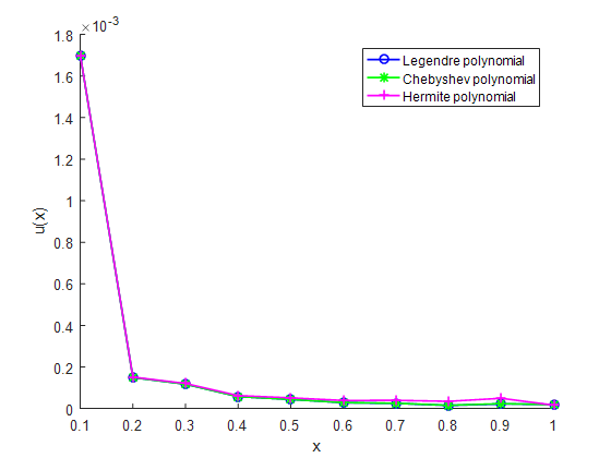
Figure 1. Numerical and exact solutions of generalized Abel’s integral equation of Example 1 with \(\alpha\) = 0.5.Figure 2. Error for generalized Abel’s integral equation for Example 1 with \(\alpha \) = \(\frac{1}{2}\).Figure 3. Numerical and exact solutions of generalized Abel’s integral equation of Example 2 with \(\alpha \) = \(\frac{1}{2}\).Figure 4. Error for generalized Abel’s integral equation for Example 2 with \(\alpha \) = \(\frac{1}{2}\).
4. Conclusion
In this research work, we implemented a method which was based on the use of infinite series of orthogonal polynomials to approximate the solution of the generalized Abel’s integral equation which was generalized with the aid of fractional calculus. Furthermore, we described the properties of Legendre, Chebyshev and Hermite polynomials. We discussed and illustrated the numerical solutions of generalized Abel’s integral equations using orthogonal polynomials. The efficiency of using orthogonal polynomials was illustrated by solving several examples of Abel’s integral equations. Orthogonal polynomials were successfully applied to solve Abel’s equations of order \(0\ < \ \alpha \ < \ 1\). All ideas were illustrated to be efficient in applying the proposed technique to several examples of that order. We found that the method is accurate and efficient in finding numerical solutions for those equations. More-over, using orthogonal polynomials demonstrate excellent approximations in comparison with the exact solutions and with other methods and solvers through the applicable domain. In addition, the occurred errors between using orthogonal polynomials for those equations of that orders and the exact solutions are small.
Acknowledgments
The authors would like to thank the referee for his/her valuable comments that resulted in the present
improved version of the article.
Conflicts of Interest:
”The author declares no conflict of interest.”
References
Podlubny, I., Magin, R. L., & Trymorush, I. (2017). Niels Henrik Abel and the birth of fractional calculus. Fractional Calculus and Applied Analysis, 20(5), 1068-1075.[Google Scholor]
Mamman, J. O., & Aboiyar, T. (2020). A numerical calculation of arbitrary integrals of functions. Advanced Journal of Graduate Research, 7(1), 11-17.[Google Scholor]
Machado, J. T., & Kiryakova, V. (2017). The chronicles of fractional calculus. Fractional Calculus and Applied Analysis, 20(2), 307-336.[Google Scholor]
Zarei, E., & Noeiaghdam, S. (2018). Solving generalized Abel’s integral equations of the first and second kinds via Taylor-collocation method. arXiv preprint arXiv:1804.08571.[Google Scholor]
Li, C., Humphries, T., & Plowman, H. (2018). Solutions to Abel’s integral equations in distributions. Axioms, 7(3), Article No. 66.[Google Scholor]
Li, C., & Srivastava, H. M. (2021). Uniqueness of solutions of the generalized Abel integral equations in Banach spaces. Fractal and Fractional, 5(3), Article No. 105.[Google Scholor]
Li, C., & Plowman, H. (2019). Solutions of the generalized Abel’s integral equations of the second kind with variable coefficients. Axioms, 8(4), Article No. 137. [Google Scholor]
Kaewnimit, K., Wannalookkhee, F., Nonlaopon, K., & Orankitjaroen, S. (2021). The solutions of some Riemann-Liouville fractional integral equations. Fractal and Fractional, 5(4), Article no. 154. [Google Scholor]
Deutsch, M., Notea, A., & Pal, D. (1990). Inversion of Abel’s integral equation and its application to NDT by X-ray radiography. NDT international, 23(1), 32-38.[Google Scholor]
Chakrabarti, A., & George, A. J. (1994). A formula for the solution of general Abel integral equation. Applied Mathematics Letters, 7(2), 87-90.[Google Scholor]
Hilfer, R., & Luchko, Y. (2019). Desiderata for fractional derivatives and integrals. Mathematics, 7(2), Article No. 149. [Google Scholor]
Garrappa, R., Kaslik, E., & Popolizio, M. (2019). Evaluation of fractional integrals and derivatives of elementary functions: Overview and tutorial. Mathematics, 7(5), Article no. 407. [Google Scholor]
Kiryakova, V. (2017, December). Use of fractional calculus to evaluate some improper integrals of special functions. In AIP Conference Proceedings (Vol. 1910, No. 1, p. 050012). AIP Publishing LLC.[Google Scholor]
Agarwal, P. (2013). Fractional integration of the product of two multivariables H-function and a general class of polynomials. In Advances in Applied Mathematics and Approximation Theory (pp. 359-374). Springer, New York, NY.[Google Scholor]
s
Kochubei, A., & Luchko, Y. (Eds.). (2019). Basic Theory. Walter de Gruyter GmbH & Co KG.[Google Scholor]
Tenreiro Machado, J. A., Kiryakova, V., Mainardi, F., & Momani, S. (2018). Fractional calculus’s adventures in Wonderland (Round table held at ICFDA 2018). Fractional Calculus and Applied Analysis, 21(5), 1151-1155.[Google Scholor]
Fawang, L., Mark M, M., Shaher, M., Nikolai N, L., Wen, C., & Om P, A. (2010). Fractional differential equations. International Journal of Differential Equations, 2010, Article ID 215856.[Google Scholor]
Ghosh, U., Sarkar, S., & Das, S. (2015). Solution of system of linear fractional differential equations with modified derivative of Jumarie type. American Journal of Mathematical Analysis, 3(3), 72-84.[Google Scholor]
Razzaghi, M. (2018). A numerical scheme for problems in fractional calculus. In ITM Web of Conferences (Vol. 20, p. 02001). EDP Sciences.[Google Scholor]
E Tarasov, V., & S Tarasova, S. (2019). Probabilistic interpretation of Kober fractional integral of non-integer order. Progress in Fractional Differentiation & Applications, 5(1), 1-5.[Google Scholor]
Podlubny, I. (2001). Geometric and physical interpretation of fractional integration and fractional differentiation. Fractional Calculus and Applied Analysis, 5(4), 367-386.[Google Scholor]
Chow, T. S. (2005). Fractional dynamics of interfaces between soft-nanoparticles and rough substrates. Physics Letters A, 342(1-2), 148-155.[Google Scholor]
Feng, Q. (2019). Oscillation for a class of fractional differential equation. Journal of Applied Mathematics and Physics, 7(7), 1429.[Google Scholor]
Panda, R., & Dash, M. (2006). Fractional generalized splines and signal processing. Signal Processing, 86(9), 2340-2350.[Google Scholor]
Bagley, R. L., & Torvik, P. J. (1983). A theoretical basis for the application of fractional calculus to viscoelasticity. Journal of Rheology, 27(3), 201-210.[Google Scholor]
Mainardi, F. (1997). Fractional calculus. In Fractals and Fractional Calculus in Continuum Mechanics (pp. 291-348). Springer, Vienna.[Google Scholor]
Baillie, R. T. (1996). Long memory processes and fractional integration in econometrics. Journal of Econometrics, 73(1), 5-59.[Google Scholor]
Gong, C., Bao, W., Tang, G., Jiang, Y., & Liu, J. (2015). Computational challenge of fractional differential equations and the potential solutions: a survey. Mathematical Problems in Engineering, 2015, Article ID 258265. [Google Scholor]
Avazzadeh, Z., Shafiee, B., & Loghmani, G. B. (2011). Fractional calculus for solving Abel’s integral equations using Chebyshev polynomials. Applied Mathematical Sciences, 5(45), 2207-2216.[Google Scholor]
Diethelm, K., Ford, N. J., & Freed, A. D. (2004). Detailed error analysis for a fractional Adams method. Numerical Algorithms, 36(1), 31-52.[Google Scholor]