Wiener polarity index of quasi-tree molecular structures

1. Introduction

Chemists in the early experiments summed up an important rule: the characteristics of compounds and its molecular structure is closely related. Inspired by this, scientists defined the indicators of molecular structure, and through the calculation of indicators they obtain the nature of the compound. Specifically, each atom in the molecular structure is represented by a vertex, and the chemical bonds between the atoms are represented by the edges, thereby converting the molecule into a graph model. The calculation of the index on the molecular structure can be transferred as the calculation of the index on the graph. The graph derived from the molecular structure is called the molecular graph. A chemical index can be thought of as a function $f:G\to {\mathbb{R}}^{+}$ that maps each molecular structure to a positive real number (See Moharir et al. [1], Udagedara et al. [2], Shafiei and Saeidifar [3], Crepnjak and Tratnik [4] for more details).

Due to the low capital requirements of such methods, there is no need to purchase experimental equipment and reagents, and so are the concerns of scientists from underdeveloped countries and regions in the Middle East, Southeast Asia. At the same time, as a branch of theoretical chemistry, its calculation results have potential applications in medical, pharmaceutical, materials and other fields, and thus are widely concerned by scholars in various fields (see Gao et al. [5], [6], [7], [8], [9], [10], [11] and [12]).
Let $G=(V(G),E(G))$ be a simple connected graph with $|V(G)|=n$. The distance $d_G(u,v)$ between vertices $u$ and $v$ in $G$ is equal to the length of the shortest path that connects $u$ and $v$. Denote $\mathcal{L}(n,d_0)$={$G$: $G$ is a quasi-tree graph of order $n$ with $G-v_0$ being a tree and $d_G(v_0)=d_0$}. The concept of quasi-tree was first introduced in Liu and Lu [13].

The Wiener polarity index is a molecular topological index introduced by Harold Wiener [14] for acyclic molecules in 1947. The Wiener polarity index of a molecular graph $G=(V,E)$ was defined as $$\begin{array}{r}{W}_p(G)=\mid \{(u,v)|d_G(u,v)=3,u,v\in V(G)\}\mid \end{array}$$

This means that Wiener polarity index of a graph $G$ is the number of unordered vertices pairs that are at distance 3 in $G$. By using its definition, Lukovits and Linert [15] demonstrated quantitative structure-property relationships in a series of acyclic and cycle-containing hydrocarbons. Besides, a physico-chemical interpretation of $W_p(G)$ was found by Hosoya [16]. Ashrafi and Ghalavand [17] determined an ordering of chemical trees with given order $n$ with respect to Wiener polarity index.

As a basic structure, tree-like structure exists in the structure of various chemical molecules such as drugs, materials and macromolecular polymers (see Heuberger and Wagner [18], Vaughan et al. [19], Bozovic et al. [20]). Therefore, the study of the tree structure helps scientists master the physicochemical properties of the structure and apply it to engineering. Although a large number of results have been obtained for the indexing of trees, the results for the quasi-tree are few, which motivates us to conduct special studies on the important indicators of the quasi-tree.

In this paper, we obtain the maximal Wiener polarity index of quasi-tree graphs of order $n$ in section 2. In section 3, we first introduce the smallest Wiener polarity index of quasi-tree graphs of order $n$, and then obtain the second smallest value.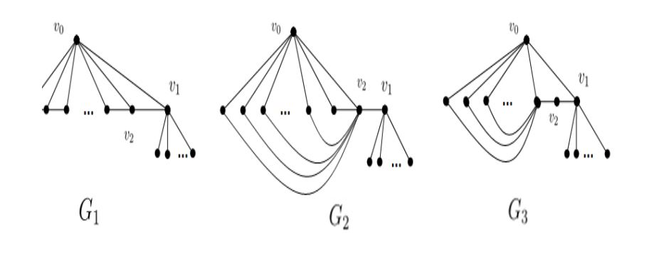

2. The maximal Wiener polarity index among all quasi-tree graphs of order $n$

First, we state some transformations on the quasi-tree with $n\ge 10,d_0\ge 3$. $\sigma$: Let $G\in \mathcal{L}(n,d_0)$ with $n\ge 10,d_0\ge 3$, $G_1$ be a condition of $G$ with $n-d_0-1$ pendant vertices adjacent to $v_1$, $G_2$ be a condition of $G$ with $n-d_0-2$ pendant vertices adjacent to $v_1$, $G_3$ be a condition of $G$ with $n-d_0-2$ pendant vertices adjacent to $v_1$. Transformation $\sigma$ on $G_i(i=1,2,3)$ is deleting a pendant vertex which is adjacent to $v_1$ and attaching a pendant vertex to $v_2$. See Fig. 1 for more details.

Lemma 2.1. $G_1$ attains the maximal value of Wiener polarity index $\lfloor \frac{n^2-7n+13}{3}\rfloor$ after applying transformation $\sigma$.

Proof. Let $G_1^{\prime }$ from $G_1$ by applying transformation $\sigma$ $m$ times on $G_2$, then there are $n-d_0-1-m$ pendant vertices adjacent to $v_1$ and $m$ pendant vertices adjacent to $v_2$. $$\begin{array}{rcl}{W}_p(G_1^{\prime })& =& m(n-d_0-1-m)+(n-d_0-1-m)(d_0-2)+m(d_0-3)\\ & =& -(m-\frac{n-d_0-2}{2}{)}^2+(\frac{n^2}{4}-3n-\frac{3}{4}{d}_0^2+2d_0+\frac{1}{2}n{d}_0+3).\end{array}$$ $W_p(G_1^{\prime })$ attains the maximal value when $m=[\frac{n-d_0-2}{2}]$, it’s equal to $m=\lfloor \frac{n-d_0-1}{2}\rfloor$. That is, when there are $\lceil \frac{n-d_0-1}{2}\rceil$ pendant vertices adjacent to $v_1$, $\lfloor \frac{n-d_0-1}{2}\rfloor$ pendant vertices adjacent to $v_2$, $W_p(G_1^{\prime })$ attains the maximal value. Let $G_1^{\ast }$ denote $G_1^{\prime }$ with the maximal value of Wiener polarity index. $$W_p(G_1^{\ast })=\lceil \frac{n-d_0-1}{2}\rceil \lfloor \frac{n-d_0-1}{2}\rfloor +\lceil \frac{n-d_0-1}{2}\rceil (d_0-3)+\lfloor \frac{n-d_0-1}{2}\rfloor (d_0-2)$$ $$=\{\begin{array}{ll}-\frac{3}{4}(d_0-\frac{n+4}{3}{)}^2+\frac{n^2-7n+13}{3},& ifn-d_{0}iseven\\ \\ -\frac{3}{4}(d_0-\frac{n+4}{3}{)}^2+\frac{4n^2-28n+49}{12},& ifn-d_{0}isdd\end{array}$$ It is easy to check that when $d_0=\lfloor \frac{n+4}{3}\rfloor$ or $\lceil \frac{n+4}{3}\rceil$, $W_p(G_1^{\ast })$ attains the maximal value $\lfloor \frac{n^2-7n+13}{3}\rfloor$.

Lemma 2.2. $G_2$ attains the maximal value of Wiener polarity index $\lfloor \frac{n^2-4n+4}{4}\rfloor$ after applying transformation $\sigma$.

Proof. Let $G_2^{\prime }$ from $G_2$ by applying transformation $\sigma$ $m$ times on $G_2$, then there are $n-d_0-2-m$ pendant vertices adjacent to $v_1$ and $m$ pendant vertices adjacent to $v_2$. $$\begin{array}{rcl}{W}_p(G^{\prime })& =& m(n-d_0-2-m)+d_0(n-d_0-2-m)\\ & =& -(m-\frac{n-2d_0-2}{2}{)}^2+\frac{n^2-4n+4}{4}.\end{array}$$ When $2d_0<n-2$, the maximal value of $W_p(G^{\prime })$ is $\lfloor \frac{n^2-4n+4}{4}\rfloor$ when $m=\lfloor \frac{n-2d_0-2}{2}\rfloor$. When $2d_0\ge n-2$, the value of $W_p(G^{\prime })$ attain the maximal value when $m=0$, it means that don't apply transformation $\sigma$ on $G_2$ and $G_2$ itself attain the maximal value, now $$\begin{array}{rcl}{W}_p(G_2)& =& d_0(n-d_0-2)\\ & =& -(d_0-\frac{n-2}{2}{)}^2+\frac{n^2-4n+4}{4}\end{array}$$ the maximal value of $W_p(G_2)$ is $\lfloor \frac{n^2-4n+4}{4}\rfloor$ when $d_0=\lceil \frac{n-2}{2}\rceil$. Combining the above conditions, let $G_2^{\ast }$ denote $G_2$ after applying transformation $\sigma$ $t(t\ge 0)$ times, the maximal value of $W_p(G_2^{\ast })$ is $\lfloor \frac{n^2-4n+4}{4}\rfloor$.

Lemma 2.3. $G_3$ attains the maximal value of Wiener polarity index $\lfloor \frac{n^2-6n+9}{3}\rfloor$ after applying transformation $\sigma$.

Proof. Let $G_3^{\prime }$ from $G_3$ by applying transformation $\sigma$ $m$ times on $G_3$, then there are $n-d_0-2-m$ pendant vertices adjacent to $v_1$ and $m$ pendant vertices adjacent to $v_2$. $$\begin{array}{rcl}{W}_p(G_3^{\prime })& =& m(n-d_0-2-m)+(n-d_0-2)(d_0-1)\\ & =& -(m-\frac{n-d_0-2}{2}{)}^2+\frac{n^2-3d_0^2+2n{d}_0-8n+12}{4}.\end{array}$$ $W_p(G_3^{\prime })$ attains the maximal value when $m=\lfloor \frac{n-d_0-2}{2}\rfloor$ or $\lceil \frac{n-d_0-2}{2}\rceil$. That is, when there are $\lceil \frac{n-d_0-2}{2}\rceil$ pendant vertices adjacent to $v_1$, $\lfloor \frac{n-d_0-2}{2}\rfloor$ pendant vertices adjacent to $v_2$, $W_p(G_3^{\prime })$ attains the maximal value. Let $G_3^{\ast }$ denote $G_3^{\prime }$ with the maximal value of Wiener polarity index. $$W_p(G_3^{\ast })=\lceil \frac{n-d_0-2}{2}\rceil \lfloor \frac{n-d_0-2}{2}\rfloor +(n-d_0-2)(d_0-1)$$ $$=\{\begin{array}{ll}-\frac{3}{4}(d_0-\frac{n}{3}{)}^2+\frac{n^2-6n+9}{3}& ifn-d_{0}iseven\\ \\ -\frac{3}{4}(d_0-\frac{n}{3}{)}^2+\frac{4n^2-24n+33}{12}& ifn-d_{0}isdd\end{array}$$ It is easy to check that when $d_0=\lfloor \frac{n}{3}\rfloor$ or $\lceil \frac{n}{3}\rceil$, $W_p(G_3^{\ast })$ attains the maximal value $\lfloor \frac{n^2-6n+9}{3}\rfloor$.

Lemma 2.4.(Hou et al. [21]) Let $U$ ba a unicyclic graph of order $n$ with $n\ge 10,g(U)\ge 4$, then $W_p(U)\le \lfloor \frac{n^2-2n-15}{4}\rfloor$.

Lemma 2.5.Let $G\in \mathcal{L}(n,2)$ with $n\ge 10$, then $$W_p(G)\le \lfloor \frac{n^2-2n-15}{4}\rfloor .$$

Proof. It is clear $G$ is a unicyclic graph. If $g(G)\ge 4$, by Lemma 2.4, $W_p(U)\le \lfloor \frac{n^2-2n-15}{4}\rfloor$. If $g(G)=3$, let $C$ denote the cycle with $V(C)=\{v_1,v_2,v_3\}$. The rest of $n-3$ vertices can only adjacent to two vertices of $V(C)$, let it be $v_2,v_3$. If all the $n-3$ vertices are only adjacent to $v_2$, $W_p(G)$ is equal to $W_P(T)$, where $T$ is a tree from $G$ by deleting the edge $v_1{v}_3$. And the maximal value of $W_p(T)$ is $\lceil \frac{n-2}{2}\rceil \lfloor \frac{n-2}{2}\rfloor$([22]). If all the $n-3$ vertices are adjacent to both $v_1$ and $v_2$, it is easy to check that the maximal value of $W_p(G)$ is $\lceil \frac{n-3}{2}\rceil \lfloor \frac{n-3}{2}\rfloor$. While $\lfloor \frac{n^2-2n-15}{4}\rfloor >\lfloor \frac{n^2-4n+4}{4}\rfloor$ when $n>10$, the Lemma is proved.

Lemma 2.6.Let $G\in \mathcal{L}(n,d_0)$ with $n\ge 10,d_0\ge 3$. Then $$W_p(G)\le W_p(G_3^{\ast }).$$ The equality holds if and only if $G\cong G_3^{\ast }$.

Proof. For the degree of $v_0$ is $d_0$, all the vertices of $G$ can be divided into two sets. The first set includes $d_0+1$ vertices for they are $v_0$ and the $d_0$ vertices are adjacent to $v_0$, denoted by $S_1$. The second set includes the rest of $n-d_0-1$ vertices, denoted by $S_2$.
Clearly, if a pair of vertices $u$ and $v$ are both in $S_1$, then $d_G(u,v)\le 2$. Suppose that $u$ and $v$ are a pair of vertices in $G$ such that $d_G(u,v)=3$, it’s either $u$ and $v$ is in $S_2$ or $u$, $v$ are in $S_1$, $S_2$, respectively.
For the pair of vertices are both in $S_2$, denote the pairs as $n_1$. For all the $n-d_0-1$ vertices can’t be in the 3 vertices of a triangle, respectively, so $n_1\le \lfloor \frac{n-d_0-1}{2}\rfloor \lceil \frac{n-d_0-1}{2}\rceil$. For the pair of vertices are in $S_1$, $S_2$, respectively. Denote the pairs as $n_2$, then $W_p(G)=n_1+n_2$. For there at least 2 vertices connect the other pair of vertices which with a distance 3, so there at least 2 vertices aren’t in the pairs with a distance 3 and at least one is from $S_1$. The less vertices aren’t in, the more of the value $n_1+n_2$. The maximal value of $n_2$ will be $d_0(n-d_0-2)$ if just one is from $S_1$, and then the other one is from $S_2$, so the possible maximal value of $n_1$ is $\lfloor \frac{n-d_0-2}{2}\rfloor \lceil \frac{n-d_0-2}{2}\rceil$. The maximal value of $n_2$ will be $(d_0-1)(n-d_0-2)$ if there are two from $S_1$ and one is from $S_2$, so the possible maximal value of $n_1$ is $\lfloor \frac{n-d_0-2}{2}\rfloor \lceil \frac{n-d_0-2}{2}\rceil$. The maximal value of $n_2$ will be $(d_0-2)(n-d_0-1)$ if there are three from $S_1$ and none is from $S_2$, so the possible maximal value of $n_1$ is $\lfloor \frac{n-d_0-1}{2}\rfloor \lceil \frac{n-d_0-1}{2}\rceil$. $G_1$, $G_2$, $G_3$ attain the three maximum values of $n_2$ for $(d_0-2)(n-d_0-1),d_0(n-d_0-2),(d_0-1)(n-d_0-2)$. Using the same notations in transformation $\sigma$.
$\bullet$ Case 1: $n_2$ attains one of the maximal value $(d_0-2)(n-d_0-1)$ in $G_1$. After applying transformation $\sigma$, $n_1$ attains the maximal value $\lfloor \frac{n-d_0-1}{2}\rfloor \lceil \frac{n-d_0-1}{2}\rceil$ in $G_1^{\ast }$, but $n_2$ decreased to $\lceil \frac{n-d_0-1}{2}\rceil (d_0-2)+\lfloor \frac{n-d_0-1}{2}\rfloor (d_0-3)$, it’s between $(d_0-3)(n-d_0-1)$ and $(d_0-2)(n-d_0-1)$. $n_1+n_2$ will attain the maximal value of $\lfloor \frac{n^2-7n+13}{3}\rfloor$ in $G_1^{\ast }$.
$\bullet$ Case 2: $n_2$ attains one of the maximal value $d_0(n-d_0-2)$ in $G_2$ while the value of $n_1$ is 0. After applying transformation $\sigma$, $n_1$ attains the possible maximal value $\lfloor \frac{n-d_0-2}{2}\rfloor \lceil \frac{n-d_0-2}{2}\rceil$, but $n_2$ decreased. $n_1+n_2$ will attain the maximal value of $\lfloor \frac{n^2-4n+4}{4}\rfloor$ in $G_2^{\ast }$.
$\bullet$ Case 3: $n_2$ attains one of the maximal value $(d_0-1)(n-d_0-2)$ in $G_3$, it’s smaller than that in $G_2$, but after applying transformation $\sigma$, $n_1$ attains the possible maximal value $\lfloor \frac{n-d_0-2}{2}\rfloor \lceil \frac{n-d_0-2}{2}\rceil$ while the value of $n_2$ unchanged. $n_1+n_2$ will attain the maximal value of $\lfloor \frac{n^2-6n+9}{3}\rfloor$ in $G_3^{\ast }$.
From case 1 and case 2, the conclusion is that $n_1$ and $n_2$ can’t attain the maximal value simultaneously in $G_1^{\ast }$ and $G_2^{\ast }$. It’s only in $G_3^{\ast }$ that $n_1$ and $n_2$ attain the maximal value simultaneously. So we just need to compare the maximal value of $n_1+n_2$ in $G_1^{\ast }$, $G_2^{\ast }$, $G_3^{\ast }$. By Lemma 2.1, 2.2, 2.3, $W_p(G_3^{\ast })$ attains the maximal value.

By combining all the conclusions above, we yield our first main result in this paper which is stated below.

Lemma 2.7.Let $G\in \mathcal{L}(n,d_0)$ with $n\ge 4,d_0\ge 2$.

• (1) If $n=4$, then $W_p(G)\le 1$.
• (2) If $n=5$, then $W_p(G)\le 2$.
• (3) If $n=6$, then $W_p(G)\le 3$.
• (4) If $n=7$, then $W_p(G)\le 7$.
• (5) If $n=8$, then $W_p(G)\le 9$.
• (6) If $n=9$, then $W_p(G)\le 12$.
• (7) If $n\ge 10$, then $W_p(G)\le \lfloor \frac{n^2-6n+9}{3}\rfloor$.

3. The smallest and second smallest Wiener polarity index among all quasi-tree graphs of order $n$

Let $G\in \mathcal{L}(n,d_0)$. Then $W_p(G)\ge 0$. In the graph $G_4$, no matter what the value of $d_0$ is, all vertices are adjacent to $v_1$, then there isn’t any pair of vertices whose distance is greater or equal to 3. So the smallest Wiener polarity index among all quasi-tree graphs of order $n$ is 0. The graph that attains the smallest Wiener polarity index is not unique, $G_5$ is just an example.

Lemma 3.1. (Liu and Liu [22]) Let $G$ be an unicyclic graph of order $n$, and $W_p(G)>0$. Then $W_p(G)\ge n-4$.

By Lemma 3.1, if $G\in \mathcal{L}(n,2)$, the second smallest Wiener polarity index of $G$ is $n-4$. As for $G\in \mathcal{L}(n,d_0)$ with $d_0\ge 3$, all the vertices of $G$ can be divided into two sets. The first set includes $d_0+1$ vertices for they are $v_0$ and the $d_0$ vertices are adjacent to $v_0$, denote the set by $S_1$ and the $d_0+1$ vertices by $v_0$, $v_{0_1}$, $v_{0_2},\cdots ,v_{0_{d_0}}$. The second set includes the rest of $n-d_0-1$ vertices, denote the set by $S_2$ and the $n-d_0-1$ vertices by $v_1$, $v_2$, … $v_{n-d_0-1}$.

Lemma 3.2. Let $G\in \mathcal{L}(n,d_0)$ with $d_0\ge 3$. Let $v_1,v_2\in S_2$, and $d_G(v_1,v_2)\ge 3$. Then the two conditions can’t hold simultaneously, for they are the distance between $v_1$ and every vertex of $S_1$ is less than or equal to 2, the distance between $v_2$ and every vertex of $S_1$ is less than or equal to 2.

Proof. For $d_G(v_1,v_2)\ge 3$, without loss of generality, let $d_G(v_1,v_2)=3$ and the path of length 3 is $v_1{v}_i{v}_j{v}_2$. For $d_0\ge 3$, there at least exists one vertex $v_{0_1}$ in $S_1$, while $v_{0_1}$ is different from $v_i$ and $v_j$(even if $v_i$, $v_j$ are both in $S_1$ ), the distance between $v_{0_1}$ and $v_1$ is less than or equal to 2, so $v_{0_1}$ is adjacent to $v_1$ or the vertices which are adjacent to $v_1$(let it be $v_i$) and the distance between $v_{0_1}$ and $v_2$ is greater or equal to 3.

Lemma 3.3. Let $G\in \mathcal{L}(n,d_0)$ with $d_0\ge 3$. If $W_p(G)>0$, there at least exist a vertex $v_i$ in $S_2$ such that $d_G(v_i,v_j)\ge 3$, while $v_j\in S_1$.

Proof. If the distance between any a vertex in $S_1$ and every vertex in $S_2$ is less than or equal to 2. In terms of the condition of Lemma 3.2, there isn’t any pair of vertices with a distance of 3 in $S_2$. And it’s clear that there isn’t any pair of vertices with a distance of 3 in $S_1$, so $W_p(G)=0$.

Lemma 3.4. Let $G\in \mathcal{L}(n,d_0)$ with $d_0\ge 3$. If there are $t(t\ge 2)$ vertices in $S_2$ satisfying the condition that the distance between each vertex and every vertex in $S_1$ is less than or equal to 2, the $t$ vertices can only be composed by two forms:
Case 1. If $t=2$, the 2 vertices must be adjacent.
Case 2. If $t\ge 2$, the $t$ vertices must be adjacent to one common vertex, where the common vertex is $v_{0_i}$ in $S_1$.

Proof. By means of Lemma 3.3, the distance between any two of the $t$ vertices is less than or equal to 2. If $t=2$, the two vertices are either adjacent or adjacent to one common vertex, where the common vertex is $v_{0_i}$ in $S_1$. When the two vertices are adjacent, every $v_{0_i}$ in $S_1$ should be adjacent to one and only one of them. When the two vertices are adjacent to one common vertex(let it be $v_{0_1}$), the other $v_{0_i}$ in $S_1$ should be adjacent to $v_{0_1}$.
If $t=3$ and the 3 vertices compose a path of length 2, denote the path by $v_1{v}_2{v}_3$. For the distance between $v_0$ and $v_t$ is 2, $v_1$, $v_2$ and $v_3$ must be adjacent to 3 different $v_{0_i}$ in $S_1$. Let $v_{0_1}$ be the vertex that $v_1$ adjacent to, then the distance between $v_{0_1}$ and $v_3$ is 3. So the 3 vertices can only adjacent to one common vertex, where the common vertex is $v_{0_i}$ in $S_1$. Similarly, if $t>3$, the $t$ vertices must be adjacent to one common vertex, where the common vertex is $v_{0_i}$ in $S_1$.

Now, we prove our second main result.

Theorem 3.5. Let $G\in \mathcal{L}(n,d_0)$. If $W_p(G)>0$ and $d_0\le n-3$ then $$W_p(G)\ge n-d_0-2.$$

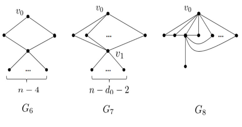
Proof. (1)If $d_0=2$, by Lemma 3.1, $W_p(G)\ge n-d_0-2=n-4$. $G_6$ is an example that attains the smallest value.
(2)If $3\le d_0\le n-3$, let $v_1$, $v_2$, … , $v_i$ in $S_2$ satisfy the condition that the distance between any one of them and every vertex in $S_1$ is less than or equal to 2. By Lemma 3.3, $i<n-d_0-1$, let $v_{i+1}$, … $v_{n-d_0-1}$ be the rest vertices satisfy the condition that the distance between any one of them and every vertex in $S_1$ is greater or equal to 3.

$\bullet$ Case 1. If $i=1$, for everyone of the rest $n-d_0-2$ vertices in $S_2$, there exist at least one vertex in $S_1$ such that the distance between the two vertices is greater or equal to 3, then $W_p(G)\ge n-d_0-2$.
$\bullet$ Case 2. If $i=2$, and $v_1$, $v_2$ satisfy the case 1 in Lemma 3.4.
Subcase 1. $v_3$ is adjacent to $v_1$ or $v_2$, let it be $v_1$. Then $d_G(v_3{v}_0)=3$, $d_G(v_3{v}_{0_2})=3$, where $v_{0_2}$ is in $S_1$ and $v_2$ is adjacent to it.
Subcase 2. $v_3$ is adjacent to $v_{0_1}$, $v_{0_1}$ must be adjacent to $v_1$ or $v_2$, let it be $v_1$. Then $d_G(v_3{v}_{0_2})=3$, if $v_{0_2}$ is adjacent to $v_1$. $d_G(v_3{v}_{0_2})=3$, if only $v_{0_1}$ in $S_1$ is adjacent to $v_1$ and the path is $v_3{v}_{0_1}{v}_0{v}_{0_2}$, where $v_{0_2}$ is adjacent to $v_2$.
Anyway, there are at least 2 pairs vertices with a distance of 3 for $v_3$. As for $v_4$,…, $v_{n-d_0-1}$, similar to the analysis of $v_3$, there are more than $n-d_0-4$ pairs of vertices with a distance of 3 for them. So there are more than $n-d_0-2$ pairs of vertices for $v_i(i=1,2,\dots ,n-d_0-1)$.
$\bullet$ Case 3. If $i\ge 2$, and $v_1$, $v_2$, … , $v_i$ satisfy the case 2 in Lemma 3.4, that is $v_1$, $v_2$, … , $v_i$ are adjacent to one common vertex(let it be $v_{0_1}$).
Subcase 1. $v_{i+1}$ is adjacent to one of $v_1$, $v_2$, …, $v_i$(let it be $v_1$), then $d_G(v_{i+1}{v}_2)$, $d_G(v_{i+1}{v}_3)$,…, $d_G(v_{i+1}{v}_i)$ are all 3, and $d_G(v_{i+1}{v}_0)=3$.
Subcase 2. $v_{i+1}$ is adjacent to one $v_{0_i}$, where the $v_{0_i}$ should be different from $v_{0_1}$(let it be $v_{0_2}$). Then $d_G(v_{i+1}{v}_1)$, $d_G(v_{i+1}{v}_2)$,…, $d_G(v_{i+1}{v}_i)$ are all 3.
Anyway, there are at least $i$ pairs of vertices with a distance of 3 for $v_{i+1}$. As for $v_{i+2}$,…, $v_{n-d_0-1}$, similar to the analysis of $v_{i+1}$, there are more than $n-d_0-2-i$ pairs of vertices with a distance of 3 for them. So there are more than $n-d_0-2$ pairs of vertices for $v_i(i=1,2,\dots ,n-d_0-1)$.
In general, $W_p(G)\ge n-d_0-2$ if $i\ge 2$, $W_P(G)>n-d_0-2$ if $i=1$. That is, when there is only one vertex $v_1$ satisfying the condition that the distance between $v_1$ and every vertex in $S_1$ is less than or equal to 2, $W_p(G)$ can attain the smallest value $n-d_0-2$.

Let $G\in \mathcal{L}(n,d_0)$. The second smallest value of $W_p(G)$ is $n-d_0-2$ if $d_0\le n-3$(see $G_7$). The second smallest value of $W_p(G)$ is 1 if $d_0=n-2$(see $G_8$).

Conclusion

In this paper, we mainly study the Wiener polarity index of quasi-tree molecular structures, and the maximal value and the second smallest value of quasi-tree graphs with fixed order are presented. Since Wiener polarity index has been widely applied in the analysis of both the melting point and boiling point of chemical compounds and QSPR/QSAR study, and quasi-tree structure is commonly appeared in the molecular structures, the results obtained in this paper have promising prospects of application in the field of chemical, medical and pharmacy engineering.

Competing Interests

The authors declare no competing interest.