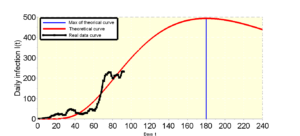
A state of health emergency has been decreed by the Togolese government since April 01 for a period of 3 months, with the introduction of a curfew which ended on June 9, following the first case of contamination of the corona Sars- Cov-2 in Togo, case registered on March 06, 2020. This first wave of contamination started from March 19. The data observed in Togo are cases tested positive and which are cured using a protocol based on the combination of hydroxychloroquine and azithromycin. This manuscript offers a forecast on the number of daily infections and its peak (or maximum), then the cumulative numbers of those infected with the covid’19 pandemic. The forecasts are based on evolution models which are well known in the literature, which consist in evaluating the evolution of the cumulative numbers of infected and a Gaussian model representing an estimate of the number of daily infections for this first wave of contamination. over a period of 8 months from the sample of observed data.
Nowadays, the economic and political societal world is very interested in understanding the temporal evolution of the total number of infections of the population by the current Sars-Cov-2 virus (corona). The most significant problems are the total duration and peak hour of the course of the infection, as well as the maximum number of daily or cumulative infections (see [1,2]). It would be very useful for many people to have an estimate of the evolution over time of this pandemic. The purpose of this manuscript is to provide such an estimate based on two simplified models for the temporal evolution of those infected with the pandemic COVID’19 in Togo. This is to allow decision-makers to take appropriate measures to control and reverse the infection curve in the short and medium term.
A sentence from Box and Draper [3], taken up by Cheng in his article aimed at explaining how to build a model good enough (Cheng et al. [4]), sums up the situation fairly well: basically, all the models are wrong, but some are useful (\(\cdots\)). This is reassuring! It should indeed be borne in mind that in no case will the model be able to accurately reflect reality. The aim of modeling is to find an expression of the model that comes closest to reality (that is to say with the best possible adequacy to the data), while remaining interpretable in a simple way, this last point being fundamental. The parameters of the model must refer to a visual characteristic of the curve corresponding to the model so that their interpretation is easy. So a model good enough may be fine. An example given by Cheng [4] is the following: one can imagine that the exact model in the studied population could be nonlinear, while the modeling based on the available data of a sample of this population could only be done linearly. Such a linear model could still be good enough to approach the exact model. The exact model for the entire population may be more complex than necessary to describe the sampled subpopulation. Among the models theoretically usable on these sample data, there is necessarily one which is the best (Cheng et al., [4]). However, there are undoubtedly several models which are close enough to be considered as good enough to meet the objectives of the analysis. We use in our paper two complex models, i.e., non-linear models available in the literature. The list of types of nonlinear models is non-exhaustive, as is that of their equations, which can take various forms (Campana and Jones, [5]). Despite their complexity, these models do not explicitly incorporate the effect of the drug. In fact, all these models describe an evolution or growth, but only through a function which is not linked to the treatment, to the dose administered, or to the administration protocol followed. Thus it is not possible to use these models to simulate changes in therapeutic strategies. They are nevertheless very sufficient to calculate metrics predictive of the evolution of a pandemic. In our study, we are interested, given the data we have, on the Bernouilli and Gompertz models for the cumulative numbers of infections and then on the Gaussian model for daily infections allowing us to have the peak to predict.
As non-virologists, we do not know the recent literature on virology. Nevertheless, we, the team of mathematicians, hope that in these difficult times, an estimate by impartial non-experts can be welcomed by virology specialists as well as by the general population. We base our parameter estimates on information accessible to the public from the Togolese government site and these data are collected from March 19, 12 days after the first case of contamination. The determination of the estimators of the parameters of each of the models is first obtained mathematically using the log-likelihood method and then numerically using the SCILAB software since these estimators are complicated or even impossible to obtain explicitly.
The interest of these descriptive models lies in the fact that they can be written implicitly, thus allowing rapid implementation and calculations. The impact of each parameter can also be studied.
Numerical simulations and empirical epidemic data on the WHO site indicate that the temporal evolution of epidemic waves is characterized by a slow exponential increase at the beginning and then early after a given time, until a maximum pronounced is reached. As explained above, we adopt a Bernouill model and a Gompertz model for the time course of cumulative infections and a Gaussian model for daily infection and then explore its consequences. We denote by \(N(t)\) (or simply \(N\)) the cumulative number of infections per day.
We suppose that the infection rate \(\nu\) is of the form \(\nu(N)=\nu_0-\nu_1N^{\theta}\) and that the effect or the rate of the barrier measures which slow down the speed \(\mu\) is of the form \(\mu(N)=\mu_0+\mu_1N^{\theta}\) where \(\nu_0,\nu_1,\mu_0, \mu_1,\; \text{and}\; \theta\) are positive constants such as \(\nu_0-\mu0>0 \) and \(\theta>0\). In other words, the infection rate decreases with the cumulative number of infected people in the population while the effect of barrier measures increases. So we have \begin{equation*} \displaystyle\frac{d N}{dt}=\nu(N)I – \mu(N)N = (\nu_0 – \mu_0)N – (\nu_1 + \mu_1)N^{\theta+1}. \end{equation*} If we set \(\nu_i=\displaystyle\frac{n_i}{\theta}\) and \(\mu_i=\displaystyle\frac{m_i}{\theta}\) où \(i\in \{0,1\}\), then we have
The formula (1) is then the deterministic model of Bernouilli.
Gompertz establishes a growth model which will later be one of the most used in biology and medicine. Particularly realistic and in line with the observations in vivo carried out, the Gompertz model describes, first a slow growth followed by an exponential acceleration before finally stabilizing and reaching its maximum size while the model of Benouilli is different from that of Gompertz by two aspects: growth accelerates very slowly and the slowdown is brutal.
The Gompertz model is described by the equation
Remark 1. When \(\theta = 1\), le modèle (1) is reduced to the logistic or Verhulst model. When \(\theta \longrightarrow 0^+\), the Bernouilli model (1) becomes an approximation of the Gompertz model (2). Indeed, \[\displaystyle\lim_{\theta \longrightarrow 0^+}\displaystyle\frac{r}{\theta}\left[ 1 – \left(\displaystyle\frac{N(t)}{K}\right)^\theta\right]=-r\log\left(\displaystyle\frac{N(t)}{K}\right).\]
Proposition 1. The solution of nonlinear ODE (1) is given by the formula
In particular for \(\theta=1\) (Verhulst model), we have
Proof. Just change the variable \(\omega(t)=\log\left(\displaystyle\frac{N(t)}{K} \right)\) then after an integration, we get the solution (3).
Proposition 2. The solution of nonlinear ODE (2) is expressed by the formula
Proof. Proposition 2 is a corollary of Proposition 1 (from Remark 1). By a simple limit calculation when \(\theta\longrightarrow 0^+\) of (3), we get the solution (5).
Remark 2. Note that in both cases we have
All the parameters of the two aforementioned models are unknown. The objective of the following paragraph is to provide estimators of all these parameters from a sample of size \(n=80\) using an optimization method based on the log-likelihood then their numerical values (thanks to an algorithm implemented in the SCILAB software in the absence of their explicit values) which are very complex or even impossible to determine. Then we do simulations over 240 days (8 months from March 06) for each of the two models from the estimators obtained, to have forecasts on the cumulative number \(\overline{N}\) of infected on the 240th day (which falls on the end of October). Finally, the algorithm implemented in the software gives us the sum of the squares of the differences (RSS) between the observed data and the estimated data. This quantity of RSS also allowed us to choose the best model.
Consider the \(n\) measurement points \((t_i,y_i)_{\{1\leqslant i \leqslant n\}}\) where \(t_i\) represents the day \(i\) from the date of the first case of contamination and \(y_i\) the cumulative number of infected on date \(t_i\). It is assumed that each measurement has a measurement error which is i.i.d., distributed according to a normal law of zero mean and standard deviation \(\sigma\). The model predicts a functional relationship between the variable \(t\) and \(y\), depending on a set\(\beta\) of parameters, where \(\beta=(r,K,\theta)\) for the Equation (1) and \(\beta=(r,K)\) for the Equation (2) such that \(y(t)=N(t,\beta)\). What we observe is therefore \(y(t)=N(t,\beta)+\varepsilon\) where \(\varepsilon\) is a random variable following a normal law of zero mean and unknown variance \(\sigma\). The probability density of \(\varepsilon\) is that of \(\mathcal{N}(0,\sigma^2)\). Consequently each observation is the realization of a random variable \(Y \leadsto \mathcal{N} (N(t,\beta), \sigma^2)\).
The likelihood function for a sample of \(n\) observations is, except for a positive constant factor:


Modeling growth often involves comparing several models of different equations on the same dataset. This comparison allows the choice of the model that best fits the data. In general, we use the Akaike Information Criterion (AIC), a measure of the quality of a model, widely used for forecasting purposes and especially for small data. It is written in the following form
The fact that we are in the framework of deterministic models and that errors are assumed i.i.d. normally distributed \(\mathcal{N}(0,\sigma^2)\) then (9) is written in the form
| RSS | 23901.245 | 23909.088 |
|---|---|---|
| \(\hat{\sigma}^2\) | 298.765 | 298.864 |
| \(\hat{\sigma} \) | 17.285 | 17.288 |
| AIC | 15.400 | 17.400 |
| AIC\(_c\) | 15.555 | 17.716 |
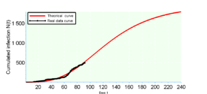
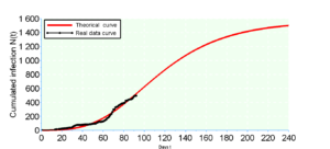
According to the calculations we see that the Gompertz model ensures a better fit because its \(AIC_c\). This result is predictable because the rate of increase \(r\) is average equal to \(2\%\) for the real data whereas the rate of increase of the Bernoulli model is \(r=2.3\%\) against \(r=1.9\%\) from Gompertz. It should be remembered that the 240th day falls on the end of October from March 6 which is the first day, so we make a prediction of \(\overline{N}_G=1784\) for the Gompertz model against \(\overline{N}_B=1508\) for the Bernouilli model with a standard deviation \(\hat{\sigma}=17.28\) (which constitutes the margin of error) for the two models.
In this particular case, the AIC gives the best fit, which is not the case in general. Other equivalent definitions of AIC may be used. In this study we chose to minimize this criterion. We can choose to maximize it. These criteria are close to an affine transformation (that is to say a near multiplicative coefficient and a translation by a constant). Numerical values may be different, but the best criteria will be the same.
This Gaussian model is widely used in the analysis of lifetimes (see Agbokou et al., [8,9]).

The purpose of this study is to alert the Togolese state to a probable early development of the pandemic despite this deceptive stability which is only a temporary slowdown over a short period. The investigations carried out in this manuscript take into account the resumption of activities after the Togolese state’s suspension of the curfew, such as the reopening of classes and places of worship, etc. If the barrier measures are not put in place for the resumption of classes in schools, universities and places of worship, we can witness a sudden explosion of figures. The Togolese government has made it compulsory to wear a muffler, which is beneficial and will reduce the speed of contamination if the Togolese state makes the masks available to the population, otherwise there will be a spike in the figures . Note that the daily samples for covid19 screening tests in Togo provide an average rate of \(2.2\%\) of cases detected with or without asymptomatic covid19 and the fatality rate is on average around \(2.5\%\). It should also be noted that among the \(2.5\%\) of deaths observed, more than \(50\%\) suffered from certain pathologies which are often poorly treated for lack of means. In addition, in some places of detention, all the detainees were taken, which reassures a little compared to the risk of contacts. The current health situation has provoked the fear of seeking treatment for other pathologies in hospitals, especially those which are requisitioned for the treatment of covid’19. As a consequence of this situation of fear or fear, many diseases have taken their toll. For example, in 5 months 2020 the country recorded more than 320 deaths linked to malaria against 13 linked to covid19, which is alarming. The state made a lot of effort in the case of covid’19 even if it is not what we hope. However half of this energy must be deployed to save the population from the rage of malaria as well as other diseases such as HIV-AIDS and tuberculosis which are being left in the background.
A mathematical model capable of analyzing the interaction between the corona virus, the patient’s host cells and the protocol administered to patients, will be the subject of our future research after a reasonable period of healing of the patient.