When mathematical models of biological phenomena deal with an unknown parameter, it is often assumed that such a parameter follows a normal distribution. This introduces a symmetry assumption into the model. The purpose of this paper is to investigate and quantify the effect of asymmetry on model prediction. We introduce an asymmetry into a model of sexual conflict and toxin allocation by replacing a normal distribution by a shifted beta distribution. This way, we can naturally consider a large family of continuously changing distributions. We isolate the effect of skewness on the model prediction and demonstrate that in most cases, increasing skewness causes a slight increase in optimal toxicity allocation. We conclude that overall, the effect of the skewness is much smaller than the effect of the mean. In fact, for the particular model we studied, skewness does not seem to affect qualitative predictions.
Symmetry is present everywhere in the biological world as well as in mathematical models that describe such a word [1]. The models include many parameters, most of which are known only up to a certain degree of certainty. Many approaches have been adopted to understand and study the uncertainty in parameter values; see, for example, [2]. The approaches typically assume that a model parameter follows a certain distribution symmetric around its mean, such as uniform or normal distribution.
Similarly, when mathematical models in biology assume that a quantity follows a distribution, such a distribution is typically normal, i.e., symmetrical. This was also the case of [3] that investigated the evolution of male seminal toxicity. Their model described below in Section 2.1 considers a female benefit of remating as one of its parameters. This parameter was considered to be a random variable following a normal distribution with a given mean and variance.
The purpose of the paper is to determine the effect of symmetry on the model prediction. We adopt the core of the model used by [3] but we model the female benefits using the shifted beta distribution. This allows us to naturally consider a large family of continuously changing distributions with a fixed mean and variance and varying skewness. We replicate the analysis done in [3] for this modified model, allowing us to isolate the effects of the asymmetry on the model outcomes.
We adopt a model of seminal toxins allocation developed in [3]. For simplicity, we assume that females can mate once or twice. Multiple mating is typically associated with net benefits [4,5] which we will denote by \(f\). The benefits may vary from female to female, based on many factors. [3] assumed that \(f\) is normally distributed, i.e., \(f\) follows a distribution that is symmetric about its mean. To properly assess the effect of the (a)symmetry, we consider \(f\) to follow a shifted \(Beta(\alpha,\beta)\) distribution for appropriate parameters \(\alpha\) and \(\beta\); we will discuss the details of the distribution in Section 2.2 .
Males may transfer toxins to a female during mating. A female that acquires a total \(t\) toxins from all mates suffers a cost \(c(t)\). It is assumed that \(c(0) = 0\), \(c'(t)>0\) and \(c''(t)>0\), i.e., there is no cost if males do not transfer any toxins and the cost increases at an accelerating rate. As in [3], we considered cost functions in the form \(c(t) = t^3\).
We are interested in the optimal amount of toxins male should transfer to a female during the mating. More formally, we are interested in the evolutionary stable strategy, i.e., a strategy that, if adopted by everybody in the population, cannot be invaded by a rare mutant strategy. By [6], it means that we are looking for \(t_{NE}\) such that \[\label{eq:tNE} w(t_{NE}, t_{NE}) > w(t,t_{NE}), t\neq t_{NE}, \tag{1}\] where \(w(t,\hat{t})\) is a benefit to a male using \(t\) when everyone else in the population uses \(\hat{t}\).
To evaluate \(w(t,\hat{t})\), we need to account for all three of the following scenarios.
The focal male mates with a previously unmated female and the female does not benefit from second mating. This happens if \(1+f-c(t+\hat{t})< 1-c(t)\), i.e. the benefit of a single mating normalized to \(1\), plus the additional benefit of remating, \(f\), minus the total costs of mating with males transferring \(t\) and \(\hat{t}\) toxins, \(c(t+\hat{t})\), is less than the single mating benefit \(1\) minus the current cost of mating, \(c(t)\). If this is the case, the focal male gets 100% of the offspring, i.e., female’s fitness which is \(1-c(t)\).
The focal male mates with a previously unmated female and the female benefits from second mating (and thus mates with another male). This happens if \(f>c(t+\hat{t}) -c(t)\). If \(m\) is expected paternity share of the second male to mate, the focal male gets a fraction \((1-m)\) of the total female’s fitness which is \(1+f-c(\hat{t}+t)\).
The focal male mates with a previously mated female who continued to mate the second time because her expected benefits from the second mating outweighed the costs. This happens if \(f>c(2\hat{t}) – c(\hat{t})\). In this case, the male gets a fraction \(m\in(0,1)\) of the female’s fitness which is \(1+f-c(\hat{t}+t)\).
Thus, \[\label{eq:W} \begin{split} w(t,\hat{t}) = \int_{-\infty}^{c(t+\hat{t}) -c(t)} \big[1-c(t)\big] p(f)df + \int_{c(2\hat{t}) -c(\hat{t})}^\infty m \big[1+f-c(\hat{t}+t)\big] p(f) df \ldots\\ + \int_{c(t+\hat{t}) -c(t)}^\infty (1-m) \big[1+f-c(t+\hat{t})\big] p(f) df . \end{split} \tag{2}\]
Recall that the probability distribution function of \(Beta(\alpha,\beta)\) is supported on \([0,1]\) and given by \(x^\alpha (1-x)^\beta \frac{\Gamma(\alpha+\beta)}{\Gamma(\alpha)\Gamma(\beta)}\) where \(\Gamma(x) = \int_0^\infty t^{x-1}e^{-t} dt\) is the Gamma function. The mean of a random variable following \(Beta(\alpha,\beta)\) distribution is \(\frac{\alpha}{\alpha+\beta}\), the variance is \(\frac{\alpha\beta}{(\alpha+\beta)^2(\alpha+\beta+1)}\) and the skewness is \(\frac{2(\beta-\alpha)\sqrt{\alpha+\beta+1}}{(\alpha+\beta+2)\sqrt{\alpha\beta}}\) [7,8].
We will thus assume that \(f\) has a probability distribution function \[p(f) = \left(f+\frac{\alpha}{\alpha+\beta}-\mu\right)^\alpha \left(1-f-\frac{\alpha}{\alpha+\beta}+\mu\right)^\beta \frac{\Gamma(\alpha+\beta)}{\Gamma(\alpha)\Gamma(\beta)}. \tag{3}\] Then, \[E[f] = \mu, \tag{4}\] \[\ Var[f] = \frac{\alpha\beta}{(\alpha+\beta)^2(\alpha+\beta+1)} \label{eq:variance}, \tag{5}\] \[\ Skew[f] =\frac{2(\beta-\alpha)\sqrt{\alpha+\beta+1}}{(\alpha+\beta+2)\sqrt{\alpha\beta}}. \label{eq:skewness} \tag{6}\]
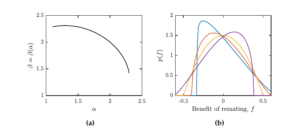
In particular, when \(\alpha=\beta=2\), \(f\) follows a symmetric distribution with variance \(1/20\). Using 5, for every \(\alpha\in [1.1,2.3]\), we can use MATLAB’s numerical solver for the cubic equation and find \(\beta=\beta(\alpha)\) such that the shifted \(Beta(\alpha,\beta)\) distribution still has a variance \(1/20\). This is demonstrated in Figure 1 (a). The Figure 1 (b) shows several examples of distributions of \(f\) for different values of \(\alpha\) and \(\beta\).
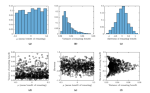
To fully understand the effects of skewness on the optimal toxicity level, we performed the following experiment. We randomly generated over 700 triples \((\mu, \alpha, \beta)\) with \(\mu\) uniformly distributed in \([-0.5,0.5]\) and \(\alpha\) and \(\beta\) uniformly distributed in \([0.5]\). For each such a triple, we recorded the remating benefits mean (\(\mu\)), variance (given by formula 5) and skewness (given by formula 6). We numerically found the Nash equilibria for each of the triples. Figure 2 shows the summary of the distribution characteristics (mean, variance and skewness) and their correlations.
The resulting outcomes were then analyzed for the effects of the mean, variance and skewness using the Partial Rank Correlation Coefficient (PRCC) scheme [9,10]. The partial rank correlation coefficient between model parameter \(p\) and model output \(o\) is given by \[r_{R_p,R_o} = \frac{\text{Cov}(R_p,R_o)}{\sqrt{\text{Var}(R_p)\text{Var}(R_o)}}, \tag{7}\] where \(R_p\) and \(R_o\) are residuals of the rank-transformed linear regression models for \(p\) and \(o\); see, for example, [2] for more details. A PRCC value of \(\pm1\) means a perfectly linear relationship while a PRCC value of 0 means no linear relationship. We used the matlab implementation adapted from [11].
To find Nash equilibria, we have to look for the best responses, i.e., for every \(t\), we find \(BR(t)\) such that \(w\big(BR(t),t)\geq w(t',t)\) for all \(t'\). The strategy is Nash equilibrium if it is the best response itself, i.e., \(t_{NE}=BR(t_{NE})\). Not every Nash equilibrium can be achieved by natural selection. We will look for those that are continuously stable [12], i.e., when the majority slightly deviates from it, some reduction of this deviation becomes individually advantageous. This means that \(\frac{d}{dt}BR(t)<0\).
To implement the search for continuously stable Nash equilibria numerically, we used MATLAB. We selected a mesh of \(N=101\) uniformly distributed points \(t_n = (n-1)*0.01 \in[0,1]\) for \(n=0,1, \ldots, N\). For every \(n\) and \(n'\), we calculate \(w(t_{n'},t_n)\) based on the formula 2 using MATLAB’s built-in functions pdf to generate the probability distribution function and integral to calculate the integrals in (2). For every \(n\), we then found \(n'=br(n)\), such that \(t_{n'}\) is the best response to \(t\) in our mesh, i.e., \[w(t_{n'}, t_n) \geq w(t_k, t_n), \text{ for all $k$}. \tag{8}\]
Finally, we identified all values of \(n^*\) where \(br(n)\) “crosses” the diagonal line, i.e., where \(n-br(n)\) switches the sign. More specifically, we looked for \(n\) where \(n-br(n)=0\) or where \((n-br(n))((n+1)-br(n+1))<0\). Moreover, we classified those equilibria as continuously stable if the sign switch was from non-negative to negative. The equilibrium was not continuously stable if the sign switch was from non-positive to positive. The reason we were identifying the points where the sign switches rather than exact roots of \(BR(t) = t\) is that sometimes the roots did not exist for our mesh.
We note that [3] used a little more sophisticated approach to identify the Nash equilibria. First, they looked for the local maxima of \(w(\cdot, t)\) by solving for roots of the derivative with respect to the first coordinate and then they checked whether the roots are absolute maxima and continuously stable strategies. However, when we tried to replicate this approach, we had trouble identifying all solutions (and then we had to resort to a similar procedure as described above).
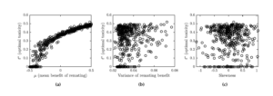
Figure 3 shows how the optimal toxicity level depends on the mean benefit of remating for various shape parameters \(\alpha\) and \(\beta\). Most notably, there is a region with \(|\mu|\) small enough for which there is only one NE with \(t^*>0\); this NE is also continuously stable. When \(|\mu|\) is large enough and \(\mu\) is negative, then the non-toxic is the only NE and it is also continuously stable. When \(\mu>0\) is large enough then there are two continuously stable toxicity levels – one positive and one \(0\). There is also another NE with positive toxicity, but that is not stable. For “medium” values of \(|\mu|\), the non-toxic equilibrium is not continuously stable. Figure 3 also illustrates that qualitatively the model predictions do not depend on skewness.

Figure 4 shows how the optimal toxicity level depends on the characteristics of the distributions. It follows that the mean of the distribution has the biggest effect and the optimal toxicity could be mean alone.
The variance and skewness do have an effect too, though. This is demonstrated by the values of partial rank correlation coefficients shown in Figure 5. The effect of the variance is weaker than the effect of the mean; the effect of skewness is the weakest of the three.
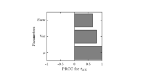
Figure 6 demonstrates the effect of the asymmetry when the mean and the variance are fixed. We can see that for most part, increasing the skewness increases the optimal toxicity. Nevertheless, the effect is more complicated and there is a threshold skewness level \(s_0\) such that the toxicity level is decreasing when the skewness is larger than \(s_0\).
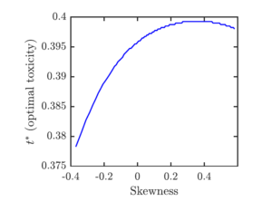
We investigated the effects of (a)symmetry on the optimal toxin allocation. In most instances, increasing skewness of the distribution of remating benefits resulted in increasing the optimal toxicity. This increase was much smaller than the increase resulting from increasing the distribution mean. Such a result is perhaps not surprising as the skewness depends on the third moments of the distribution while the mean depends on the first moment. Nevertheless, we also saw that the increase in skewness may result in a small decrease in toxicity when the skewness is already high enough.
We have adopted beta distributions as they allowed us to naturally and quickly vary the skewness and other characteristics of the distribution as necessary. However, other kinds of distributions would be possible, including triangular distribution which would also account for various asymmetries.
We have also studied only one specific biological problem. It is entirely possible that the outcomes of the other models would depend on the symmetry of the distribution in a much more crucial way.
Villaverde, A. F. (2022). Symmetries in dynamic models of biological systems: Mathematical foundations and implications. Symmetry, 14(3), 467. MDPI.
Marino, S., Hogue, I. B., Ray, C. J., & Kirschner, D. E. (2008). A methodology for performing global uncertainty and sensitivity analysis in systems biology. Journal of Theoretical Biology, 254(1), 178–196. Elsevier.
Johnstone, R. A., & Keller, L. (2000). How males can gain by harming their mates: Sexual conflict, seminal toxins, and the cost of mating. The American Naturalist, 156(4), 368–377. The University of Chicago Press.
Rueppell, O., Johnson, N., & Rychtář, J. (2008). Variance-based selection may explain general mating patterns in social insects. Biology Letters, 4(3), 270–273. The Royal Society London.
Oldroyd, B. P., & Fewell, J. H. (2007). Genetic diversity promotes homeostasis in insect colonies. Trends in Ecology & Evolution, 22(8), 408–413. Elsevier.
Maynard Smith, J. (1974). The theory of games and the evolution of animal conflicts. Journal of Theoretical Biology, 47(1), 209–221. Elsevier.
Gupta, A. K., & Nadarajah, S. (2004). Handbook of beta distribution and its applications. CRC Press.
Saltelli, A., Tarantola, S., Campolongo, F., & Ratto, M. (2004). Sensitivity analysis in practice: A guide to assessing scientific models (Vol. 1). Wiley Online Library.
Blower, S. M., & Dowlatabadi, H. (1994). Sensitivity and uncertainty analysis of complex models of disease transmission: An HIV model, as an example. International Statistical Review, 62(2), 229–243. .
Kirschner, D. (2020). Uncertainty and sensitivity functions and implementation. Retrieved from http://malthus.micro.med.umich.edu/lab/usanalysis.html (Accessed: 2024-04-15).
Eshel, I. (1983). Evolutionary and continuous stability. Journal of Theoretical Biology, 103(1), 99–111. Elsevier.
Strassmann, J. (2001). The rarity of multiple mating by females in the social Hymenoptera. Insectes Sociaux, 48, 1–13. Springer.