
The heat equation is a fundamental partial differential equation with wide-ranging applications in diverse scientific and engineering disciplines, including heat transfer, diffusion processes, and financial modeling. Numerical methods are indispensable tools for approximating solutions to this equation, especially when analytical solutions are intractable or unavailable. Numerous numerical schemes have been developed to solve the heat equation, each with its own strengths and weaknesses in terms of accuracy, stability, and computational cost.
This paper focuses on a specific, existing numerical scheme for solving the one-dimensional heat equation. As discussed in [1], parabolic partial differential equations (PDEs) play a crucial role in modeling various physical phenomena, and the Crank-Nicolson scheme is a widely used finite difference method for such PDEs. However, researchers have proposed modifications to the standard Crank-Nicolson scheme to enhance its performance. [1] proposed one such modified Crank-Nicolson scheme with potential benefits for engineering, financial mathematics, and fluid dynamics. While this modified scheme has been proposed, a comprehensive convergence analysis, which rigorously establishes its accuracy and reliability, is often lacking. Previous work, such as [2], has explored numerical evaluation of heat conduction type PDEs, while [3] investigated convergence of finite difference methods under temporal refinement. Other researchers, like [4], have examined convergence for convection-diffusion problems with singular solutions. Furthermore, [5] considered Cauchy problems of nonlinear PDEs using semi-discrete finite difference approximations. Reference [6] investigated the convergence and stability of parabolic PDEs using implicit schemes. While [1] investigated the stability of their modified scheme, a detailed analysis of its convergence properties remains an open area. Therefore, the primary motivation behind this work is to provide a new approach to the derivation of this modified Crank-Nicolson scheme proposed by [1] and to rigorously establish its convergence properties.
This involves a detailed derivation of the local truncation error, which quantifies the error introduced at each time step, and a rigorous stability analysis, which ensures that errors do not grow unboundedly as the computation progresses. Specifically, we propose and prove two theorems related to the local truncation error and consistency of the scheme. Furthermore, we investigate the scheme’s accuracy through step size refinement, observing how the error decreases as the spatial and temporal discretization becomes finer. The stability of the scheme is analyzed using the matrix method. Finally, the performance of the scheme is validated through numerical experiments conducted in a MATLAB environment. We compare the numerical solutions obtained with the scheme to the exact solution, and we examine the L2 norm of the error to assess the overall accuracy and convergence rate. This comprehensive analysis contributes to a deeper understanding of the scheme’s properties and provides a solid foundation for its reliable application.
We consider the parabolic partial differential equation of the form \[\frac{1}{c^{2}}\frac{\partial s}{\partial t} = \frac{\partial ^{2}s}{\partial x^{2}}, \ 0 \leq x \leq l, \ t > 0, \label{eq1} \tag{1}\] with the initial condition \[\frac{s(x, 0)}{s(x)} = 1, \ 0 \leq x \leq l, \label{eq2} \tag{2}\] and the boundary conditions \[\left\{ \begin{array}{cr} s(x, 0)\ \ \ = s(t)\quad 0 < t,\\ s(1, t)\ \ \ = h(t)\quad 0 < t. \end{array} \right. \label{eq3} \tag{3}\]
In Eq. (1) above, \(c^{2}\) is a constant and for the derivation of the scheme, we assume \(c = 1.\)
A rectangular mesh line with domain \(0 \leq x \leq l, \ t > 0,\) is divided into \(D\) equal parts such that, the mesh length on \(x-\)axis is given by \(h = \frac{l}{D}\) and the points on the \(x_{i} = ih,\ i = 0, 1, 2,…M.\) For time \((t)\) axis, we let \(t_{j} = jk,\) then we have the mesh point as \((x_{i}, t_{j})\) where \(t_{j}\) is referred to as the \(j^{th}\) time level. For any point \((x_{i}, t_{j}),\) the numerical and exact solution are given by \(s_{i,j}\) and \(s(x_{i}, t_{j})\) respectively.
The finite difference representation of Eq. (1) incorporates the spatial second derivative, which is approximated using a combination of the current and previous time step. This lead to the development of modified Crank-Nicolson scheme as derived hereunder; Let \(\nabla _t\) be the backward difference operator and let \[k\frac{\partial s}{\partial t} = -\log(1 – \nabla _{t} s) = \left[\nabla _{t} + \frac{1}{2}\nabla _{t}^{2} + \frac{1}{3}\nabla _{t}^{3} + …\right]s , \label{eq4} \tag{4}\] approximating the above gives \[\frac{\partial s}{\partial t} \simeq \left[\nabla _{t} + \frac{1}{2} \nabla _{t}^{2}\right]s, =\left[\frac{\nabla _{t}}{1 – \frac{1}{2}\nabla _{t}}\right]s .\label{eq5} \tag{5}\]
Expanding the operator at the R.H.S gives \[\frac{\partial s}{\partial t} = \nabla _{t}\left[1 – \frac{1}{2}\nabla _{t}\right]^{-1}= \nabla _{t}\left[1 + \frac{1}{2}\nabla _{t} + \frac{1}{4}\nabla _{t}^{2} + …\right]. \label{eq6} \tag{6}\]
Eq. (6) agrees with the first two terms in Eq. (1). Applying the differential equation at the nodal points \((i, j),\) we have \[\left(\frac{\partial s}{\partial t}\right)_{i, j} = c^{2}\left(\frac{\partial ^{2}s}{\partial x^{2}}\right)_{i, j}. \label{eq7} \tag{7}\]
Then from Eq. (5) \[\frac{1}{k} \left[\frac{\nabla _{t}}{1 – \frac{1}{2}\nabla _{t}}\right]s_{i, j} = \frac{c^{2}}{h^{2}}\delta ^{2}_{x}s_{i, j},\label{eq8} \tag{8}\] from where \[\nabla _{t} s_{i, j} = \frac{kc^{2}}{h^{2}}\left(1 – \frac{1}{2}\nabla _{t}\right)\delta ^{2}_{x}s_{i, j},\label{eq9} \tag{9}\] simplifying (9) gives \[= r s_{i, j} (\delta ^{2}_{x}s_{i, j} – \frac{1}{2}\delta ^{2}_{x}\nabla _{t}s_{i, j}), \label{eq10} \tag{10}\] where \(r = \frac{kc^{2}}{h^{2}}\) Eq. (10) can be re-written as \[\nabla _{t}s_{i, j} = r (\delta ^{2}_{x}s_{i, j} – \frac{1}{2}\delta ^{2}_{x}(s_{i, j} – s_{i, j-1})). \label{eq11} \tag{11}\]
Expanding and solving Eq. (11) gives \[\nabla _{t}s_{i, j} = \frac{r}{2} (\delta ^{2}_{x}s_{i, j} + \delta ^{2}_{x}s_{i, j-1}). \label{eq12} \tag{12}\]
Re-arranging and solving Eq. (12) results to \[s_{i, j} – \frac{r}{2} \delta ^{2}_{x} s_{i, j} = s_{i, j-1} + \frac{r}{2} \delta ^{2}_{x}s_{i, j-1},\label{eq13} \tag{13}\] using the fact that \(\delta ^{2}_{x}s_{i, j} = s_{i+1}, j – 2s_{i, j} + s_{i-1, j}\) and substituting into Eq. (13) gives the following scheme \[(1 + r) s_{i, j} – \frac{r}{2} (s_{i+1, j} + s_{i-1, j}) = (1 – r ) s_{i, j-1} + \frac{r}{2}(s_{i+1, j-1} + s_{i-1, j-1}).\label{eq14} \tag{14}\]
Eq. (14) is the modified Crank-Nicolson approximation, which is represented as the following tri-diagonal matrices; \[\begin{bmatrix} 1 + r & -\frac{r}{2} \\ -\frac{r}{2} & 1 + r &-\frac{r}{2} \\ & \ddots \\ & &-\frac{r}{2} & 1 + r & -\frac{r}{2}\\ & & & -\frac{r}{2} & 1 + r \\ \end{bmatrix} \begin{bmatrix} s_{1,j}\\ s_{2,j}\\ s_{3,j}\\ \vdots\\ s_{i-1,j}\\ \end{bmatrix} = \begin{bmatrix} 1 – r & \frac{r}{2} \\ \frac{r}{2} & 1 – r & \frac{r}{2} \\ & \ddots \\ & & \frac{r}{2} & 1 – r & \frac{r}{2}\\ & & & \frac{r}{2} & 1 – r \\ \end{bmatrix} \begin{bmatrix} s_{1,j-1}\\ s_{2,j-1}\\ s_{3,j-1}\\ \vdots \\ s_{i-1,j-1} \end{bmatrix}. \label{eq15} \tag{15}\]
For the local truncation error of the modified Crank-Nicolson scheme, Taylor’s series expansion is employed. To do this, the numerical methods approximation is compared to the exact solution of the differential equations. For the derivation of the local truncation error, the following lemma is used;
Lemma 1. Let \(S(t, x)\) be a continuously differentiable function satisfying the parabolic partial differential Eq. (1). If we approximate the time derivative \(s_{t}\) at a point \((t_{n}, x_{i})\) using a finite difference scheme that involves the value of \(s\) at \((t_{n}, x_{i}),\ (t_{n-1}, x_{i}),\ (t_{n}, x_{n\pm 1}),\) then the truncation error is given by \(T(t_{n}, x_{i}) = \rho D(t_{n}, x_{i}).\) Where \(\rho\) is the step size and \(D(t_{n}, x_{i})\) is a function that depends on the specific finite difference scheme and the derivative of \(s\) up to certain order.
Theorem 1. Let \(s(t,x)\) be a continuously differentiable solution of a parabolic partial differential equation. Let \(s(t_n, x_i)\) represent the exact value of \(s\) at the discrete points \((t_n, x_i)\). If \(\tilde{s}(t_n, x_i)\) denotes the numerical approximation of \(s(t_n, x_i)\) obtained using the modified Crank-Nicolson scheme, then the local truncation error \(T(t_n, x_i)\) at the point \((t_n, x_i)\) is given by \[T(t_n, x_i) = s(t_n, x_i) – \tilde{s}(t_n, x_i).\]
Proof. Given that \(s(t,x)\) is continuously differentiable, the expansion of \(s_{i+1,j-1}\) and \(s_{i-1,j-1}\) gives \[s_{i+1, j-1} = s_{i,j} + \left[h\frac{\partial s}{\partial x} – k\frac{\partial s}{\partial t}\right] + \frac{1}{2}\left[h^2\frac{\partial^2 s}{\partial x^2} – k^2\frac{\partial^2 s}{\partial t^2}\right] + \frac{1}{6}\left[h^3\frac{\partial^3 s}{\partial t^3} – k^3\frac{\partial^3 s}{\partial t^3}\right] + \dots, \label{eq16} \tag{16}\] and \[s_{i-1, j-1} = s_{i,j} – \left[h\frac{\partial s}{\partial x} + k\frac{\partial s}{\partial t}\right] – \frac{1}{2}\left[h^2\frac{\partial^2 s}{\partial x^2} + k^2\frac{\partial^2 s}{\partial t^2}\right] – \frac{1}{6}\left[h^3\frac{\partial^3 s}{\partial t^3} + k^3\frac{\partial^3 s}{\partial t^3}\right] + \dots, \label{eq17} \tag{17}\] and similarly, \[s_{i-1,j} = s(x_i – h, t_j), \label{eq18} \tag{18}\] which can be expanded as \[s_{i-1,j} = s_{i,j} – h\left(\frac{\partial s}{\partial x}\right)_{i,j} + \frac{h^2}{2!}\left(\frac{\partial^2 s}{\partial x^2}\right)_{i,j} – \frac{h^3}{3!}\left(\frac{\partial^3 s}{\partial x^3}\right)_{i,j} + \frac{h^4}{4!}\left(\frac{\partial^4 s}{\partial x^4}\right)_{i,j} – \frac{h^5}{5!}\left(\frac{\partial^5 s}{\partial x^5}\right)_{i,j} + O(h^6), \label{eq19} \tag{19}\] and also, \[s_{i,j+1} = s(x_i, t_j + k), \label{eq20} \tag{20}\] which expands to \[s_{i,j+1} = s_{i,j} + k\left(\frac{\partial s}{\partial t}\right)_{i,j} + \frac{k^2}{2!}\left(\frac{\partial^2 s}{\partial t^2}\right)_{i,j} + \frac{k^3}{3!}\left(\frac{\partial^3 s}{\partial t^3}\right)_{i,j} + \frac{k^4}{4!}\left(\frac{\partial^4 s}{\partial t^4}\right)_{i,j} + \frac{k^5}{5!}\left(\frac{\partial^5 s}{\partial t^5}\right)_{i,j} + \dots + O(k^6). \label{eq21} \tag{21}\]
If \[T_{i,j} = \frac{1}{k}\left(s_{i,j} – s_{i,j-1}\right) – \frac{1}{2h^2}\left(s_{i+1,j-1} – 2s_{i,j-1} + s_{i-1,j-1} + s_{i+1,j} – 2s_{i,j} + s_{i-1,j}\right), \label{eq22} \tag{22}\] substituting the expansions into Eq. (22) and canceling like terms gives \[T_{i,j} = \left(\frac{\partial s}{\partial t}\right) – \left(\frac{\partial^2 s}{\partial x^2}\right) + \left(\frac{k}{2}\frac{\partial^2 s}{\partial t^2} + \frac{h^2}{12}\frac{\partial^4 s}{\partial x^4}\right) + \left(\frac{k^3}{6}\frac{\partial^3 s}{\partial t^3} + \frac{h^4}{720}\frac{\partial^6 s}{\partial x^6}\right),\] or equivalently, \[T_{i,j} = \left(\frac{\partial s}{\partial t} – \frac{\partial^2 s}{\partial x^2}\right) + \left(\frac{k}{2}\frac{\partial^2 s}{\partial t^2} + \frac{h^2}{12}\frac{\partial^4 s}{\partial x^4}\right) + \left(\frac{k^3}{6}\frac{\partial^3 s}{\partial t^3} + \frac{h^4}{720}\frac{\partial^6 s}{\partial x^6}\right).\] Truncating terms of \(O(h^6)\) gives \[\frac{\partial s}{\partial t} – \frac{\partial^2 s}{\partial x^2} = 0,\] and at the mesh point \((ih, jk)\), the truncation error is \(O(h^2 + k^2)\). ◻
Consistency of a finite difference approximation implies that; as the grid is refined \(((h, k \rightarrow \infty\))) then the truncation error also tends to zero.
If the truncation error \(T_{i,j}(S)\) at the mesh point \((ih, jk)\) is defined by \[S_{i,j} = D_{i,j}(S) – L(S_{i,j}), \label{eq23} \tag{23}\] then as \(T_{i,j}(s)\) tends to zero as \(h,k \rightarrow 0,\) then the scheme is said to be consistent with the partial differential equation.
Next is the prove of the consistency of the scheme.
Theorem 2. Let \(s(x, t)\) be a continuously differentiable solution of the parabolic partial differential equation (2). The modified Crank–Nicolson scheme approximates \(s_t\) using a discretized form. If the local truncation error \(T(t_n, x_n) \to 0\) as \(\Delta t, \Delta x \to 0\), then the scheme is consistent with the parabolic differential equation.
Proof. Let \(L_{i,j}(S) = 0\) from Eq. (23), then \[\label{eq24} T_{i,j}(S) = D_{i,j}(S). \tag{24}\]
This shows that the local truncation error coincides with the discretization error. Hence, \[\label{eq25} T_{i,j}(S) = D_{i,j}(S) \to \left( \frac{\partial s}{\partial t} – \frac{\partial^2 s}{\partial x^2} \right) + \left( \frac{k}{2} \frac{\partial^2 s}{\partial t^2} + \frac{h^2}{12} \frac{\partial^4 s}{\partial x^4} \right) + \left( \frac{k^3}{6} \frac{\partial^3 s}{\partial t^3} + \frac{h^4}{720} \frac{\partial^6 s}{\partial x^6} \right) + \cdots \tag{25}\]
If \(k = r h\), then \[\label{eq26} D_{i,j}(S) = \left( \frac{\partial s}{\partial t} – \frac{\partial^2 s}{\partial x^2} \right) + \left( \frac{r h}{2} \frac{\partial^2 s}{\partial t^2} + \frac{h^2}{12} \frac{\partial^4 s}{\partial x^4} \right) + \left( \frac{(r h)^3}{6} \frac{\partial^3 s}{\partial t^3} + \frac{h^4}{720} \frac{\partial^6 s}{\partial x^6} \right) + \cdots \tag{26}\]
Taking the limit as \(h \to 0\), we get \[\label{eq27} \lim_{h \to 0} D_{i,j}(S) = \lim_{h \to 0} \left[ \left( \frac{\partial s}{\partial t} – \frac{\partial^2 s}{\partial x^2} \right) + \left( \frac{r h}{2} \frac{\partial^2 s}{\partial t^2} + \frac{h^2}{12} \frac{\partial^4 s}{\partial x^4} \right) \right], \tag{27}\] \[\label{eq28} \Rightarrow \frac{\partial s}{\partial t} – \frac{\partial^2 s}{\partial x^2} = 0. \tag{28}\]
Similarly, if \(k = r h^2\), we obtain \[\label{eq29} D_{i,j}(S) = \left( \frac{\partial s}{\partial t} – \frac{\partial^2 s}{\partial x^2} \right) + \left( \frac{r h^2}{2} \frac{\partial^2 s}{\partial t^2} + \frac{h^2}{12} \frac{\partial^4 s}{\partial x^4} \right) + \cdots, \tag{29}\] and hence \[\label{eq30} \lim_{h \to 0} \left[ \left( \frac{\partial s}{\partial t} – \frac{\partial^2 s}{\partial x^2} \right) + \left( \frac{r h^2}{2} \frac{\partial^2 s}{\partial t^2} + \frac{h^2}{12} \frac{\partial^4 s}{\partial x^4} \right) \right] + \cdots, \tag{30}\] gives \[\label{eq31} \frac{\partial s}{\partial t} – \frac{\partial^2 s}{\partial x^2} = 0. \tag{31}\]
Eq. (31) confirms that the scheme is consistent. The next step would be to investigate the stability of the scheme, which is a necessary condition for convergence. ◻
The matrix in Eq. (15) can be rewritten as \[(2I_{N-1} – rT_{N-1}) s_{i} = (2I_{N-1} + rT_{N-1}) s_{i-1}, \label{eq32} \tag{32}\] where \(T_{N-1}\) is a tridiagonal matrix. From Eq. (32), we obtain \[s_{i} = (2I_{N-1} – rT_{N-1})^{-1}(2I_{N-1} + rT_{N-1}) s_{i-1},\] which can be expressed as \[s_{i} = \frac{2I_{N-1} + rT_{N-1}}{2I_{N-1} – rT_{N-1}} s_{i-1}. \label{eq33} \tag{33}\]
Let \[\mathcal{D} = \frac{2I_{N-1} + rT_{N-1}}{2I_{N-1} – rT_{N-1}}, \label{eq34} \tag{34}\] so that from Eq. (33), we have \[s_{i} = \mathcal{D} s_{i-1}, \label{eq35} \tag{35}\] where \(\mathcal{D}\) is a tridiagonal matrix. The eigenvalues \(\lambda_i\) of \(\mathcal{D}\) are given by \[\lambda_{i} = a + 2\sqrt{bc} \cos \left( \frac{i\pi}{N+1} \right), \label{eq36} \tag{36}\] and by solving for \(\lambda_i\) using Eq. (33), we obtain \[\lambda_{i} = \frac{2 + 4r \sin^2 \left( \frac{i\pi}{2N} \right)}{2 – 4r \sin^2 \left( \frac{i\pi}{2N} \right)}. \label{eq37} \tag{37}\]
Therefore, the norm of \(\mathcal{D}\) is given by \[\| \mathcal{D} \| = \lambda_{\max}(\mathcal{D}) = \max \left| \frac{1 – 2r \sin^2 \left( \frac{i\pi}{2N} \right)}{1 + 2r \sin^2 \left( \frac{i\pi}{2N} \right)} \right| < 1, \quad \forall\, r > 0, \label{eq38} \tag{38}\] which shows that the modified scheme is unconditionally stable.
Theorem 3 (Lax-Richtmyer’s theorem [7]). If a linear finite difference equation is consistent with a properly posed linear initial value problem then stability guarantees convergence.
Following the statement of the Lax-Richtymer’s theorem, it is sufficient enough that the scheme is convergent having shown it is consistent and unconditionally stable. But we shall use the following definition of convergence to show numerically that the scheme is convergent.
Definition 1. (Convergence [8]) A finite difference approximation is said to be convergent if \[\xi _{i,j} = ||\bar{s}_{i,j} – s_{i,j}||\rightarrow 0\ as\ h, k \rightarrow 0,\label{eq39} \tag{39}\] where \(\xi _{i,j}\) is the error, \(\bar{s}_{i,j}\) is the analytical solution and \(s_{i,j}\) is the numerical solution.
As the grid size (or time step) decreases, the numerical solution approaches the exact solution. Test for convergence, shall be based on the fact that ” if comparing the solutions by calculating the difference between corresponding grid points on the coarse and refined grid, the difference decreases as the grid is refined then convergence is certain”. That is, it indicate convergence.
This section presents some numerical examples to verify the convergence of the scheme using the above definition:
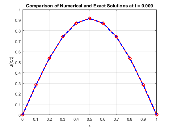
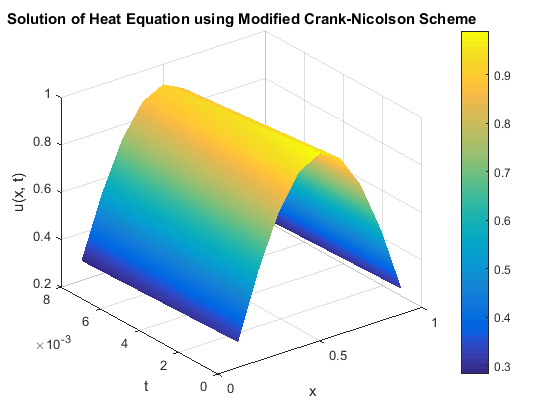
Experiment 1. Consider the following parabolic partial differential equation \[\frac{\partial s}{\partial t} = \frac{\partial ^{2}s}{\partial x^{2}},\ \ 0 < x < 1 ,\label{eq40} \tag{40}\] subjected to the initial condition \[\frac{s(x, 0)}{\sin \pi x} = 1, \ 0 \leq x \leq 1 ,\label{eq41} \tag{41}\] and the boundary conditions \[\left\{ \begin{array}{cr} s(x, 0)= 0, \ \quad 0 < t,\\ s(1, t)= 0, \ \quad 0 < t. \end{array} \right. \label{eq42} \tag{42}\] The solution is given by \[s(x, t) = e^{-\pi ^{2}t}\sin (\pi x).\] We investigate its convergence using \(h = 0.1,\) and \(r = 0.05.\) Equation (40) together with the initial and boundary conditions (41) and (42), when solved using Equation (15), results in a tri-diagonal matrix with the results presented in Table 1. The accuracy of the numerical method is further evaluated by comparing it with the exact solution at \(x = 0.5\) for various time values, as shown in Table 2. This comparison highlights the minimal errors and low percentage errors, demonstrating the effectiveness of the modified Crank–Nicolson scheme. Figure 1 presents a graphical comparison of the numerical and exact solutions, illustrating their close agreement. Figures 2 and 5 provide visual representations of the numerical solution to the heat equation, reinforcing the accuracy and reliability of the implemented scheme.
| \(t\) | \(x\) | \(j\) | \(s_{1,\ j}\) | \(s_{2,\ j}\) | \(s_{3,\ j}\) | \(s_{4,\ j}\) | \(s_{5,\ j}\) | \(s_{6,\ j}\) | \(s_{7,\ j}\) | \(s_{8,\ j}\) | \(s_{9,\ j}\) |
|---|---|---|---|---|---|---|---|---|---|---|---|
| 0.001 | 0.1 | 1 | 0.3060 | 0.5821 | 0.8011 | 0.9418 | 0.9903 | 0.9418 | 0.8011 | 0.5821 | 0.3060 |
| 0.002 | 0.2 | 2 | 0.3030 | 0.5764 | 0.7933 | 0.9326 | 0.9806 | 0.9326 | 0.7933 | 0.5764 | 0.3030 |
| 0.003 | 0.3 | 3 | 0.3001 | 0.5708 | 0.7856 | 0.9235 | 0.9711 | 0.9235 | 0.7856 | 0.5708 | 0.3001 |
| 0.004 | 0.4 | 4 | 0.2972 | 0.5652 | 0.7780 | 0.9145 | 0.9616 | 0.9145 | 0.7780 | 0.5652 | 0.2972 |
| 0.005 | 0.5 | 5 | 0.2943 | 0.5597 | 0.7704 | 0.9056 | 0.9522 | 0.9056 | 0.7704 | 0.5597 | 0.2943 |
| 0.006 | 0.6 | 6 | 0.2914 | 0.5543 | 0.7629 | 0.8968 | 0.9430 | 0.8968 | 0.7629 | 0.5543 | 0.2914 |
| 0.007 | 0.7 | 7 | 0.2886 | 0.5489 | 0.7554 | 0.8881 | 0.9338 | 0.8881 | 0.7554 | 0.5489 | 0.2886 |
| 0.008 | 0.8 | 8 | 0.2857 | 0.5435 | 0.7481 | 0.8794 | 0.9247 | 0.8794 | 0.7481 | 0.5435 | 0.2857 |
| 0.009 | 0.9 | 9 | 0.2830 | 0.5382 | 0.7408 | 0.8709 | 0.9157 | 0.8709 | 0.7408 | 0.5382 | 0.2830 |
| \(t\) | Modified Crank-Nicolson scheme | Exact solutions | Errors | Percentage error |
|---|---|---|---|---|
| 0.005 | 0.9522 | 0.9518 | \(4 \times 10^{-4}\) | 0.04 |
| 0.006 | 0.9430 | 0.9425 | \(5 \times 10^{-4}\) | 0.05 |
| 0.007 | 0.9338 | 0.9332 | \(6 \times 10^{-4}\) | 0.06 |
| 0.008 | 0.9247 | 0.9241 | \(6 \times 10^{-4}\) | 0.06 |
| 0.009 | 0.9157 | 0.9241 | \(6 \times 10^{-4}\) | 0.06 |
Experiment 2. Using a refined mesh of \(h = 0.05,\ k = 0.0005\) such that \(r = 0.2\) present the solution matrix of the problem in Experiment 1 above.
The solution matrix of Experiment 1 together with the initial and boundary conditions using the mesh size \(h = 0.05\) and \(r = 0.1\) is given below for \(1 \leq i \leq 19\) at \(j=1\): \[\begin{bmatrix} 1.2 & -0.1 & 0 & 0& \cdots& \cdots & 0 \\ -0.1 & 1.2 & -0.1 & \ddots & \ddots & \cdots & 0 \\ 0 & -0.1 & 1.2 & -0.1 & \ddots & \cdots & 0\\ \vdots & \vdots & \vdots & \ddots &\ddots & \vdots & \vdots\\ 0 & 0 & 0 & 0 & \ddots & \cdots & 0\\ 0 & 0 & 0 & 0 & \ddots & \cdots & 0\\ 0 & 0 & 0 & 0 & \ddots & \cdot& 0\\ \vdots & \vdots &\vdots & \vdots & \ddots & \ddots & \vdots\\ 0 & 0 & 0 & \cdots & \ddots & -0.1 & 1.2 \\ \end{bmatrix} \begin{bmatrix} s_{1,1}\\ s_{2,1}\\ s_{3,1}\\ s_{4,1}\\ s_{5,1}\\ \vdots \\ \vdots \\ s_{18,1} \\ s_{19,1}\\ \end{bmatrix} = \begin{bmatrix} 0.1557\\ 0.3075\\ 0.4518\\ 0.5849\\ 0.7036\\ 0.8050\\ 0.8866\\ 0.9464\\ 0.9828\\ 0.9951\\ \vdots\\ \vdots\\ 0.3075\\ 0.1557\\ \end{bmatrix},\]
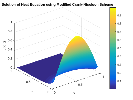
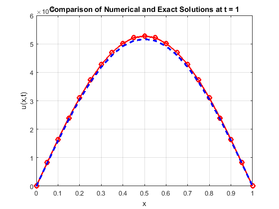
The solutions of the matrix above and the subsequent steps for \(1 \leq i \leq 20\) and \(2 \leq j \leq 19\) are presented in Table 3. Figure 4 shows a comparison graph, while Figures 5 and 6 respectively illustrate the solution of the heat equation and the L2-norm graph.
| \(t\) | \(x\) | \(j\) | \(s_{1,\ j}\) | \(s_{2,\ j}\) | \(s_{3,\ j}\) | \(s_{4,\ j}\) | \(s_{5,\ j}\) | \(s_{6,\ j}\) | \(s_{7,\ j}\) | \(s_{8,\ j}\) | \(s_{9,\ j}\) |
|---|---|---|---|---|---|---|---|---|---|---|---|
| 0.0001 | 0.05 | 1 | 0.1549 | 0.3060 | 0.4495 | 0.5520 | 0.7002 | 0.8011 | 0.8823 | 0.9417 | 0.9780 |
| 0.0002 | 0.10 | 2 | 0.1541 | 0.3045 | 0.4473 | 0.5792 | 0.6967 | 0.7972 | 0.8779 | 0.9371 | 0.9732 |
| 0.0003 | 0.15 | 3 | 0.1534 | 0.3030 | 0.4451 | 0.5763 | 0.6933 | 0.7932 | 0.8736 | 0.9325 | 0.9684 |
| 0.0004 | 0.20 | 4 | 0.1526 | 0.3015 | 0.4429 | 0.5735 | 0.6899 | 0.7855 | 0.8651 | 0.9234 | 0.9589 |
| 0.0005 | 0.25 | 5 | 0.1519 | 0.3000 | 0.4408 | 0.5707 | 0.6865 | 0.7855 | 0.8651 | 0.9234 | 0.9589 |
| 0.0006 | 0.30 | 6 | 0.1511 | 0.2985 | 0.4386 | 0.5679 | 0.6831 | 0.7816 | 0.8608 | 0.9188 | 0.9542 |
| 0.0007 | 0.35 | 7 | 0.1504 | 0.2971 | 0.4365 | 0.5651 | 0.6798 | 0.7778 | 0.8566 | 0.9143 | 0.9495 |
| \(t\) | \(x\) | \(j\) | \(s_{10,\ j}\) | \(s_{11,\ j}\) | \(s_{12,\ j}\) | \(s_{13,\ j}\) | \(s_{14,\ j}\) | \(s_{15,\ j}\) | \(s_{16,\ j}\) | \(s_{17,\ j}\) | \(s_{18,\ j}\) | \(s_{19,\ j}\) |
|---|---|---|---|---|---|---|---|---|---|---|---|---|
| 0.0008 | 0.40 | 8 | 0.9902 | 0.9780 | 0.9417 | 0.8823 | 0.8011 | 0.7002 | 0.5820 | 0.4495 | 0.3060 | 0.1549 |
| 0.0009 | 0.45 | 9 | 0.9853 | 0.9732 | 0.9371 | 0.8779 | 0.7972 | 0.6967 | 0.5792 | 0.4473 | 0.3045 | 0.1541 |
| 0.0010 | 0.50 | 10 | 0.9805 | 0.9684 | 0.9325 | 0.8736 | 0.7932 | 0.6933 | 0.5763 | 0.4451 | 0.3030 | 0.1534 |
| 0.0011 | 0.55 | 11 | 0.9757 | 0.9637 | 0.9279 | 0.8693 | 0.7893 | 0.6899 | 0.5735 | 0.4429 | 0.3015 | 0.1526 |
| 0.0012 | 0.60 | 12 | 0.9709 | 0.9589 | 0.9234 | 0.8651 | 0.7855 | 0.6865 | 0.5707 | 0.4408 | 0.3000 | 0.1519 |
| 0.0013 | 0.65 | 13 | 0.9661 | 0.9542 | 0.9188 | 0.8608 | 0.7816 | 0.6831 | 0.5679 | 0.4386 | 0.2985 | 0.1511 |
| 0.0014 | 0.70 | 14 | 0.9614 | 0.9495 | 0.9143 | 0.8566 | 0.7778 | 0.6798 | 0.5651 | 0.4365 | 0.2871 | 0.1504 |
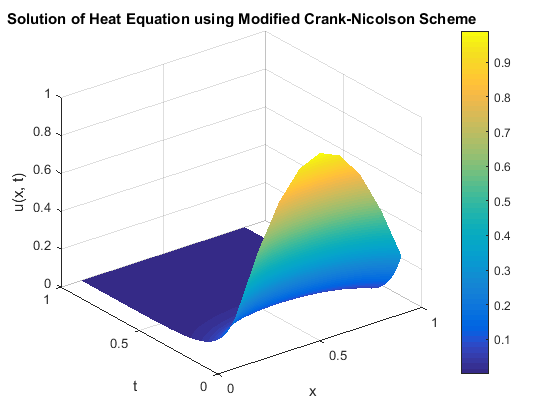
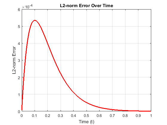
Tables 1 and 2 present the results obtained using the modified Crank-Nicolson scheme to solve the one-dimensional heat equation. These results demonstrate the scheme’s effectiveness and efficiency for solving one-dimensional parabolic equations. Tables 3 show the results of a mesh refinement study for Experiment 1. The data clearly indicate a fast convergence rate, which is also visually confirmed by the accompanying convergence graph. Implementation of the scheme in a MATLAB environment further validates its performance, demonstrating consistency and good agreement with the analytical solutions. The method exhibits improved accuracy, requiring the solution of a tri-diagonal system at each time level. As the step sizes h and k are reduced, the L2-norm error graph initially shows a peak followed by a decay. This suggests that the error initially increases, likely due to the influence of the initial condition, reaches a maximum, and subsequently decreases, indicating an initial accumulation of error followed by stabilization of the numerical scheme. The graph further reveals that the error approaches zero as t tends to 1, implying a close match between the numerical and exact solutions at longer times. This behavior suggests the scheme’s high efficiency.
The results demonstrate that the modified scheme provides accurate approximate solutions and exhibits faster convergence compared to other implicit schemes reported in the literature. The close agreement between the analytical and numerical solutions confirms rapid convergence, consistent with the established definition of convergence, and validates the effectiveness of the scheme. The data presented in Tables 3 further support the scheme’s stability and demonstrate its convergence as the mesh size approaches zero.