
For the basic terminology and notions of graph theory see [1]. Recall that the distance between two vertices \(v_i\) and \(v_j\) of \(G\), denoted by \(d_G(v_i,v_j)\), is the length of the shortest path joining them. The empty graph (edgeless graph) of order \(n \geq 1\) will be denoted by, \(\mathfrak{N}_n\). The notion of exact deg-centric graphs of simple graphs was introduced in [2]. Recall the definition of an exact deg-centric graph from [2].
Definition 1. [2] The exact deg-centric graph of a simple graph \(G\) is the graph \(G_{ed}\) with \(V(G_{ed}) = V(G)\) and \(E(G_{ed}) = \{v_iv_j: d_G(v_i,v_j) = deg_G(v_i)\}\).
From the definition of the exact deg-centric graph of a graph \(G\) it follows that, if the addition of an edge \(v_iv_j\) in \(G_{ed}\) is possible, the addition of the edge \(v_jv_i\) in \(G_{ed}\) is not necessarily possible. Furthermore, if \(\forall~v_i \in V(G)\) the distance \(d_G(v_i,v_j) \neq deg_G(v_i), \forall j\) then \(G_{ed}\) is an empty graph. The interest of the notion of exact deg-centric graphs lies mainly in enlarging the scope of the established study of graphs from graph. Note that obtaining the exact deg-centric graph of any graph (including a disconnected graph) is possible. However, for disconnected graphs the convention is to apply Defifinition 1 componentwise.
Recall that a dominating set in a graph \(G\) with vertex set \(V(G)\) is a set \(S\) of vertices of \(G\) such that every vertex in \(V(G)-S\) is adjacent to at least one vertex in \(S\). The domination number of \(G\), denoted by \(\gamma(G)\), is the minimum cardinality of a dominating set of \(G\). A dominating set of \(G\) of cardinality \(\gamma(G)\) is called a \(\gamma(G)\)-set, [3– 5]. The importance of domination in graphs and the applications thereof have been widely studied.
Recent developments in graph theory have introduced advanced parameters such as the fault-tolerant mixed metric dimension [6], local edge partition dimension [7], mixed partition dimension [8], and face metric dimension [9], which strengthen the framework for vertex and edge identification. These concepts have real-world relevance, especially in nanostructures like V-Phenylenic nanotubes [10] and polyomino-based graphs studied under magic labeling [11]. Studying these advanced parameters for the exact deg-centric graphs of nanostructures is deemed both worthy and important in the field of mathematical chemistry.
The family of linear Jaco graphs (for brevity, Jaco graphs) was introduced by Kok et al. in 2014. Readers are referred to [14] and the references thereto. Also, Assous et al. remarked in [12] that posets of minimal type are related to the notion of Jaco graphs. Note that Jaco graphs are inherently directed graphs. Recall the definitions of Jaco graphs from [13].
Definition 2. [13] The infinite Jaco Graph \(J_\infty(x),\) \(x \in \Bbb N\) is defined by \(V(J_\infty(x)) = \{v_i: i \in \Bbb N\}\), \(A(J_\infty(x)) \subseteq \{(v_i, v_j): i, j \in \Bbb N, i< j\}\) and \((v_i,v_ j) \in A(J_\infty(x))\) if and only if \(2i – d^-(v_i) \geq j.\)
Definition 3. [13] The family of finite Jaco Graphs is defined by \(\{J_n(x) \subseteq J_\infty(x):n,x\in \Bbb N\}.\) A member of the family is referred to as the Jaco Graph, \(J_n(x).\)
Linear Jaco graphs are a fairly new addition to graph theory It represents an infinite family of graphs and the study thereof intersects with amongst others, number theory (specifically with Fibonacci and Lucas number theory, integer sequences in graphs) and modern algebra. In this paper the interest lies with the underlying Jaco graph. Hence, we consider an undirected Jaco graph. Therefore, we shall present an alternative construction method to obtain the family of underlying Jaco graphs.
Construction method to obtain \(J_n(x)\):
(a) Let \(X = \{v_i: i = 4,5,6,\dots,n\}\) and let \(G_2 = P_3 \cup \mathfrak{N}_{n-3}\) where, \(V(\mathfrak{N}_{n-3}) = X\).
(b) By normal consecutive step-count for \(i = 3,4,5,\dots, n-1\) do as follows:
To obtain \(G_i\) add the edges \(v_iv_{i+1}\), \(v_iv_{i+2}\),\(\dots, v_iv_{i+t}\) with \(t\) a maximum such that, \(deg_{G_i}(v_i) \leq i\).
(c) After completion of step-count \(i = n-1\) label the resultant graph, \(J_n(x)\).
Note that \(J_n(x)\) is a simple graph. To clarify the construction method the reader is encouraged to reconstruct the example below.
Since both, Jaco graphs and the notion of exact deg-centric graph from a graph received attention in the literature the authors deem it worthy to contribute by studying firstly, the domination number of a Jaco graph, secondly, studying the exact deg-centric graph of Jaco graphs, thirdly, to find the domination number of \(J_n(x)_{ed}\), \(n \geq 1\) and finally, to consider the complement graphs.
For the purpose of this section we write the open neighborhood of \(v_i\) in a given \(J_n(x)\) as:
\[N(v_i) = N^-(v_i) \cup N^+(v_i),\] where, \(N^-(v_i) = \{v_j:j < i\) and the edge \(v_jv_i\) exists (by definition)\(\}\) and \(N^+(v_i) = \{v_j:j > i\) and the edge \(v_iv_j\) exists (by definition)\(\}\).
Also let \[t_1(v_i) = |N^-(v_i)|\text{ and }t_2(v_i) = |N^+(v_i)|.\]
Note that as \(n\) increase through the consecutive step-count \(1,2,3,\dots\) the \(max\{t_1(v_i):\forall~n \geq i\} = t_1(v_i)\) is obtained in any Jaco graph \(J_n(x)\) which contains the vertex \(v_i\). The same does not necessarily hold for \(max\{t_2(v_i)\) in \(J_n(x):\forall~n \geq i\}\). Professor Stephan Wagner1 identified that, in accordance with sequence A060144 in \(www.oeis.org\) the result \(t_1(v_i) = \lfloor \frac{2(i+1)}{3+\sqrt{5}}\rfloor\) holds. Therefore, for a minimum sufficiently large \(n\),
\(t^\star_2(v_i) = max\{t_2(v_i)\) in \(J_n(x):n\geq m\} = i – \lfloor \frac{2(i+1)}{3+\sqrt{5}}\rfloor,\)
in all Jaco graphs of order, at least \(n\). We now state a trivial claim which requires no further proof.
Claim 1. If two complete graphs, \(K_n\), \(K_m\), \(n \geq 1\), \(m \geq 2\) share one common vertex \(v_i\) then, \(\{v_i\}\) is a minimum dominating set. Note that \(m = 1\) is permissible but redundant.
Notation: For a vertex \(v_i \in V(J_n(x))\) we denote, \(v^\star_i = v_{i+ t^\star_2(v_i)}\). For example, \(v^\star_1 = v_{1+ t^\star_2(v_1)} = v_2\), \(v^\star_2 = v_{2+ t^\star_2(v_2)} = v_3\), and \(v^\star_4 = v_{4+ t^\star_2(v_4)} = v_7\), \(v^\star_7 = v_{7+ t^\star_2(v_7)} = v_{11}\). Using the new notation the vertex set of a Jaco graph can be written as: \[\begin{aligned} V(J_n(x)) =& \{v_1,v_2,v_3\} \cup \{v_4,v_5,v_6,v_7,\dots,v_{11}\} \cup \{v_{12},\dots,\underbrace{v_{12+ t^\star_2(v_{12})}}_{=v^\star_{12}},\dots,v^\star_{12+ t^\star_2(v^\star_{12})}\} \cup \cdots \cup R \\ =& \{v_1,v_2,v_3\} \cup \{v_4,v_5,v_6,v_7,\dots,v_{11}\} \cup \{v_{12},\dots,v_{20},\dots,v_{32}\} \cup \cdots \cup R, \end{aligned}\] where \(R\) is the set of possible residual vertices at the tail end of \(J_n(x)\). This vertex set representation is called the \(\tau\)-representation. As it will become clear later on, it is safe to state at this stage that the \(\tau\)-representation is a specific partition of the vertex set of a finite linear Jaco graph such that each partition subset say \(X\) besides possible \(R\) contains exactly one dominating vertex in respect of \(X\). This property yields the minimum over minimality of dominating sets. Hence, it ensures obtaining a \(\gamma\)-set.
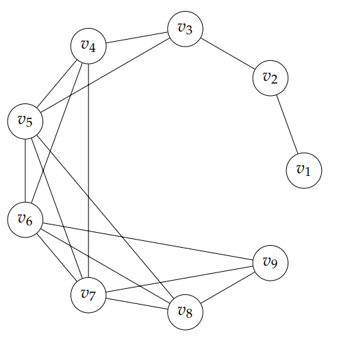
Example 1. From Figure 1 it follows that, \(V(J_9(x)) = \{v_1,v_2,v_3\} \cup \{v_4,v_5,v_6,v_7,v_8,v_9\}\). Since the elements could not run through to contain \(v_{7+ t^\star_2(v_7)} = v_{11}\) we have \(R = \{v_4,v_5,v_6,v_7,v_8,v_9\}\).
Lemma 1. Consider a Jaco graph \(J_n(x)\) and the \(\tau\)-representation:
\(V(J_n(x)) = \{v_1,v_2,v_3\} \cup \{v_4,v_5,v_6,v_7,\dots,v_{11}\} \cup \{v_{12},\dots,\underbrace{v_{12+ t^\star_2(v_{12})}}_{=v^\star_{12}},\dots, v^\star_{12+ t^\star_2(v^\star_{12})}\} \cup \cdots \cup R\).
For brevity the \(\tau\)-representation is written as \(\tau(V(J_n(x)))\). Each of the induced subgraphs:
\(\langle \{v_1,v_2,v_3\}\rangle, \langle \{v_4,v_5,v_6,v_7,\dots,v_{11}\}\rangle, \langle \{v_{12},\dots, \underbrace{v_{12+ t^\star_2(v_{12})}}_{=v^\star_{12}},\dots,v^\star_{12+ t^\star_2(v^\star_{12})}\}\rangle, \cdots \langle R\rangle,\)
has domination number equal to one.
Proof. It is a trivial consequence of Claim 1. Observe that, without loss of generality, the induced subgraph \(\langle \{v_{s},\dots, \underbrace{v_{s+ t^\star_2(v_{s})}}_{=v^\star_{s}},\dots, v^\star_{s+ t^\star_2(v^\star_{s})}\}\rangle\) has a \(\gamma\)-set \(= \{v_{s+ t^\star_2(v_{s})}\}\). Similarly, \(\gamma(\langle R\rangle) = 1\). The result is settled. ◻
Theorem 1. For a given \(J_n(x)\) assume that the \(\tau\)-representation has \(k\) subsets (including \(R\)). Then, \(\gamma(J_n(x)) = k\).
Proof. From Lemma 1 read together with Claim 1 it follows that,
\(\{v_2, v_7,v_{12+ t^\star_2(v_{12})},\dots, v_i \in R\},\)
is a dominating set hence, \(\gamma(J_n(x)) \leq k\). For \(J_3(x)\) it is obvious that there exist the unique \(\gamma\)-set, \(\{v_2\}\). For \(J_4(x)\) it is evident that amongst the options the set \(\{v_2,v_4\}\) is a \(\gamma\)-set. In fact it is trivial to state that \(\{v_2,v_4\}\) is a \(\gamma\)-set of \(J_n(x)\), \(1 \leq n \leq 7\). However, for \(8 \leq n \leq 11\) vertex \(v_4\) can be interchanged with \(v_7\) as an optimal choice. Hence, \(\{v_2,v_7\}\) is a \(\gamma\)-set (not necessarily unique) of \(J_n(x)\), \(1 \leq n \leq 11\). The procedure can be argued as \(n\) increases through to \(12 \leq n \leq 20\) and thereafter as \(n\) increases through \(21 \leq n \leq 32\) and so forth. Suffice to say that, through immediate induction it follows that, \(\gamma(J_n(x)) > k-1\). So the result \(\gamma(J_n(x)) = k\) is settled. ◻
Notation: If \(x = a\) and a new value say, \(b\) has to be allocated to \(x\) the change will be written as \(x \gets b\).
The next heuristic method descibes a method to yield a \(\gamma\)-set \(X\) by identifying a “central” vertex of
each vertex subset in the \(\tau\)-representation (vertex
partitioning). Since the set \(X\) is
of minimum cardinality it follows that, \(\gamma(J_n(x)) = |X|\).
Step 0: Let \(k = 4\), \(j =0\), \(t =
0\) and let set \(X = \{v_2\}\).
Go to Step 1.
Step 1: Calculate \(t^\star_2(v_k) =
k – \lfloor \frac{2(k+1)}{3+\sqrt{5}}\rfloor\) and let \(j \leftarrow k + t^\star_2(v_k)\). If \(n \leq j\) let \(X \gets X \cup \{v_k\}\) and go to Step 4.
If \(n > j\) let \(X \gets X \cup \{v_j\}\) and go to Step
2.
Step 2: Calculate \(t^\star_2(v_j) =
j – \lfloor \frac{2(j+1)}{3+\sqrt{5}}\rfloor\) and let \(t \leftarrow j + t^\star_2(v_j)\). If \(n \leq t\) go to Step 4. If \(n > t\) go to Step 3.
Step 3: Let \(k = t+1\) and go
to Step 1.
Step 4: Let \(\gamma(J_n(x)) =
|X|\) and exit.
Recall the definition of the Fibonacci numbers i.e. \(f_0 = 0\), \(f_1 = 1\) and for \(i \geq 2\), \(f_i = f_{i-1} + f_{i-2}\). For experimental research it is recommended to utilize a Fibonacci number calculator such as the \(\Sigma\)CalculatorSoup\(^\circledR\) Online Fibonacci Calculator. The next lemma requires no proof and is presented as a utility result.
Lemma 2. A direct consequence of the \(\tau\)-representation of the vertex set of \(J_\infty(x)\) is that the set of counting numbers has a similar \(\tau\)-representation i.e.:
\(\mathbb{N} = \{1,2,3\} \cup \{4,5,6,7,8,9,10,11\} \cup \{12,\dots,\underbrace{12 +t^\star_2(12)=20},\dots,\underbrace{20 +t^\star_2(20)=32}\} \cup \cdots.\)
For brevity the \(\tau\)-representation is written as \(\tau(\mathbb{N})\). For the purpose of \(\tau(\mathbb{N})\) we abandon the commutative property of the union of sets and maintain the natural chronological position of each subset say, \(S_1 = \{1,2,3\}\), \(S_2 = \{4,5,6,7,8,9,10,11\}\), \(S_3 = \{12,\dots,12 +t^\star_2(12)=20,\dots, 20 +t^\star_2(20)=32\}\) and so forth.
The next corollary is a direct consequence from the heuristic method read together with Lemma 2.
Corollary 1. Consider the Jaco graph \(J_n(x)\), \(n \geq 1\). If \(n \in S_k\) then,
\(\gamma(J_n(x)) = k\).
Example 2. For \(J_9(x)\) in Figure 1 we have, \(9 \in S_2\). Therefore, \(\gamma(J_9(x)) = 2\).
It is easy to that \(\gamma(J_1(x)_{ed}) = \gamma(J_2(x)_{ed}) = \gamma(J_3(x)_{ed}) = 1\). Computational data (by brute force determination) is tabled below.
Let \(\eta(v_i)=i\). Note that in Table 1 the \(\gamma\)-set for each value \(n \in \mathbb{N}\) has been selected by the criteria that:
\(\sum\limits_{v_i \in \gamma-set}\eta(v_i) = min\left\{\sum\limits_{v_j \in \gamma-set}\eta(v_j):\forall~\gamma\text{-sets}\right\}\).
This criteria is meant to provide a reliable method to identify patterns if such exist, which may lead to provable results or worthy conjectures. The author is currently researching the topic Integer sequences from finite linear Jaco graphs.
| \(i\in{\Bbb{N}}\) | \(t_1(v_i)\) | \(t^\star_2(v_i)\) | \(\gamma(J_n(x)_{ed})\) | \(\gamma\)-set |
|---|---|---|---|---|
| 1=\(f_2\) | 0 | 1 | 1 | \(\{v_1\}\) |
| 2=\(f_3\) | 1 | 1 | 1 | \(\{v_1\}\) |
| 3=\(f_4\) | 1 | 2 | 1 | \(\{v_2\}\) |
| 4 | 1 | 3 | 2 | \(\{v_1,v_2\}\) |
| 5=\(f_5\) | 2 | 3 | 2 | \(\{v_2,v_3\}\) |
| 6 | 2 | 4 | 2 | \(\{v_1,v_3\}\) |
| 7 | 3 | 4 | 2 | \(\{v_2,v_3\}\) |
| 8=\(f_6\) | 3 | 5 | 3 | \(\{v_1,v_2,v_3\}\) |
| 9 | 3 | 6 | 5 | \(\{v_1,v_2,v_3,v_6,v_7\}\) |
| 10 | 4 | 6 | 5 | \(\{v_2,v_3,v_6,v_7,v_8\}\) |
| 11 | 4 | 7 | 5 | \(\{v_2,v_3,v_6,v_7,v_8,\}\) |
| 12 | 4 | 8 | 5 | \(\{v_2,v_3,v_6,v_7,v_8,\}\) |
| 13=\(f_7\) | 5 | 8 | 5 | \(\{v_2,v_3,v_6,v_7,v_8,\}\) |
| 14 | 5 | 9 | 5 | \(\{v_2,v_3,v_6,v_7,v_8,\}\) |
| 15 | 6 | 9 | 6 | \(\{v_1,v_2,v_3,v_6,v_7,v_8,\}\) |
| 16 | 6 | 10 | 8 | \(\{v_1,v_2,v_3,v_6,v_7,v_8,v_{14},v_{15},\}\) |
| 17 | 6 | 11 | 9 | \(\{v_1,v_2,v_3,v_6,v_7,v_8,v_{14},v_{15},v_{16}\}\) |
| 18 | 7 | 11 | 10 | \(\{v_2,v_3,v_6,v_7,v_8,v_{14},v_{15},v_{16},v_{17},v_{18}\}\) |
Convention: For general graphs multiple edges and loops are permitted. By convention the edge \(v_iv_i\) is a loop provided that the graph \(G\) is explicitly classified as a general graph. In simple graphs the edge \(v_iv_i\) is either not permitted or considered to be undefined. The aforesaid is unsatisfactory in many instances. Hence, if a graph \(G\) is explicitly classified as a simple graph the edge \(v_iv_i\) will be defined as an invisible edge within \(v_i\) itself. This convention is sensible because \(K_1\) is the complete graph of smallest order and is connected. The connectedness is compatible with the convention that,
\(\underbrace{\underbrace{K_1}_{complete~graph} \cong \underbrace{\langle \{v_i\}\rangle}_{induced~graph} \equiv \underbrace{v_i}_{vertex} \equiv \underbrace{v_iv_i}_{invisible~edge}}_{Simple~graph}\).
Next, a construction method to obtain \(J_n(x)_{ed}\) is presented. The construction method is cumbersome in that it requires that all \(n\) vertices must be considered in say, consecutive order (not a necessary requirement).
Lemma 3. With reference to \(J_n(x)\), \(n \geq 1\) assume \(deg(v_i) = k\). If a smallest \(j \leq i\) exists such that \(d(v_i,v_j) = k\) then, \(j \in \{1,2,3\}\).
Proof. We will prove the result through induction for only \(v_n\). Hence, for \(deg(v_n) = k = t_1(v_n)\). If the result holds for \(d(v_i,v_j) = t_1(v_i)\) then by implication, either it holds for \(deg(v_i) = k\) in \(J_n(x)\) in general or such \(j \in \{1,2,3\}\) does not exists for \(deg(v_i) = k\). Important though is that the proof technique excludes the absurdity that, “such \(j \in \{1,2,3\}\) does not exist for \(t_1(v_i)\) and such \(j\) does exist for \(deg(v_i)\).”
It is easy to see that the result holds for \(n = 1,2,3,4\). For \(n = 5\) we have \(k = 2\) and \(j = 2\). Hence the result holds for \(n=5\). For \(n = 6\) we have \(k = 2\) and \(j = 3\). Hence the result holds for \(n=6\). Assume that the result holds for \(7 \leq n \leq k\). Consider \(n = k+1\).
Clearly \(t_1(v_{k+1}) > t_1(v_{(k+1)-t_1(v_{k+1})})\). Let \(t_1(v_{k+1}) -1 \geq t_1(v_{(k+1)-t_1(v_{k+1})})\). Then the result holds because it holds for \(v_{(k+1)-t_1(v_{k+1})}\). Hence, if \(j\) exists in respect of vertex \(v_{k+1}\) then \(j \in \{1,2,3\}\). Else, such \(j\) does not exists. By induction the result holds for \(n \geq 1\) at the distance measure \(t_1(v_n)\).
By implied-induction it follows that the main result i.e. if \(deg(v_i) = k\) then, either a smallest \(j \leq i\) and \(j \in \{1,2,3\}\) exists such that \(d(v_i,v_j) = k\) or such \(j\) does not exist, holds for \(n \geq 1\). ◻
A direct consequence of Lemma 3 is that for \(n \geq 4\) the distance in \(J_n(x)_{ed}\), \(d(v_i,v_3) \leq t_1(v_i)\), \(4 \leq i \leq n\). A further direct consequence is put as the next corollary.
Corollary 2. (a) In \(J_n(x)_{ed}\), \(n \geq 2\), \(i \geq 2\) it follows that, \(d(v_i,v_1) \leq i\).
(b) Without loss of generality, if the edge \(v_iv_3\) exists in \(J_n(x)_{ed}\), \(n \geq 4\), \(i \geq 4\) then, the edge \(v_iv_2\) (and not \(v_iv_3\)) exists in \(J_{n+1}(x)_{ed}\). Furthermore, the edge \(v_iv_1\) (and not the edges \(v_iv_2\), \(v_iv_3\)) exists in \(J_{n+2}(x)_{ed}\). Finally, in \(J_{n+3}(x)_{ed}\) a value \(j\) as intended (or meant) in Lemma 3 does not exist for \(v_i\).
Construction method to obtain \(J_n(x)_{ed}\), \(n \geq 2\):
Let \(X = \{v_i: i = 1,2,3,\dots,n\}\). For each \(v_i \in X\) do as follows:
With reference to \(J_n(x)\) assume \(deg(v_i) = k\). Then if it exists,
(a) By Lemma 3, find smallest \(j \leq i\) such that \(d(v_i,v_j) = k\) and add the (dashed) edge \(v_iv_j\) and,
(b) Find greatest (or largest) \(\ell\), \(i \leq \ell\) such that \(d(v_i,v_j) = k-1\). Then add the (solid) edge(s)
\(v_iv_{\ell+1}\), \(v_iv_{\ell+2}\),…,\(v_iv_{\ell+t_2(v_i)}\).
(c) After completion of step-count \(i = n\) label the resultant graph, \(J_n(x)_{ed}\).
Example 3. Figure 2 depicts \(J_9(x)_{ed}\).
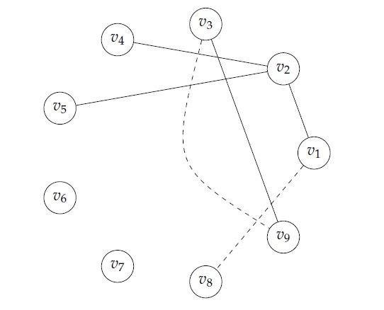
Note that the definition of the exact deg-centric graph of a graph \(G\), implies pseudo orientation. Hence, the edges of \(J_9(x)_{ed}\) are \(v_1v_2\), \(v_2v_4\), \(v_2v_5\), \(v_3v_9\), \(v_8v_1\), \(v_9v_3\). In general the vertex \(v_i\) in an edge \(v_iv_j\), \(i \neq j\) will be called the initiator vertex.
For a given \(J_n(x)_{ed}\) we write the initiated neighborhood of \(v_i\) as:
\[N_{ed}(v_i) = N^-_{ed}(v_i) \cup N^+_{ed}(v_i),\] where, \(N^-_{ed}(v_i) = \{v_j:j < i\) and the edge \(v_iv_j\) exists (by definition)\(\}\) and \(N^+_{ed}(v_i) = \{v_j:j > i\) and the edge \(v_iv_j\) exists (by definition)\(\}\).
Theorem 2. For \(i \in \mathbb{N}\) there exists a minimum \(n \in \{i+1, i+2,i+3\}\) such that, \(N^-_{ed}(v_i) = \emptyset\) in \(J_n(x)_{ed}\).
Proof. The result is a direct consequence of Corollary 2. ◻
A concise description of the exact deg-centric graph of Jaco graphs in general remains elusive. However, three axiom descriptors are important.
Axiom 1. For a sufficiently large \(J_n(x)\) and therefore, a sufficiently large \(J_n(x)_{ed}\):
(a) We have that, \(|N^-_{ed}(v_i)| = 0\) or \(1\) for any \(1 \leq i \leq n\).
(b) There exists an \(i = max\{j: 1 \leq k \leq j, N^-_{ed}(v_k) = \emptyset\}\) for \(n \geq 1\). Furthermore, \(\forall~i+1 \leq q \leq n\) exactly one edge \(v_qv_s\), \(s \in \{1,2,3\}\) exists.
(c) If \(i \geq 1\) and the vertex \(v_i \notin \bigcup\limits_{j<i}N^+_{ed}(v_j)\) then, \(v_i\) is either isolated in \(J_n(x)_{ed}\) or for sufficiently large \(m > n\), \(v_i\) is a root vertex in some tree-subgraph of \(J_m(x)_{ed}\).
Theorem 3. For the Jaco graph \(J_\infty(x)\) the exact deg-centric graph \(J_\infty(x)_{ed}\) is a forest. Put differently, \(\lim\limits_{n\to \infty}J_n(x)_{ed} \to\)forest.
Proof. The proof will follow in two parts. Both parts will follow through immediate induction.
Part 1: Without loss of generality begin with vertex \(v_1\). From Theorem 2 read with Axiom 1 it follows that in \(J_\infty(x)_{ed}\) there exists the tree-subgraph \(T(v_1)\) with edge set,
\(E(T(v_1)) = \{\underbrace{v_1v_2,}\underbrace{v_2v_4,v_2v_5,}\underbrace{v_4v_{19},v_4v_{20},\dots,v_4v_{29},}\underbrace{v_5v_{35},v_5v_{36},\dots,v_5v_{55},}\cdots \}.\)
The root vertex of \(T(v_1)\) is \(v_1\). For brevity, denote \(v_1\dashrightarrow = \underbrace{v_1v_2}\), \(v_2\dashrightarrow = \underbrace{v_2v_4,v_2v_5}\), \(v_4\dashrightarrow = \underbrace{v_4v_{19},v_4v_{20},\dots,v_4v_{29},}\) and so forth.
From observation it follows that the next rooted tree-subgraph is \(T(v_3)\). The edge set is given by,
\(E(T(v_3)) = \{\underbrace{v_3v_9,v_3v_{10},\dots,v_3v_{13},}v_9\dashrightarrow,v_{10}\dashrightarrow,v_{11}\dashrightarrow,\cdots\}.\)
Through immediate induction it follows that tree-subgraphs can be iteratively constructed such that all vertices \(v_i\), \(i \in \mathbb{N}\) are contained in \(V(T(v_1))\cup T(v_3))\cup V(T(v_6)\cup \cdots\). Hence, \(J_\infty(x)_{ed}\) can be decomposed into infinitely many rooted tree-subgraphs each of which is a tree.
Part 2: What remains is to show that a pair of rooted tree-subgraphs with distinct root vertices do not share a common vertex. Let the root vertices of the respective tree-subgraphs be \(v_{r_1} = v_1\), \(v_{r_2} = v_3\), \(v_{r_3} = v_6\), \(v_{r_4},v_{r_5},\dots\). Consider two distinct root vertices say, \(v_{r_i}\), \(v_{r_j}\), \(i > j\). Let \(r_i = r_j + m_1\), \(m_1 \geq 1\). The aforesaid is always possible. From Step (b) in the construction method to obtain \(J_n(x)_{ed}\), \(n \geq 2\) the first distance jumps from vertex \(v_{r_i}\) and vertex \(v_{r_j}\) are to \(v_{r_i+t^\star_2(v_{r_i})}\) and to \(v_{r_j+t^\star_2(v_{r_j})}\), respectively. For the latter two vertices to be a common vertex it must be that \(r_i+t^\star_2(v_{r_i}) = r_j+t^\star_2(v_{r_j})\). Hence, \((r_j + m_1)+t^\star_2(v_{r_i}) = r_j+t^\star_2(v_{r_j})\). Thus, \(m_1+t^\star_2(v_{r_i}) = t^\star_2(v_{r_j})\). Since, \(i > j \Rightarrow r_i > r_j\) the condition \(m_1+t^\star_2(v_{r_i}) = t^\star_2(v_{r_j})\) cannot be satisfied. The condition implies a contradiction to the definition of the general parameter \(t^\star_2(\boxdot)\). By immediate induction it follows that through all iterative distance jumps \(\forall~v_l \in V(J_n(x))\) the contraction holds. Therefore, it follows that any two rooted tree-subgraphs are distinct. This settles the result i.e. the exact deg-centric graph \(J_\infty(x)_{ed}\) is a forest. ◻
A consequence of Theorem 3 is that as \(n\to \infty\) the domination number \(\gamma(J_\infty(x)_{ed})\to \infty\).
Recall that that the complement of a graph \(G\) is defined as the graph, \(\overline{G}\) with \(V(\overline{G}) = V(G)\) and \(E(\overline{G}) = \{v_iv_j: v_iv_j \notin E(G)\}\). Since \(J_n(x)\), \(n = 1,2,3,4\) are paths we only consider the Jaco graphs for \(\geq 5\).
Proposition 1. Let \(n \geq 5\). Then \(\gamma(\overline{J_n(x)}) = 2\).
Proof. Clearly, in \(\overline{J_n(x)}\) the vertex \(v_1\) is adjacent to \(v_j\), \(3 \leq j \leq n\) and \(v_2\) is adjacent to \(v_k\), \(4 \leq k \leq n\). Hence, the vertex subset \(\{v_1,v_2\}\) is a \(\gamma\)-set implying that \(\gamma(\overline{J_n(x)}) \leq 2\). Since \(v_1\) and \(v_2\) are not neighbors we have that, \(\Delta(\overline{J_n(x)}) \neq n-1\). So \(\gamma(\overline{J_n(x)}) > 1\). That settles the result. ◻
Note that for \(n \geq 5\), \(n \neq 6\) the exact deg-centric graph \(J_n(x)_{ed}\) has at least one isolated vertex (or \(K_1\)). By similar reasoning as in the proof of Proposition 1 we state the next corollary.
Corollary 3. Let \(n \geq 5\), \(n \neq 6\). Then \(\gamma((\overline{J_6(x)})_{ed}) = 2\) and \(\gamma((\overline{J_n(x)})_{ed}) = 1\).
Note that the \(\tau\)-representation of the counting numbers \(\mathbb{N}\) read together with Corollary 1 inherently describes an alternative heuristic method to obtain \(\gamma(J_n(x))\), \(n \geq 1\).
Table 1 provides values for both \(\gamma(J_n(x)_{ed})\) and a corresponding \(\gamma\)-set, \(1 \leq n \leq 18\). These values were obtained through computational method. Observe the difficulty in that, the construction of the exact deg-centric graph requires nested-like calculations. For example to find the edge \(v_nv_j\), \(j \in \{1,2,3\}\) if such exists, requires the below.
Claim 2. For the edge \(v_nv_j\), \(j \in \{1,2,3\}\) to exists in \((J_n(x)_{ed})\) it is required that:
\(t_1(v_n) \leq \underbrace{(t_1(v_n) -t_1(v_{n-t_1(v_n)}))-t_1(v_{(t_1(v_n) -t_1(v_{n-t_1(v_n)}))}) – \cdots}_{nested-calculations} – \underbrace{\{t_1(v_3),t_1(v_2)\}}_{possibly}.\)
Claim 2 opens an avenue for both a number theoretic approach or a computational mathematics approach to delve deeper into the properties of exact deg-centric graphs of the family of finite Jaco graphs. There is scope for complexity studies and interesting sequences from \(J_\infty(x)_{ed}\) remain to be discovered.
Problem 1. Having \(J_n(x)_{ed}\) as an initial graph, can the construction method to find \(J_{n+1}(x)_{ed}\) can be optimized?
Various of the graph parameters remain open for a similar analysis as found in this research note. For example, with regards to the chromatic number of a graph \(G\) denoted by, \(\alpha(G)\) we have:
Proposition 2. For \(n \geq 2\), \(\alpha(J_n(x)_{ed}) = 2\) or \(3\). Furthermore, as \(n \to \infty\) almost all,
\(J_m(x)_{ed} \in \{J_2(x)_{ed}, J_3(x)_{ed}, J_4(x)_{ed},\dots\}\),
has \(\alpha(J_m(x)_{ed}) = 2\).
Proof. Part 1. Since, any \(J_n(x)_{ed}\) has a spanning forest say \(F\) it is known that \(\alpha(F) = 2\). From Lemma 3 it follows that for sufficiently large \(n\) and on a case to case basis there might exist an \(i \gg 3\) such that vertex \(v_i\) initiates an edge, either \(v_iv_1\), or \(v_iv_2\) or \(v_iv_3\). In all these cases, either a \(2\)-coloring or a \(3\)-coloring is required.
Part 2. From Theorem 3 it follows that as \(n \to \infty\) we have that, \(\alpha(J_n(x)_{ed}) \to 2\). Hence, almost all \(\alpha(J_m(x)_{ed}) = 2\), \(n \geq 2\). ◻
This research note is dedicated to Emeritus Professor Gerhard Geldenhuys. For me, the most appreciated talent of Professor Geldenhuys which influenced my mathematical thinking profoundly, is Gerhard’s ability to blend pure mathematics with applied mathematics and with operations research. This blend of thinking and expressed reasoning is truly admirable. I recall and translate a quote by Professor Geldenhuys: “It is an fine art to say what you mean or put differently, to mean what you say.” The author’s treelike style of mathematical thinking has Gerhard’s teaching as the root vertex.
Acknowledgments: The author would like to thank the anonymous referees for their constructive comments, which helped to improve on the elegance of this note.
Conflicts of Interest: “The author declares no conflict of interest. Furthermore, the author declares that no generative AI
has been utilized.”
Department of Mathematical Sciences, Stellenbosch
University, Republic of South Africa↩︎