
Time-fractional diffusion equations (TFDEs), which generalize classical diffusion processes using fractional-order derivatives, have gained substantial attention due to their capability to model memory-dependent phenomena such as subdiffusion in porous media, viscoelasticity, and anomalous transport in complex systems [1– 7]. The inclusion of a Caputo time-fractional derivative enables the incorporation of long-range temporal interactions, making these equations ideal for modeling real-world processes with hereditary effects.
Considerable progress has been achieved recently in the creation of spectral and collocation methods in order to resolve fractional and integral equations. For instance, modified Chebyshev–Galerkin approaches have been successfully implemented for higher-order boundary value problems [8], while Fermat polynomial-based collocation schemes have shown effectiveness in handling singular kernels in integral equations [9]. The third-kind Chebyshev polynomials have also been applied in the explicit solution of nonlinear fractional Duffing equations [10]. Researchers have extended spectral methods using Legendre derivatives for both differential and integral problems [11], and refined Galerkin techniques utilizing Bernoulli polynomials have demonstrated accuracy in higher-order differential systems [12]. High-accuracy modified spectral methods were developed for two-dimensional integral equations, offering improved convergence [13], and the fractional Newell-Whitehead-Segel equation has been treated using an approximate collocation scheme [14]. In the realm of metric space theory, fixed point theorems in \(G\)-metric spaces have been explored with applications [15]. For time-fractional PDEs, spectral approaches based on first-kind Chebyshev polynomials have been proposed for the Korteweg–de Vries–Burgers equation [16], while the Bagley–Torvik equation has been tackled using a fourth-kind Chebyshev operational tau method [17]. Notably, the modeling of human corneal geometry has been accomplished via a Caputo-fractional-based Chebyshev collocation algorithm [18], and Petrov–Galerkin schemes employing second-kind Chebyshev polynomials have been utilized in the Euler–Bernoulli beam context [19]. Time-fractional integro-differential equations with weak singularities have been studied using Chebyshev Petrov–Galerkin methods [20]. In the context of wave propagation, a spectral framework employing third-kind Chebyshev polynomials has been shown effective for solving hyperbolic telegraph equations in one and two dimensions [21]. Finally, Lucas polynomials have been applied in a Petrov–Galerkin scheme to address time-fractional diffusion equations, emphasizing flexibility and precision [22]. For more studies, see [23– 25].
Solving TFDEs analytically is often unfeasible, motivating the development of robust and efficient numerical techniques. Spectral methods, known for their exponential convergence properties for smooth solutions, are particularly suited for fractional problems due to their global approximation capabilities and their effectiveness in handling the nonlocality of fractional operators [26– 28]. Among these, the tau method and its variants offer a systematic framework for approximating solutions to differential equations via orthogonal polynomials [29, 30].
This work introduces a novel explicit tau-based spectral algorithm that employs shifted Delannoy polynomials for solving time-fractional diffusion equations. Delannoy polynomials, due to their orthogonality and computational tractability, serve as a powerful basis for spectral expansion. By leveraging their structural properties, we derive an efficient and stable numerical scheme that directly approximates the solution without the need for iterative solvers.
The following is a summary of this paper’s contributions:
We develop an explicit spectral scheme using shifted Delannoy polynomials tailored to time-fractional diffusion equations.
The method transforms the fractional PDE into a tractable system of algebraic equations using the tau framework.
Extensive numerical experiments demonstrate the accuracy and computational advantages of the proposed method.
The paper is organized as follows: §2 provides the necessary mathematical preliminaries, including properties of Delannoy polynomials and the Caputo derivative. §3 outlines the formulation of the explicit tau scheme. §4 presents numerical experiments. Lastly, §5 provides closing thoughts and recommendations for the future.
Definition 1.In Caputo’s sense, the fractional-order derivative of \(g \in C^{r}[0, \sigma]\), where \(r= \lceil \mu \rceil\) is defined as [1]: \[\label{e1} {D_{\sigma}^{\mu}}U(\sigma)=\frac{1}{\Gamma(r-\mu)}\int_{0}^{\sigma}(\sigma-t)^{r-\mu-1}U^{(r)}(t)\, dt,\quad \mu>0 ,\quad \sigma>0, \tag{1}\] where, \(r-1<\mu \leq r,\quad r\in \mathbb{N}.\)
Moreover, the following Caputo’s Properties are vital. \[ \label{e2} {D_{\sigma}^{\mu}}C =0,\ ( \textrm{for a constant \(C\)}),\ \tag{2}\] \[\label{e3} {D_{\sigma}^{\mu}}\,\sigma^\ell =\begin{cases} 0, \mbox{if }\ell\in{\mathbb{N}}_0 \quad and \quad \ell<\lceil \mu\rceil, \\ \frac{\ell\,!}{\Gamma(\ell+1-\mu)}\,\sigma^{\ell-\mu}, \mbox{if }\ell\in{\mathbb{N}}_0 \quad and \quad \ell\geq\lceil \mu\rceil, \end{cases} \tag{3}\] where \({\mathbb{N}}=\{1,2,\ldots\}\) and \({\mathbb{N}}_0=\{0,1,2,\ldots\}\).
The power formula of Delannoy polynomials is \[\label{power} \psi_i(z)=\sum\limits_{j=0}^i \binom{i}{j} \binom{i+j}{j}\,z^j. \tag{4}\]
The inversion formula is \[z^i=(i!)^2\sum_{m=0}^i \frac{(-1)^{i-m}\,(2m+1)}{(i-m)!\,(i+m+1)!}\,\psi_m(z). \tag{5}\]
Also, the orthogonality relation of \(\psi_r(z)\) is \[\label{eeeg} \int_{-1}^{0}\psi_r(z)\psi_s(z)\,d\,z = \frac{1}{2r+1} \delta_{r,s}, \tag{6}\] where \[\delta_{r,s}=\begin{cases} 1,& \mbox{if }r=s,\\ 0,& \mbox{if }r\not=s.\end{cases} \tag{7}\]
Now, define the shifted Delannoy polynomials \(\phi_i(z)=\psi_i(z-1)\) on the interval [0,1].
The orthogonality relation of \(\phi_i(z)\) is \[\label{ortho} \int_{0}^{1}\phi_r(z)\phi_s(z)\,d\,z = \frac{1}{2r+1} \delta_{r,s}. \tag{8}\]
The power form of \(\phi_i(z)\) is \[\phi_{i}(z)=\sum_{\tau=0}^i \frac{(-1)^{i+\tau}\,(i+\tau)!}{(i-\tau)!(\tau)!^2}z^{\tau}, \tag{9}\] and it’s inversion formula is \[\label{inversion} z^i=\sum\limits_{\tau=0}^r \frac{(-1)^{2\, \tau}\, (2\, \tau+1)\, \Gamma (r+1)^2 }{\Gamma (-\tau+r+1)\, \Gamma (\tau+r+2)}\,\phi_{\tau}(z). \tag{10}\]
Remark 1. Polynomials \(\psi_j(z)\) and \(\phi_j(z)\) are linked with shifted Legendre polynomials by the following formulas: \[ \psi_j(z)=P_j(2\,z+1),\ \tag{11}\] \[\phi_j(z)=P_j(2\,z-1). \tag{12}\]
Remark 2. The orthogonality relations (6) and (8) are direct results of the orthogonality relations of Legendre polynomials and their shifted ones [31, 32].
Assuming the following TFDE ([33, 34]): \[\label{e4} {D_{t}^{\alpha}}\xi(z,t)-\mu\,\xi_{zz}(z,t)=f(z,t), \quad 0<\alpha\leq1, \tag{13}\] controlled by \[ \label{e5} \xi(z,0)= g(z),\quad 0<z< 1,\ \tag{14}\] \[\label{e6} \xi(0,t)= h_{1}(t),\quad \xi(1,t)=h_{2}(t), \quad 0<t< 1, \tag{15}\] where \(\mu\) is a positive constant, \(g(z),\,h_{1}(t),\,h_{2}(t)\) are provided functions that are continuous and \(f(z,t)\) is the source term.
Now, define \[\label{e8} \mathcal{P}^{\mathcal{N}}={{span}}\{\phi_i(z)\,\phi_j(t):0\le i,j\le \mathcal{N}\}, \tag{16}\]
Consequently, we can infer that any function \(\xi^{\mathcal{N}}(z,t)\in \mathcal{P}^{\mathcal{N}}\) can be articulated as \[\label{e9} \xi^{\mathcal{N}}(z,t)=\sum_{i=0}^{\mathcal{N}}\sum_{j=0}^{\mathcal{N}}Q_{ij}\,\phi_i(z)\,\phi_j(t)= {\phi}(z)\, {Q}\, {\phi}(t)^{T}, \tag{17}\] where, \( {\phi}(z)=[\phi_0(z),\phi_1(z),\ldots,\phi_{\mathcal{N}}(z)],\) and \( {Q}=(Q_{ij})_{1\leq i,j\leq \mathcal{N}+1}\) is the unknown matrix of dimension \((\mathcal{N}+1)^2\).
The residual \(\mathbf{R}(z,t)\) of Eq. (13) in the subsequent format \[\label{e10} \mathbf{R}(z,t)={D_{t}^{\alpha}}\xi^{\mathcal{N}}(z,t)-\,\mu\,\xi^{\mathcal{N}}_{zz}(z,t)-f(z,t). \tag{18}\]
As the outcome of applying Tau method [35– 37],We obtain \[\label{e11} (\mathbf{R}(z,t)\,,\,\phi_r(z)\,\phi_s(t))=0,\quad 0\leq r\leq \mathcal{N}-2,\quad 0\leq s\leq \mathcal{N}-1. \tag{19}\]
Assume that \[ {F} =(f_{r,s})_{(\mathcal{N}-1)\times \mathcal{N} },\quad f_{rs}=( f(z,t)\,,\,\phi_r(z)\,\phi_s(t)), \ \tag{20}\] \[ {\mathcal{A}} = (a_{i,r})_{(\mathcal{N}+1)\times (\mathcal{N}-1)},\quad a_{i,r} =(\phi_i(z)\,,\, \phi_r(z)), \ \tag{21}\] \[ {\mathcal{B}} = (b_{j,s})_{(\mathcal{N}+1)\times \mathcal{N}},\quad b_{j,s} =(\phi_j(t)\,,\, \phi_s(t)), \ \tag{22}\] \[ {\mathcal{H}} = ({h}_{ir})_{(\mathcal{N}+1)\times (\mathcal{N}-1)},\quad {h}_{ir}=\left(\frac{d^2\,\phi_i(z)}{d\,z^2}\,,\, \phi_r(z)\right),\ \tag{23}\] \[ {\mathcal{K}} = (k_{j,s})_{(\mathcal{N}+1)\times \mathcal{N}},\quad k_{j,s}=\left({D_{t}^{\alpha}}\,\phi_j(t)\,,\, \phi_s(t)\right). \tag{24}\]
Therefore, Eq. (19) can be rephrased as \[\label{Sys1} \sum_{i=0}^{\mathcal{N}}\sum_{j=0}^{\mathcal{N}}Q_{ij}\,a_{i,r}\,k_{j,s}-\mu\,\sum_{i=0}^{\mathcal{N}}\sum_{j=0}^{\mathcal{N}}Q_{ij}\,h_{i,r}\,b_{j,s}=f_{r,s},\quad 0\leq r\leq \mathcal{N}-2,\quad 0\leq s\leq \mathcal{N}-1. \tag{25}\]
Or in matrix form as \[\label{e12} {\mathcal{A}}^{T}\, {{Q}}\, {\mathcal{K}}-\mu\, {\mathcal{H}}^{T} {{Q}}\, {\mathcal{B}}= {{F}}. \tag{26}\]
Furthermore, the conditions in (14) lead to \[\label{e13} \begin{split} &\sum_{i=0}^{\mathcal{N}}\sum_{j=0}^{\mathcal{N}}Q_{ij}\,a_{i,r}\,\phi_j(0)=(g(z)\,,\, \phi_r(z)),\quad 0\leq r\leq \mathcal{N},\\& \sum_{i=0}^{\mathcal{N}}\sum_{j=0}^{\mathcal{N}}Q_{ij}\,b_{j,s}\,\phi_i(0)=(h_{1}(t)\,,\, \phi_s(t)), \quad 0\leq s\leq \mathcal{N}-1,\\& \sum_{i=0}^{\mathcal{N}}\sum_{j=0}^{\mathcal{N}}Q_{ij}\,b_{j,s}\,\phi_i(1)=(h_{2}(t)\,,\, \phi_s(t)),\quad 0\leq s\leq \mathcal{N}-1. \end{split} \tag{27}\]
Now, an appropriate technique might be employed to solve the resultant algebraic system of equations of order \((\mathcal{N}+1)^{2}\), which includes Eqs. (26) and (27).
Theorem 1. The elements \(a_{i,r},\,b_{j,s},\,{h}_{i,r}\) and \(k_{i,r}\) in (25) are given by \[\label{e14}\left. \begin{split} &(1)\quad a_{i,r}=\frac{1}{2i+1} \delta_{i,r} \\&(2)\quad b_{j,s}=\frac{1}{2j+1} \delta_{j,s} \\&(3)\quad \begin{split} h_{i,r}=&\sum\limits_{j=2}^i \sum\limits_{n=0}^r \frac{j\, (j-1)\, \gamma_{j,i}\, \gamma_{n,r}}{j+n-1} \end{split} \\&(4)\quad k_{i,r}=\sum\limits_{j=1}^i \sum\limits_{n=0}^r \frac{j! \,\gamma_{j,i}\, \gamma_{n,r}}{\Gamma(j-\alpha+1 )\, (-\alpha +j+n+1)} \end{split}\right\} \tag{28}\] where \[\gamma_{j,i}=\sum\limits_{\tau=0}^i (-1)^{\tau-j} \binom{i}{\tau} \binom{i+\tau}{\tau} \binom{\tau}{j}. \tag{29}\]
Proof. The elements \(a_{i,r}\) and \(b_{j,s}\) are a directly results of the
orthogonality relation of \(\phi_r(z)\)
provided in (8),
To find the elements \(h_{i,r}\).
The application of power formula (4), we can write \[\phi_{i}(z)=\sum\limits_{j=0}^i \binom{i}{j} \,\binom{i+j}{j}\,(z-1)^j, \tag{30}\] it is able to be written after using relation \((z-1)^r=\sum\limits_{n=0}^r z^n (-1)^{r-n} \binom{r}{n},\) as \[\phi_{i}(z)=\sum\limits_{j=0}^i \sum\limits_{\ell=j}^i (-1)^{\ell-j}\, \binom{i}{\ell} \,\binom{i+\ell}{\ell} \,\binom{\ell}{j}\,z^j, \tag{31}\]
After extending, rearranging, and collecting related terms from the above equation, we obtain \[\phi_{i}(z)=\sum\limits_{j=0}^i \gamma_{j,i}\,z^j, \tag{32}\] where \[\gamma_{j,i}=\sum\limits_{\tau=0}^i (-1)^{\tau-j} \binom{i}{\tau} \binom{i+\tau}{\tau} \binom{\tau}{j}. \tag{33}\]
Based on the definition of \(h_{i,r}\), we van write
\[\begin{aligned} h_{i,r}=&\int_{0}^{1}\frac{d^2\,\phi_i(z)}{d\,z^2}\, \phi_r(z)\,dz=\sum\limits_{j=2}^i \sum\limits_{n=0}^r j\, (j-1)\, \gamma_{j,i} \gamma_{n,r}\,\int_0^1 z^{j+n-2} \, dz\notag\\ =&\sum\limits_{j=2}^i \sum\limits_{n=0}^r \frac{j\, (j-1)\, \gamma_{j,i}\, \gamma_{n,r}}{j+n-1}. \end{aligned} \tag{34}\]
To obtain \(k_{i,r}\), we use Definition 1 to get \[\begin{aligned} k_{i,r}&=\int_{0}^{1}{D_{t}^{\alpha}}\,\phi_i(t)\, \phi_r(t)\,dt\notag\\ &=\sum\limits_{j=1}^i \sum\limits_{n=0}^r \frac{j!\, \gamma_{j,i}\,\gamma_{n,r} }{(j-\alpha )!}\,\int_0^1 t^{-\alpha +j+n} \, dt\notag\\& =\sum\limits_{j=1}^i \sum\limits_{n=0}^r \frac{j! \,\gamma_{j,i}\, \gamma_{n,r}}{\Gamma(j-\alpha+1 )\, (-\alpha +j+n+1)}. \end{aligned} \tag{35}\]
This proves Theorem 1. ◻
Problem 1. [38] Consider \[{D_{t}^{\alpha}}\xi(z,t)-\xi_{zz}(z,t)=\frac{1}{\Gamma(2-\alpha)}\,t^{1-\alpha}\,z^2\,(1-z)+2\,t\,(3\,z-1), \quad 0<\alpha\leq1, \tag{36}\] controlled by \[\xi(z,0)=0,\quad 0<z< 1, \tag{37}\] and \[\xi(0,t)=\xi(1,t)=0, \quad 0<t< 1, \tag{38}\] where \(\xi(z,t)=t\,z^2\,(1-z)\) is the precise answer to this issue.
If we use the approach we suggested at \(\alpha=0.5\) for \(\mathcal{N}=3,\) We obtain the subsequent system. \[\begin{split} \frac{8\, Q_{0,1}}{3 \,\sqrt{\pi }}-12\, Q_{2,0}-\frac{8\, Q_{0,2}}{5 \,\sqrt{\pi }}+\frac{16 \,Q_{0,3}}{7 \,\sqrt{\pi }}&=\frac{1}{2}+\frac{1}{9 \sqrt{\pi }}, \frac{8\, Q_{0,1}}{15\, \sqrt{\pi }}-4 Q_{2,1}+\frac{8\, Q_{0,2}}{7\, \sqrt{\pi }}-\frac{16 Q_{0,3}}{45\, \sqrt{\pi }}\\& =\frac{1}{6}+\frac{1}{45 \sqrt{\pi }}, -\frac{8 \,Q_{0,1}}{105 \sqrt{\pi }}-\frac{12}{5} Q_{2,2}+\frac{8\, Q_{0,2}}{15\, \sqrt{\pi }}+\frac{304\, Q_{0,3}}{385 \sqrt{\pi }}\\& =-\frac{1}{315\, \sqrt{\pi }}, \frac{8\, Q_{1,1}}{9\, \sqrt{\pi }}-20\, Q_{3,0}-\frac{8\, Q_{1,2}}{15\, \sqrt{\pi }}+\frac{16\, Q_{1,3}}{21\, \sqrt{\pi }}\\&=\frac{1}{2}+\frac{1}{45 \sqrt{\pi }}, \frac{8\, Q_{1,1}}{45\, \sqrt{\pi }}-\frac{20}{3} Q_{3,1}+\frac{8\, Q_{1,2}}{21\, \sqrt{\pi }}-\frac{16 Q_{1,3}}{135\, \sqrt{\pi }}\\&=\frac{1}{6}+\frac{1}{225 \sqrt{\pi }}, -\frac{8 \,Q_{1,1}}{315 \sqrt{\pi }}-4 \,Q_{3,2}+\frac{8 \,Q_{1,2}}{45\, \sqrt{\pi }}+\frac{304\, Q_{1,3}}{1155\, \sqrt{\pi }}\\&=-\frac{1}{1575\, \sqrt{\pi }}. \end{split}\] \[\begin{split} Q_{0,0}-Q_{0,1}+Q_{0,2}-Q_{0,3}&=0,\\ Q_{1,0}- Q_{1,1}+ Q_{1,2}-\frac{1}{3} \,Q_{1,3}&=0,\\ Q_{2,0}- Q_{2,1}+ Q_{2,2}- Q_{2,3}&=0,\\ Q_{3,0}- Q_{3,1}+ Q_{3,2}- Q_{3,3}&=0,\\ Q_{0,0}-Q_{1,0}+Q_{2,0}-Q_{3,0}&=0,\\ Q_{0,1}-Q_{1,1}+ Q_{2,1}- Q_{3,1}&=0,\\ Q_{0,2}-Q_{1,2}+ Q_{2,2}- Q_{3,2}&=0,\\ Q_{0,0}+Q_{1,0}+Q_{2,0}+Q_{3,0}&=0,\\ Q_{0,1}+ Q_{1,1}+ Q_{2,1}+Q_{3,1}&=0,\\ Q_{0,2}+ Q_{1,2}+ Q_{2,2}+ Q_{3,2}&=0, \end{split}\] problem can be resolved by using Gauss elimination method to get
\[\begin{split} &Q_{0,0}\to \frac{1}{24},\; Q_{0,1}\to \frac{1}{24},\; Q_{0,2}\to 0,\; Q_{0,3}\to 0,\; Q_{1,0}\to \frac{1}{40},\; Q_{1,1}\to \frac{1}{40},\; Q_{1,2}\to 0,\; Q_{1,3}\to 0,\\& Q_{2,0}\to -\frac{1}{24},\; Q_{2,1}\to -\frac{1}{24},\; Q_{2,2}\to 0,\; Q_{2,3}\to 0,\; Q_{3,0}\to -\frac{1}{40},\; Q_{3,1}\to -\frac{1}{40},\; Q_{3,2}\to 0,\; Q_{3,3}\to 0, \end{split}\] and therefore \(\xi^{\mathcal{N}}(z,t)=t\,z^2\,(1-z)\), which is the precise answer.
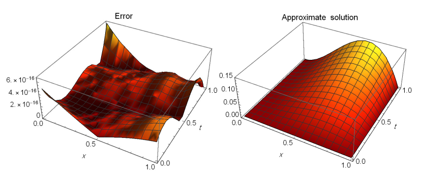
Additionally, Figure 1 illustrates the absolute errors (\(\mathcal{AE}\)) (left) and approximate solution (\(\mathcal{AS}\)) (right) for \(\alpha=0.75\) and \(\mathcal{N}=3\).
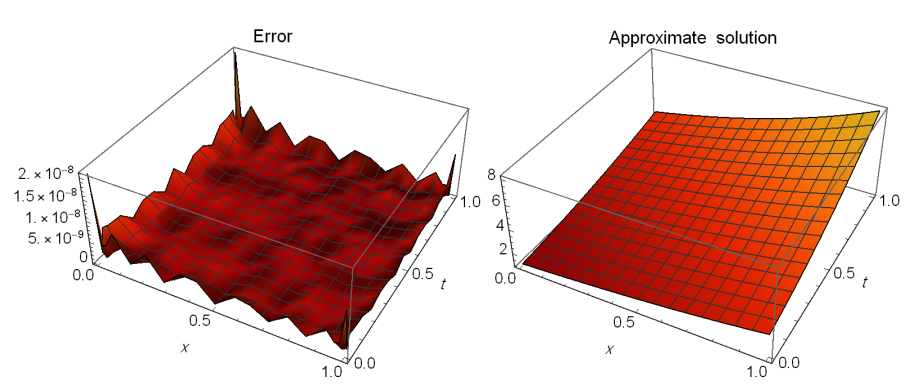
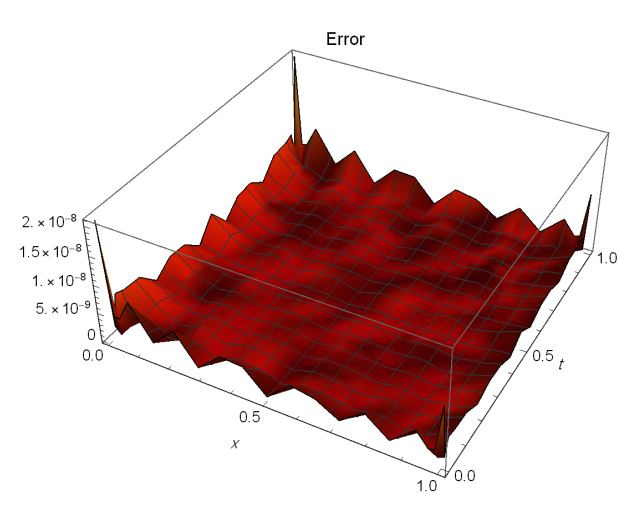
Problem 2. [39] Assuming \[{D_{t}^{\alpha}}\xi(z,t)-\mu\, \xi_{zz}(z,t)=t^3\, (z-1)\, z^4\,\frac{\Gamma (\alpha +4)}{6}-4\, z^2\, (5\, z-3)\, t^{\alpha +3}, \quad 0<\alpha\leq1, \tag{39}\] controlled by \[\xi(z,0)=e^z,\quad 0<z< 1, \tag{40}\] and \[\xi(0,t)=t^2+t+1,\quad \xi(1,t)=e \left(t^2+t+1\right), \quad 0<t< 1, \tag{41}\] where \(\xi(z,t)=\left(t^2+t+1\right) e^z\) is the analytic solution of this problem.
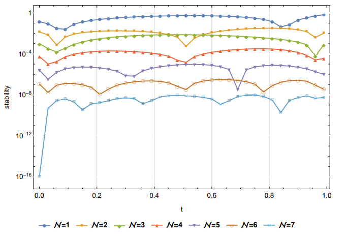
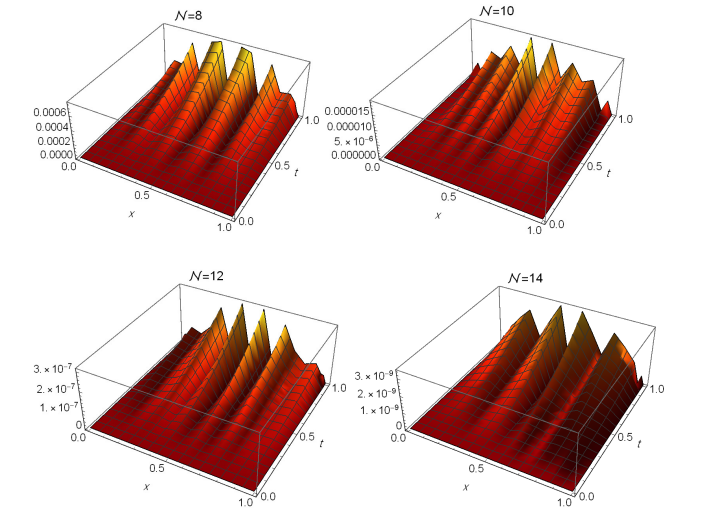
Table 1 compares the maximum \(\mathcal{AE}\) between our technique and that of [39] at various \(\alpha\) values when \(\mu=1\). Figure 2 illustrates the \(\mathcal{AE}\) (left) and \(\mathcal{AS}\) (right) for \(\alpha=0.75\) and \(\mathcal{N}=8\) when \(\mu=1\). Table 2 shows the \(\mathcal{AE}\) for \(\alpha=0.3\) and \(\mathcal{N}=8\) when \(\mu=1\). Figure 3 shows the \(\mathcal{AE}\) at \(\alpha=0.3\) and \(\mathcal{N}=8\) when \(\mu=2\). Finally, Figure 4 illustrates the stability \(|\xi^{\mathcal{N}+1}(z,t)-\xi^\mathcal{N}(z,t)|\) at \(z=t\) and different values of \(\mathcal{N}\) when \(\alpha=0.3\). These findings show that this method’s results are close to the exact solution.
| \(\alpha\) | Ref. [39] \((\mathcal{N}=64)\) | Proposed approach \((\mathcal{N} =8)\) |
|---|---|---|
| 0.25 | \(1.2889\times 10^{-5}\) | \(4.14712 \times 10^{-9}\) |
| 0.5 | \(1.1727\times 10^{-5}\) | \(2.07061 \times 10^{-9}\) |
| 0.75 | \(1.1645\times 10^{-5}\) | \(4.14649 \times 10^{-9}\) |
| \(z\) | \(t=0.2\) | \(t=0.5\) | \(t=0.8\) |
|---|---|---|---|
| 0.1 | \(9.92485\times 10^{-10}\) | \(1.28053\times 10^{-9}\) | \(1.01728\times 10^{-9}\) |
| 0.2 | \(1.3859\times 10^{-9}\) | \(1.79685\times 10^{-9}\) | \(1.49371\times 10^{-9}\) |
| 0.3 | \(1.26077\times 10^{-10}\) | \(1.67655\times 10^{-10}\) | \(1.48779\times 10^{-10}\) |
| 0.4 | \(1.17182\times 10^{-9}\) | \(1.52828\times 10^{-9}\) | \(1.32191\times 10^{-9}\) |
| 0.5 | \(5.85545\times 10^{-11}\) | \(7.65681\times 10^{-11}\) | \(5.56186\times 10^{-11}\) |
| 0.6 | \(1.05551\times 10^{-9}\) | \(1.37827\times 10^{-9}\) | \(1.20427\times 10^{-9}\) |
| 0.7 | \(1.91402\times 10^{-12}\) | \(2.99671\times 10^{-12}\) | \(2.37526\times 10^{-11}\) |
| 0.8 | \(9.63496\times 10^{-10}\) | \(1.25716\times 10^{-9}\) | \(1.07944\times 10^{-9}\) |
| 0.9 | \(6.59603\times 10^{-10}\) | \(8.53126\times 10^{-10}\) | \(6.84238\times 10^{-10}\) |
Problem 3. [38] Assuming \[{D_{t}^{\alpha}}\xi(z,t)-\xi_{zz}(z,t)= \left(4\,
\pi^2\, t^2+\frac{2\, t^{2-\alpha }}{\Gamma (3-\alpha )}\right)\,\sin
(2\, \pi\,z), \quad 0<\alpha\leq1, \tag{42}\] controlled by \[\xi(z,0)=0,\quad 0<z< 1, \tag{43}\] and \[\xi(0,t)=\xi(1,t)=0, \quad 0<t< 1, \tag{44}\]
where \(\xi(z,t)=t^{2}\,\sin(2\,\pi\,z)\)
constitutes the analytic solution to this problem.
Table 3 compares the maximum \(\mathcal{AE}\) between our technique and
that of [38] at
\(\alpha=0.5\). Figure 5 depicts the
maximum \(\mathcal{AE}\) at various
\(\mathcal{N}\) values for \(\alpha=0.5\). This image demonstrates the
advantage of adopting our strategy to obtain the maximum \(\mathcal{AE}\) for small values of \(\mathcal{N}.\) Table 4 shows the \(\mathcal{AE}\) at \(\alpha=0.9\) and \(\mathcal{N}=14\). It is clear that the
estimated and exact solutions are relatively close.
| Ref. [38] at \(\Delta t=0.001\) and \(M=64\) | Presented approach at \(\mathcal{N}=14\) |
|---|---|
| \(7.70\times 10^{-4}\) | \(8.03607 \times 10^{-10}\) |
| \(z\) | \(t=0.3\) | \(t=0.6\) | \(t=0.9\) |
|---|---|---|---|
| 0.1 | \(1.65467\times 10^{-9}\) | \(9.45648\times 10^{-10}\) | \(9.08267\times 10^{-11}\) |
| 0.2 | \(2.41125\times 10^{-9}\) | \(4.83308\times 10^{-10}\) | \(1.88788\times 10^{-9}\) |
| 0.3 | \(1.59463\times 10^{-9}\) | \(1.8858\times 10^{-9}\) | \(1.66441\times 10^{-9}\) |
| 0.4 | \(1.1292\times 10^{-9}\) | \(1.41938\times 10^{-10}\) | \(1.73461\times 10^{-9}\) |
| 0.5 | \(7.24165\times 10^{-11}\) | \(2.73845\times 10^{-10}\) | \(6.03381\times 10^{-10}\) |
| 0.6 | \(1.01843\times 10^{-9}\) | \(2.76671\times 10^{-10}\) | \(8.11171\times 10^{-10}\) |
| 0.7 | \(1.63854\times 10^{-9}\) | \(1.72031\times 10^{-9}\) | \(1.29951\times 10^{-9}\) |
| 0.8 | \(2.40511\times 10^{-9}\) | \(5.05605\times 10^{-10}\) | \(1.8508\times 10^{-9}\) |
| 0.9 | \(1.67916\times 10^{-9}\) | \(8.54546\times 10^{-10}\) | \(7.47452\times 10^{-11}\) |
This paper introduced an explicit Delannoy-tau spectral scheme for the numerical solution of the time-fractional diffusion equation with the Caputo derivative. By employing shifted Delannoy polynomials as basis functions, the method transforms the governing equation into a well-structured system of algebraic equations that can be solved without iterations. The proposed technique blends the precision of spectral approaches with the efficacy of explicit schemes, making it computationally attractive for large-scale or real-time simulations. Numerical examples confirm the precision and resilience of the approach. Future work may explore the application of the presented framework to multidimensional TFDEs, variable-order fractional models, and coupled systems arising in mathematical physics and engineering.