
The predator-prey relationships are the basis for the interaction of most species on planet Earth. This provides our complex ecosystems with rich biodiversity [1] and allows us to pertinently explain these systems using mathematical models. Using the coexistence conditions of prey and predators, renewable resources can be optimally managed [2]. Moreover, these systems can be used in physics, economics, chemical reactions, and many other fields to understand and explain natural phenomena. In the first half of the 20\(^{\text{th}}\) century, oscillations in prey and predator populations were captured by a model designed by Lotka [3] and Volterra [4]. This model was the starting point of a new way of designing mathematical models for competitive systems and generated a plethora of literature over time. To better capture the components of predator-prey interactions, various types of functional responses were proposed by Holling [5]. In [6], Leslie and Gower proposed that the carrying capacity of the predator’s environment should be proportional to the number of prey. The aim of this modification was to consider the physical phenomenon that the increase in the capacity of both predator and prey must be bounded. This phenomenon is not incorporated in the Lotka-Volterra model, but in [7] the Leslie-Gower model was proved to have a unique positive equilibrium as well as global asymptotic stability for any allowed parameters. Then, in [8], the stability with Holling functional responses was established. In [9], feedback controls were introduced, and the model was proved to be globally stable. Further properties of this model, like the Hopf bifurcation [10] and unique limit cycles [11], were proved. However, this model has its own drawbacks. One major drawback of this model arises in scenarios where the density of the prey population is low. In such cases, the predator cannot switch to alternative food sources [12].
This problem of alternative food sources is significant in natural settings, but it is not very important in some specific circumstances, such as harvesting. The exploitation of natural resources and other human activities has deeply perturbed the ecosystem on this planet. This perturbation is one of the major causes of global warming, which in turn contributes to changes in the migration patterns of different species or, in the worst cases, even their extinction. Harvesting of such species helps rectify such scenarios. Harvesting is also commonly practiced in fisheries, wildlife, and forestry management, showing the economically beneficial motivation of harvesting. Nevertheless, it has been observed that without scientific management, harvesting may bring more harm than good to nature. For example, in [13], the authors observed that more predator species are likely to become extinct if harvesting increases. Mesterton-Gibbons in [14] and Chaudhuri in [15] studied multi-species harvesting models. Kar et al. in [16] and Chaudhuri and Ray in [17] studied non-selective harvesting models of a prey-predator system in fisheries. In [18], the dynamics of predator-prey models with nonzero constant harvesting were studied, and in [19], the authors discussed constant proportion harvesting in a class of predator-prey models. Asfaw studied nonlinear harvesting in a time-dependent predator-prey model with non-autonomous dynamics in [20], whereas Leard et al. in [21] and Lenzini and Rebaza in [22] discussed the ratio-dependent model for harvesting. In [23], non-smooth threshold harvesting in a prey-predator model was considered, and the complex dynamics of the system were obtained.
Most of these models are designed using continuous derivatives. The benefits of continuous systems depend on the scenario in which they are used. Continuous systems explain those physical phenomena in which the target subject has overlapping time dynamics, such as the next generations or offspring. This is not true in all cases. There are many fish species, such as salmon, which spawn and are born at the same time each year. For such subjects of interest, discrete-time models are more suitable [24]. Discrete-time models are also used for studying organisms and species over time. They not only describe populations with non-overlapping generations better than their continuous counterparts but also elegantly show the chaotic behavior of nonlinear dynamics [25, 26]. However, this process of discretization is far from perfect. In fact, numerical oscillations are generally induced if classical finite difference schemes are used for the discretization of continuous systems, see [27, 28]. These methods use approximations to produce finite representations of functions, which is not sufficient if we want to probe into the dynamical behavior of the system. These methods produce fallacious numerical behavior, such as the creation of ghost equilibrium points, changes in the stability nature of existing equilibrium points, or destruction of domain invariance, revealing chaos, etc., which is not present in the actual model [29]. To rectify this aberration, the non-standard finite difference (NSFD) scheme was proposed by Mickens in [30]. He paved the way to construct discretization methods that deal with dynamical information, leading to a qualitative dynamical numerical scheme [29]. This method was named by Mickens as the Non-standard Finite Difference scheme.
A very special, complex, and interesting dynamic phenomenon also emerges in the investigation of bifurcations. This phenomenon is called chaos and has been studied for a long time. It focuses on the extreme sensitivity to initial conditions of the underlying dynamical laws of systems, which can even be deterministic in nature but, due to some hidden patterns, give highly irregular results with slight variations in the initial conditions. It has been shown to be present in most natural, physical, and social sciences as well as in mathematical biology. However, in most cases, it is not considered favorable, and over time, researchers have developed techniques to delay or even eliminate the chaotic behavior of systems. A state-feedback control with time delay was proposed by Chen and Yu in [31] for chaotic systems. The nonlinear state-feedback control was implemented by Abed et al. in [32] for controlling chaos introduced by period-doubling bifurcation. Luo et al. introduced a hybrid feedback control method in [33] to apply to period-doubling bifurcation, which was further shown to be applicable to Neimark-Sacker bifurcation as well. The OGY method was introduced by Ott et al. in [34], while Romeiras et al. proposed the pole-placement methodology in [35], which is also considered to be a generalization of the OGY method.
In this paper, we use the model proposed by Xie et al. in [36], in which they studied simultaneous harvesting for both prey and predator. They proved the boundedness, permanence, and stability of the model and discussed various bifurcations. They showed that under certain conditions, the model exhibits a stable limit cycle resulting from a supercritical Hopf bifurcation. In [36], they describe their model as \[\label{mainsys} \begin{cases} \dfrac{dx}{dt} = x\left(1 – x – \dfrac{\alpha y}{m + x} – \gamma\right),\\ \dfrac{dy}{dt} = y\left(\rho\left(1 – \dfrac{\beta y}{m + x}\right) – \delta\right), \end{cases} \tag{1}\] with the initial conditions: \(x(0) > 0\), \(y(0) > 0\). Here, \(x(t)\) and \(y(t)\) represent prey and predator densities, respectively, at time \(t\). All parameters in system (1) are positive.
In the remainder of this paper, we discretize system (1) by first applying the classical finite difference scheme in §2 and then create a non-standard finite difference scheme in §3, using the guidelines provided by Mickens in [30]. The topology and dynamics of the discrete system obtained using the classical finite difference method are given in §2.1 and §2.2; the existence of period-doubling bifurcation is given in §2.3, and the existence of Neimark-Sacker bifurcation is shown in §2.4. The corresponding numerical examples and graphs are given in §2.3.1 and §2.4.1, respectively. The same analysis for our non-standard finite difference scheme is presented in §3.1, §3.2, and §3.2.1, respectively. In §4, the chaos control techniques are presented. Finally, we conclude in §5.
There are different classical finite difference methods to discretize a continuous system. The ranking of these methods depends on their complexity and order. The most commonly used schemes are the Euler and Runge-Kutta methods, commonly known as integrator methods. In this work, we apply the forward Euler method to convert system (1) to its discrete counterpart. If we take \(k\) as the step size, then using the forward Euler method, (1) is given by \[\label{disc-sys} \begin{cases} x_{n+1} = x_n + k x_n\left(1 – x_n – \dfrac{\alpha y_n}{m + x_n} – \gamma\right), \\ y_{n+1} = y_n + k y_n \left(\rho \left(1 – \dfrac{\beta y_n}{m + x_n}\right) – \delta\right). \end{cases} \tag{2}\]
We solve the following system to find the fixed points of (2): \[\label{main-model} \begin{cases} x\left(1 – x – \dfrac{\alpha y}{m + x} – \gamma\right) = 0, \\ y\left(\rho\left(1 – \dfrac{\beta y}{m + x}\right) – \delta\right) = 0. \end{cases} \tag{3}\]
The system has three fixed points on the boundary, namely, \[\left\{E_1, E_2, E_3\right\} = \left\{\left(0,0\right), \left(0,\dfrac{m(\rho – \delta)}{\beta \rho}\right), \left(1 – \gamma, 0\right)\right\}.\]
For interior fixed points, we have the following cases:
i) If \(\delta > \rho\) or if \(\delta < \rho\) but \(\gamma > 1\), then there is no positive interior fixed point of the system.
ii) If \(\delta < \rho\) and \(\gamma < 1\), then there exists a unique positive interior fixed point of the system, namely, \[E_4 = \left(\bar{x}, \bar{y}\right) = \left(\dfrac{\alpha(\rho – \delta)}{\beta \rho} + 1 – \gamma, \dfrac{\rho – \delta}{\beta \rho}(m + \bar{x})\right).\]
The respective variational matrices at \(E_1\), \(E_2\), \(E_3\), and \(E_4\) are \[\begin{aligned} J_1 =& \left[ \begin{array}{cc} 1 + k\left(1 – \gamma\right) & 0 \\ 0 & 1 + k\left(\rho – \delta\right) \\ \end{array} \right],\\ J_2 =& \left[ \begin{array}{cc} 1 – k\left(1 – \gamma\right) & -k\dfrac{\alpha(1 – \gamma)}{1 – \gamma + m} \\ 0 & 1 + k\left(\rho – \delta\right) \\ \end{array} \right],\\ J_3 =& \left[ \begin{array}{cc} 1 + k\left(1 – \gamma – \dfrac{\alpha(\rho – \delta)}{\beta \rho}\right) & 0 \\ k\dfrac{(\rho – \delta)^2}{\beta \rho} & 1 – k\left(\rho – \delta\right) \\ \end{array} \right],\\ J_4 =& I + k\left[ \begin{array}{cc} A_1 & -A_2 \\ A_3 & -A_4 \\ \end{array} \right], \end{aligned}\] where \(A_1 = \bar{x}\left(\dfrac{\alpha \bar{y}}{(m + \bar{x})^2} – 1\right)\), \(A_2 = \dfrac{\alpha \bar{x}}{m + \bar{x}}\), \(A_3 = \dfrac{\beta \rho \bar{y}^2}{(m + \bar{x})^2}\), and \(A_4 = \rho – \delta\). To determine the stability of system (2) at each fixed point, we use the following lemma.
Lemma 1. Let \(t_i = \operatorname{Tr}(J_i)\), \(\det_i = \det(J_i)\), and \(p_i(z) = z^2 – t_i z + \det_i\), \(i = 1, \dots, 6\). Suppose \(z_1\), \(z_2\) are the roots of \(p(z)\). Then the fixed point is:
i) a sink, which is locally asymptotically stable if \(p(-1) > 0\) and \(\det < 1\).
ii) a source, which is locally unstable if \(p(-1) > 0\) and \(\det > 1\).
iii) a saddle if \(p(-1) < 0\).
iv) non-hyperbolic, and may exhibit a fold or transcritical bifurcation if \(p(1) = 0\).
v) non-hyperbolic, and may exhibit a period-doubling bifurcation if \(p(-1) = 0\) and \(t \neq -2, 0\).
vi) non-hyperbolic, and may exhibit a Neimark–Sacker bifurcation if \(4\det – t^2 > 0\) and \(\det = 1\).
Using Lemma 1, it is straightforward to show that \(E_1\) is always unstable, \(E_2\) is always a saddle, and \(E_3\) is stable if \(1 – \gamma < \dfrac{\alpha(\rho – \delta)}{\beta \rho}\) and a saddle if \(1 – \gamma > \dfrac{\alpha(\rho – \delta)}{\beta \rho}\). The stability analysis of the unique interior fixed point is richer and more central to our work.
Proposition 1. Let \(A_i\), \(i = 1, 2, 3, 4\) be as defined in §2.2, \[\label{eq:rho} \begin{cases} \rho_1 = \delta – A_1 + \dfrac{2\bar{y}}{m + \bar{x}}\left(\dfrac{A_2 \beta y}{m + \bar{x}} – \sqrt{A_2 \beta \left(\dfrac{A_2 \beta y^2}{(m + \bar{x})^2} + \delta – A_1\right)}\right), \\ \rho_2 = \delta – A_1 + \dfrac{2\bar{y}}{m + \bar{x}}\left(\dfrac{A_2 \beta y}{m + \bar{x}} + \sqrt{A_2 \beta \left(\dfrac{A_2 \beta y^2}{(m + \bar{x})^2} + \delta – A_1\right)}\right), \end{cases} \tag{4}\] and \[\label{eq:k} \begin{cases} k_1 = \dfrac{A_1 – A_4 – \sqrt{(A_1 + A_4)^2 – 4A_2A_3}}{A_1 A_4 – A_2 A_3}, \\ k_2 = \dfrac{A_1 – A_4 + \sqrt{(A_1 + A_4)^2 – 4A_2A_3}}{A_1 A_4 – A_2 A_3}. \end{cases} \tag{5}\]
For the positive interior fixed point \(E_4\), suppose \(\rho \notin \left(\rho_1, \rho_2\right)\). Then \(E_4\) is:
locally asymptotically stable if \(k \in \left(0, k_1\right)\);
locally unstable if \(k \in \left(k_2, \infty\right)\);
a saddle if \(k \in \left(k_1, k_2\right)\);
non-hyperbolic with eigenvalues \(z_1 = -1\) and \(\left\vert z_2\right\vert \neq 1\) if \(k = k_1\) or \(k = k_2\), and \(k \neq \dfrac{2}{A_4 – A_1}\) and \(k \neq \dfrac{4}{A_4 – A_1}\);
non-hyperbolic with complex conjugate eigenvalues, \(\left\vert z_1\right\vert = 1 = \left\vert z_2\right\vert\), if and only if \(k = \dfrac{A_1 – A_4}{A_1 A_4 – A_2 A_3}\) and \(k \in \left(0, \dfrac{4}{A_4 – A_1}\right)\).
Proof. Define \(p(z) = z^2 – t z + \det\) to be the characteristic polynomial of system (3) at \(E_4\), where \(t = 2 + (A_1 – A_4)k\) and \(\det = (A_2A_3 – A_1A_4)k^2 + (A_1 – A_4)k + 1\). For any \(k > 0\), \[p(-1) = (A_2A_3 – A_1A_4)k^2 + 2(A_1 – A_4)k + 4.\]
Thus, we can easily show that \[\begin{cases} p(-1) > 0, & \text{if } k \in \left(0, k_1\right) \cup \left(k_2, \infty\right), \\ p(-1) < 0, & \text{if } k \in \left(k_1, k_2\right), \\ p(-1) = 0, & \text{if } k = k_1 \text{ or } k = k_2. \end{cases}\]
Also, \[\begin{cases} \det > 1, & \text{if } k \in \left(\dfrac{A_1 – A_4}{A_1A_4 – A_2A_3}, \infty\right), \\ \det < 1, & \text{if } k \in \left(0, \dfrac{A_1 – A_4}{A_1A_4 – A_2A_3}\right), \\ \det = 1, & \text{if } k = \dfrac{A_1 – A_4}{A_1A_4 – A_2A_3}. \end{cases}\]
Then, using Lemma 1, we can state that \(E_4\) is:
a sink if and only if \[k \in \left\{\left(0, k_1\right) \cup \left(k_2, \infty\right)\right\} \cap \left(0, \dfrac{A_1 – A_4}{A_1A_4 – A_2A_3}\right) = \left(0, k_1\right);\]
a source if and only if \[k \in \left\{\left(0, k_1\right) \cup \left(k_2, \infty\right)\right\} \cap \left(\dfrac{A_1 – A_4}{A_1A_4 – A_2A_3}, \infty\right) = \left(k_2, \infty\right);\]
a saddle if and only if \(k \in \left(k_1, k_2\right)\);
non-hyperbolic with eigenvalues \(z_1 = -1\) and \(\left\vert z_2\right\vert \neq 1\) if and only if \(k = k_1\) or \(k = k_2\), and \(k \neq \dfrac{2}{A_4 – A_1}\) and \(k \neq \dfrac{4}{A_4 – A_1}\);
non-hyperbolic with \(z_{1,2} \in \mathbb{C}\) and \(\left\vert z_1\right\vert = 1 = \left\vert z_2\right\vert\) if and only if \(k = \dfrac{A_1 – A_4}{A_1 A_4 – A_2 A_3}\) and \(k \in \left(0, \dfrac{4}{A_4 – A_1}\right)\).
◻
Define, \[\begin{aligned} \Omega_{PD} &=& \left\{\left(\alpha, \beta, \delta, m, \gamma, \rho, k_0\right) \in \mathbb{R}^7_+ : k_0 = k_1 \text{ or } k_2,\hspace{2mm} k_0 \neq \dfrac{2}{A_4 – A_1}, k_0 \neq \dfrac{4}{A_4 – A_1}, \hspace{2mm} \rho \notin \left(\rho_1, \rho_2\right) \right\}. \end{aligned}\]
Let \(\left(\alpha, \beta, \delta, m, \gamma, \rho, k\right) \in \Omega_{PD}\), \(k\) be the bifurcation parameter. To perturb \(k\), let \(K\) be such that \(\left\vert K\right\vert \lll 1\). The perturbed mapping is, \[\left( \begin{array}{c} x \\ y \\ \end{array} \right) \to \left( \begin{array}{c} x + \left(k + K\right) x\left(1 – x – \dfrac{\alpha y}{m + x} – \gamma\right) \\ y + \left(k + K\right)y\left(\rho \left(1 – \dfrac{\beta y}{m + x}\right) – \delta\right) \\ \end{array} \right).\]
In order to translate the fixed point to \(\left(0, 0\right)\), assume \(x = X + \bar{x}\) and \(y = Y + \bar{y}\). Then with the help of Taylor series expansion, the above mapping can be written as: \[\label{mod-sys-PD-FD} \left( \begin{array}{c} X \\ Y \\ \end{array} \right) \to \left( \begin{array}{cc} a_{11} & a_{12} \\ a_{21} & a_{22} \\ \end{array} \right) \left( \begin{array}{c} X \\ Y \\ \end{array} \right) + \left( \begin{array}{c} f_{PD}\left(X, Y, K\right) \\ g_{PD}\left(X, Y, K\right) \\ \end{array} \right), \tag{6}\] where \(a_{11} = 1 + k A_1\), \(a_{12} = -k A_2\), \(a_{21} = k A_3\), \(a_{22} = 1 – k A_4\), \(f_{PD}\left(X, Y, K\right) = k b_1 X^2 + k b_2 X Y + A_1 K X – A_2 K Y + k b_3 Y^2 + k b_4 X^3 + k b_5 X^2 Y + b_1 K X^2 + b_2 K X Y + b_3 K Y^2 + k b_6 X Y^2 + k b_7 Y^3 + O\left(\left\vert X + Y + K\right\vert^4\right)\) and \(g_{PD}\left(X, Y, K\right) = k b_8 X^2 + k b_9 X Y + A_3 K X – A_4 K Y + k b_{10} Y^2 + k b_{11} X^3 + k b_{12} X^2 Y + b_8 K X^2 + b_9 K X Y + b_{10} K Y^2 + k b_{13} X Y^2 + k b_{14} Y^3 + O\left(\left\vert X + Y + K\right\vert^4\right)\), where, \(b_1 = \dfrac{\alpha m \bar{y}}{(m+\bar{x})^3} – 1\), \(b_2 = – \dfrac{\alpha m}{(m+\bar{x})^2}\), \(b_3 = 0\), \(b_4 = -\dfrac{\alpha m \bar{y}}{(m+\bar{x})^4}\), \(b_5 = \dfrac{\alpha m}{(m+\bar{x})^3}\), \(b_6 = 0\), \(b_7 = 0\), \(b_8 = -\dfrac{\rho \beta \bar{y}^2}{(m+\bar{x})^3}\), \(b_9 = \dfrac{2 \rho \beta \bar{y}}{m+\bar{x}}\), \(b_{10} = -\dfrac{\beta \rho }{m+\bar{x}}\), \(b_{11} = \dfrac{\rho \beta \bar{y}^2}{(m+\bar{x})^4}\), \(b_{12} = -\dfrac{2 \rho \beta \bar{y} }{(m+\bar{x})^3}\), \(b_{13} = \dfrac{\beta \rho }{(m+\bar{x})^2}\) and \(b_{14} = 0\).
To convert the system (6) into the normal form of period-doubling bifurcation, let \[\begin{aligned} \label{eq:SFD-PD-1} \left( \begin{array}{c} X \\ Y \\ \end{array} \right) &=& T_{PD}\left( \begin{array}{c} u \\ v \\ \end{array} \right) = \left( \begin{array}{cc} a_{12} & a_{12} \\ -1 – a_{11} & z_2 – a_{22} \\ \end{array} \right)\left( \begin{array}{c} u \\ v \\ \end{array} \right), \end{aligned} \tag{7}\] where \(T_{PD}\) is an invertible matrix. If we define \[\begin{aligned} d_1 =& c_1 k \left(a_{12} \left(a_{11}+1\right) \left(b_9-b_2 c_2\right)+a_{12}^2 \left(b_1 c_2-b_8\right)+\left(a_{11}+1\right){}^2 \left(-b_{10}\right)\right), \\ d_2 =& c_1 (-k) \left(-a_{12} \left(a_{11}+a_{22}-z_2+1\right) \left(b_9-b_2 c_2\right)+2 a_{12}^2 \left(b_8-b_1 c_2\right)+ 2 \left(a_{11}+1\right) b_{10} \left(a_{22}-z_2\right)\right), \\ d_3 =& c_1 \left(a_{12} \left(A_1 c_2+A_3\right)+\left(a_{11}+1\right) \left(A_2 c_2-A_4\right)\right), \\ d_4 =& c_1 \left(\left(a_{22}-z_2\right) \left(A_2 c_2-A_4\right)+a_{12} \left(A_1 c_2+A_3\right)\right), \\ d_5 =& c_1 k \left(a_{12} \left(a_{22}-z_2\right) \left(b_9-b_2 c_2\right)+a_{12}^2 \left(b_1 c_2-b_8\right)-b_{10} \left(a_{22}-z_2\right){}^2\right), \\ d_6 =& c_1 k \left(a_{12}^3 \left(b_4 c_2-b_{11}\right)+\left(a_{11}+1\right) a_{12}^2 \left(b_{12}-b_5 c_2\right)-\left(a_{11}+1\right){}^2 a_{12} b_{13}\right), \\ d_7 =& c_1 k \left(a_{12}^2 \left(2 a_{11}+a_{22}-z_2+2\right) \left(b_{12}-b_5 c_2\right)-3 a_{12}^3 \left(b_{11}-b_4 c_2\right)- \left(a_{11}+1\right) a_{12} b_{13} \left(a_{11}+2 a_{22}-2 z_2+1\right)\right), \\ d_8 =& c_1 \left(a_{12} \left(a_{11}+1\right) \left(b_9-b_2 c_2\right)+a_{12}^2 \left(b_1 c_2-b_8\right)+\left(a_{11}+1\right){}^2 \left(-b_{10}\right)\right), \\ d_9 =& -c_1 \left(-a_{12} \left(a_{11}+a_{22}-z_2+1\right) \left(b_9-b_2 c_2\right)+2 a_{12}^2 \left(b_8-b_1 c_2\right)+ 2 \left(a_{11}+1\right) b_{10} \left(a_{22}-z_2\right)\right), \\ d_{10} =& c_1 \left(a_{12} \left(a_{22}-z_2\right) \left(b_9-b_2 c_2\right)+a_{12}^2 \left(b_1 c_2-b_8\right)-b_{10} \left(a_{22}-z_2\right){}^2\right), \\ d_{11} =& c_1 k \left(a_{12}^2 \left(a_{11}+2 a_{22}-2 z_2+1\right) \left(b_{12}-b_5 c_2\right)-3 a_{12}^3 \left(b_{11}-b_4 c_2\right)- a_{12} b_{13} \left(a_{22}-z_2\right) \left(2 a_{11}+a_{22}-z_2+2\right)\right),\\ d_{12} =& c_1 k \left(a_{12}^2 \left(a_{22}-z_2\right) \left(b_{12}-b_5 c_2\right)+a_{12}^3 \left(b_4 c_2-b_{11}\right)-a_{12} b_{13} \left(a_{22}-z_2\right){}^2\right), \\ d_{13} =& c_1 k \left(a_{12} \left(a_{11}+1\right) \left(-b_2 c_3-b_9\right)+a_{12}^2 \left(b_1 c_3+b_8\right)+\left(a_{11}+1\right){}^2 b_{10}\right), \\ d_{14} =& c_1 (-k) \left(a_{12} \left(a_{11}+a_{22}-z_2+1\right) \left(b_2 c_3+b_9\right)-2 a_{12}^2 \left(b_1 c_3+b_8\right)- 2 \left(a_{11}+1\right) b_{10} \left(a_{22}-z_2\right)\right), \\ d_{15} =& c_1 \left(a_{12} \left(A_1 c_3+A_3\right)+\left(a_{11}+1\right) \left(A_2 c_3-A_4\right)\right), \\ d_{16} =& c_1 \left(\left(a_{22}-z_2\right) \left(A_2 c_3-A_4\right)+a_{12} \left(A_1 c_3+A_3\right)\right),\\ d_{17} =& c_1 k \left(-a_{12} \left(a_{22}-z_2\right) \left(b_2 c_3+b_9\right)+a_{12}^2 \left(b_1 c_3+b_8\right)+b_{10} \left(a_{22}-z_2\right){}^2\right), \\ d_{18} =& c_1 k \left(a_{12}^3 \left(b_4 c_3+b_{11}\right)-\left(a_{11}+1\right) a_{12}^2 \left(b_5 c_3+b_{12}\right)+\left(a_{11}+1\right){}^2 a_{12} b_{13}\right), \\ d_{19} =& c_1 k \left(-a_{12}^2 \left(2 a_{11}+a_{22}-z_2+2\right) \left(b_5 c_3+b_{12}\right)+3 a_{12}^3 \left(b_4 c_3+b_{11}\right)+ \left(a_{11}+1\right) a_{12} b_{13} \left(a_{11}+2 a_{22}-2 z_2+1\right)\right), \\ d_{20} =& c_1 \left(-a_{12} \left(a_{11}+1\right) \left(b_2 c_3+b_9\right)+a_{12}^2 \left(b_1 c_3+b_8\right)+\left(a_{11}+1\right){}^2 b_{10}\right), \\ d_{21} =& -c_1 \left(a_{12} \left(a_{11}+a_{22}-z_2+1\right) \left(b_2 c_3+b_9\right)-2 a_{12}^2 \left(b_1 c_3+b_8\right)- 2 \left(a_{11}+1\right) b_{10} \left(a_{22}-z_2\right)\right), \\ d_{22} =& c_1 \left(-a_{12} \left(a_{22}-z_2\right) \left(b_2 c_3+b_9\right)+a_{12}^2 \left(b_1 c_3+b_8\right)+b_{10} \left(a_{22}-z_2\right){}^2\right), \\ d_{23} =& c_1 k \left(-a_{12}^2 \left(a_{11}+2 a_{22}-2 z_2+1\right) \left(b_5 c_3+b_{12}\right)+3 a_{12}^3 \left(b_4 c_3+b_{11}\right)+ a_{12} b_{13} \left(a_{22}-z_2\right) \left(2 a_{11}+a_{22}-z_2+2\right)\right), \\ d_{24} =& c_1 k \left(-a_{12}^2 \left(a_{22}-z_2\right) \left(b_5 c_3+b_{12}\right)+a_{12}^3 \left(b_4 c_3+b_{11}\right)+a_{12} b_{13} \left(a_{22}-z_2\right){}^2\right) ,\\ X =& a_{12}\left(u + v\right),\\ Y =& -(1 + a_{11}) u + (z_2 – a_{22}) v, \end{aligned}\] and \[\begin{aligned} \tilde{f}_{PD}\left(u, v, K\right) =&d_1 u^2 + d_2 u v + d_3 K u + d_4 K v + d_5 v^2 + d_6 u^3 + d_7 u^2 v + d_8 K u^2 + d_9 K u v + d_{10} K v^2 + d_{11} u v^2 + d_{12} v^3 \\ & + O\left(\left\vert u + v + K\right\vert^4\right) ,\\ \tilde{g}_{PD}\left(u, v, K\right) =& d_{13} u^2 + d_{14} u v + d_{15} K u + d_{16} K v + d_{17} v^2 + d_{18} u^3 + d_{19} u^2 v + d_{20} K u^2 + d_{21} K u v + d_{22} K v^2 + d_{23} u v^2 \\ &+ d_{24} v^3 + O\left(\left\vert u + v + K\right\vert^4\right), \end{aligned}\] then (7) can be written as \[\begin{aligned} \label{finalsys} \left( \begin{array}{c} u \nonumber \\ v \nonumber \\ \end{array} \right) \to& \left( \begin{array}{cc} -1 & 0 \\ 0 & z_2 \\ \end{array} \right) \left( \begin{array}{c} u \\ v \\ \end{array} \right) + \left( \begin{array}{c} \tilde{f}_{PD}\left(u, v, K\right) \nonumber \\ \tilde{g}_{PD}\left(u, v, K\right) \nonumber \\ \end{array} \right) . \end{aligned}\]
In order to convert to normal form, let \(M_{C}\left(0, 0, 0\right)\) be the center manifold of (8), evaluated at \((0, 0)\) in a small neighborhood of \(K = 0\). Let \[\begin{aligned} M_{C} = \left\{\left(K, u, v\right) : v = G_{PD}\left(K, u\right), \left\vert u\right\vert < \delta_{1}, \left\vert K\right\vert < \delta_{2}, G_{PD}(0, 0) = 0, DG_{PD}(0,0) = 0 \right\}, \end{aligned}\] and \[G_{PD}\left(K, u\right) = m_1 u^2 + m_2 K u + m_3 K^2 + O\left(\left\vert K + u\right\vert^3\right).\]
Define, \[\begin{aligned} F_{PD} \left(K, G_{PD}\left(K, u\right)\right) = G_{PD}\left(K, – u + \tilde{f}_{PD}\left(K, u, G_{PD}\left(K, u\right)\right)\right) – z_2 G_{PD}\left(K, u\right) – \tilde{g}_{PD}\left(K, u, G_{PD}\left(K, u\right)\right). \end{aligned}\]
By comparing coefficients in the equation \(F_{PD} \left(K, G_{PD}\left(K, u\right)\right) = 0\), we get, \[m_1 = \dfrac{d_{13}}{1-z_2}, \hspace{3mm} m_2 = -\dfrac{d_{15}}{1+z_2}, \hspace{3mm} m_3 = 0.\]
Thus, by center manifold theorem, the following map gives dynamics restricted to \(M_{C}\): \[\begin{aligned} F_C \hspace{3mm} : \hspace{3mm} u &\mapsto& – u + d_1 u^2 + d_3 K u – \dfrac{d_4 d_{15}}{1 + z_2} K^2 u + \left(d_8 – \dfrac{d_4 d_{13}}{1 – z_2} – \dfrac{d_2 d_{15}}{1 + z_2}\right) K u^2 \\ && + \left(d_6 + \dfrac{d_2 d_{13}}{1 – z_2}\right) u^3 + O\left(\left\vert K + u\right\vert^4\right). \end{aligned}\]
Furthermore, define \[\begin{aligned} \Upsilon_1 &=& \left(\dfrac{\partial^2 F_C}{\partial K \partial u} + \dfrac{1}{2}\dfrac{\partial F_C}{\partial K}\dfrac{\partial^2 F_C}{\partial u^2}\right)_{\left(0, 0\right)} = d_3 \neq 0, \\ \Upsilon_2 &=& \left(\dfrac{1}{6}\dfrac{\partial^3 F_C}{\partial u^3} + \left(\dfrac{1}{2}\dfrac{\partial^2 F_C}{\partial u^2}\right)^2\right)_{\left(0, 0\right)} = d_1^2 + d_6 + \dfrac{d_2 d_{13}}{1-z_2} \neq 0. \end{aligned}\]
Theorem 1. If \(\Upsilon_1 \neq 0\) and \(\Upsilon_2 \neq 0\), then if \(k\) varies in small neighborhood of \(k_1\) or \(k_2\) then the system (2) exhibits period-doubling bifurcation at the interior fixed point when parameter. Moreover, the period-two orbits that bifurcate from the interior fixed point are unstable if \(\Upsilon_2 < 0\) and stable if \(\Upsilon_2 > 0\).
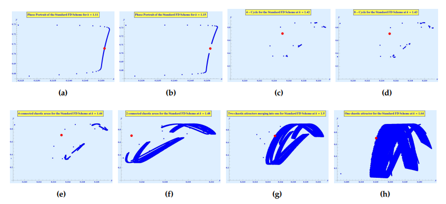
Select \(\left(\alpha, \beta, \delta, m, \gamma, \rho, k_0\right)\) \(=\) \(\left(0.07, 1.9, 0.1, 1.2, 0.75, 1.9, 1.11\right)\), \(k \in [1, 1.4]\) and the initial value \((x_0, y_0) = (0.45, 0.5)\). The fixed point is \(\left(\bar{x}, \bar{y}\right)\) \(=\) \(\left(0.215097,0.705589\right)\). The Jacobian matrix at \(\left(\bar{x}, \bar{y}\right)\) is \[\left( \begin{array}{cc} 1 – 0.209792 k & -0.0106401 k \\ 0.897507 k & 1 – 1.8 k \\ \end{array} \right),\] with eigenvalues \(z_1 = -1\) and \(z_2 = 0.759395\). For any positive \(k\), the eigenvalues are less then \(1\) and \(z_2 = -1\), if \(k \neq 1.11484\), or, \(k \neq 9.26699\). Thus, the fixed point is stable for any \(k \neq 1.11484\), or, \(k \neq 9.26699\), otherwise, the fixed point undergoes period-doubling bifurcation, as \(k\) varies in the small neighborhood of \(k_0\), where we let \(k_0 = 1.11484\). After calculations, we get, \(\Upsilon_1 = 0.00602808 \neq 0\) and \(\Upsilon_2 = 57.4343 \neq 0\). These values proves the correctness of Theorem 1 and rectify the dynamics of system (2) observed in §2.3. Moreover, \(\Upsilon_2 > 0\), which shows that the stability of period-two orbits that bifurcate from positive equilibrium.
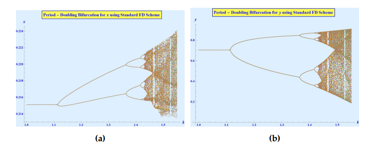
It is apparent from Figure 1a that the fixed point \(\left(0.215097,0.705589\right)\) of system (2) is stable for \(k < 1.11484\) and it becomes unstable due to period doubling bifurcation around \(1.11484\), see Figure 1b. In Figure 1c, we get a stable period \(4\)-cycle, which in bifurcation diagram, Figure 2, can easily be seen around \(k = 1.42\). As the value of the bifurcation parameter \(k\) is slightly increased, the dynamics of the system exhibits a stable period \(8\)-cycle around \(k = 1.43\). This can also easily be seen in the bifurcation diagrams in Figure 2.
If we further increase the parameter \(k\) to \(1.44\), the increment gives rise to a dynamic of four connected attractors, as can be seen in Figure 1e. Further increment in \(k\) to \(1.48\) gives rise to a dynamic of two connected attractors, Figure 1f, which then finally evolves into a one-piece chaotic attractor, see Figures 1g and 1h.
Define, \[\begin{aligned} \Omega_{NS} =& \left\{\left(\alpha, \beta, \delta, m, \gamma, \rho, k_0\right) \in \mathbb{R}^7_+ : k_0 = \dfrac{A_1 – A_4}{A_1 A_4 – A_2 A_3}, \hspace{2mm} k \in \left(0, \dfrac{4}{A_4 – A_1}\right) \right\}. \end{aligned}\]
Let \(\left(\alpha, \beta, \delta, m, \gamma, \rho, k\right) \in \Omega_{NS}\), i-e, \(k=\dfrac{A_1-A_4}{A_1 A_4-A_2 A_3}\). Let \(K\) be as defined before. Then the perturbed mapping is given by \[\left( \begin{array}{c} x \\ y \\ \end{array} \right) \to \left( \begin{array}{c} x + \left(k + K\right) x\left(1 – x – \dfrac{\alpha y}{m + x} – \gamma\right) \\ y + \left(k + K\right)y\left(\rho \left(1 – \dfrac{\beta y}{m + x}\right) – \delta\right) \\ \end{array} \right).\]
In order to translate the fixed point to \(\left(0, 0\right)\), assume \(x = X + \bar{x}\) and \(y = Y + \bar{y}\). Then with the help of Taylor series expansion, the above mapping can be written as \[\label{mod-sys-NS-FD} \left( \begin{array}{c} X \\ Y \\ \end{array} \right) \to \left( \begin{array}{cc} c_{11} & c_{12} \\ c_{21} & c_{22} \\ \end{array} \right) \left( \begin{array}{c} X \\ Y \\ \end{array} \right) + \left( \begin{array}{c} f_{NS}\left(X, Y\right) \\ g_{NS}\left(X, Y\right) \\ \end{array} \right), \tag{8}\] where \(c_{11} = 1 + \left(k+K\right)A_1\), \(c_{12} = -\left(k+K\right)A_2\), \(c_{21} = \left(k+K\right)A_3\), \(c_{22} = 1 – \left(k+K\right)A_4\), and \[\begin{aligned} % \nonumber % Remove numbering (before each equation) f_{NS}\left(X, Y\right) =& \left(k+K\right)b_1 X^2 + \left(k+K\right)b_2 X Y + \left(k+K\right) b_3 Y^2 + k b_4 X^3 + k b_5 X^2 Y + k b_6 X Y^2 + k b_7 Y^3\\& + O\left(\left\vert X + Y\right\vert^4\right), \\ g_{NS}\left(X, Y\right) =& \left(k+K\right) b_8 X^2 + \left(k+K\right) b_9 X Y + \left(k+K\right)b_{10} Y^2 + k b_{11} X^3 + k b_{12} X^2 Y + k b_{13} X Y^2 + k b_{14} Y^3 \\&+ O\left(\left\vert X + Y\right\vert^4\right), \end{aligned}\] and \(b_i, \hspace{2mm} i \in \left\{1, 2, \ldots, 14\right\}\) be the same as defined in §2.3. Let \(p_{NS}(z)\) be the characteristic polynomial of the variational matrix in (8) defined as \[\label{ch-pol-NS} p_{NS}(z) = z^2 – P(K) z + Q(K), \tag{9}\] where \(P(K) = c_{11} + c_{22}\) and \(Q(K) = c_{11} c_{22} – c_{21}c_{12}\). Since \(\left(\alpha, \beta, \delta, m, \gamma, \rho, k\right) \in \Omega_{NS}\), the eigenvalues \(z_1\) and \(z_2\) are complex conjugate with \(\left\vert z_1\right\vert = \left\vert z_2\right\vert = 1\). This also shows that \(z_{1,2} = \dfrac{P(K)}{2} \pm \dfrac{\iota}{2} \sqrt{4 Q(K) – P(K)^2}\) and \(1 = \left\vert z_1\right\vert = \left\vert z_2\right\vert = \sqrt{Q(K)}\). Note that \(P(K)^2 -4 Q(K) < 0\), which implies that \(P(K)^2 < 4Q(K)\) or \(P(K) \in \left(-2,2\right)\). Also, if \(\rho \neq \delta + \bar{x} \left(\dfrac{\alpha \bar{y}}{\left(\bar{x}+m\right)^2}-1\right)\), then \[\left(\dfrac{d\left|z_{1, 2}\right|}{d K}\right)_{K=0} = \dfrac{1}{2} \left(\rho – \delta – \bar{x} \left(\dfrac{\alpha \bar{y}}{(m+\bar{x})^2}-1\right)\right) \neq 0.\]
To check whether the unit circle of coordinate axis do not contains the roots of (9) at \(K = 0\) at the intersection, we need to ensure that \(z_{1,2}^m \neq 1\) for \(m = 1, 2, 3, 4\). It will be true if we can show that \(P(0) \neq -2, 0, 1, 2\). Since, \(\left(\alpha, \beta, \delta, m, \gamma, \rho, k\right) \in \Omega_{NS}\), we already know that \(P(0) \neq -2, 0, 2\). Finally, \(P(0) \neq 1\) if and only if \(k \neq \dfrac{1}{A_4-A_1}\). Now, to convert system (8) to the normal form at \(K = 0\), define \[T_{NS} = \left( \begin{array}{cc} 0 & 1 \\ S & R \\ \end{array} \right),\] where \(R=\dfrac{P(0)}{2}\) and \(S = \dfrac{1}{2} \sqrt{4Q(0) – P(0)^2}\). Here, \(T_{NS}\) is an invertible matrix. If we consider the transformation \[\left( \begin{array}{c} X \\ Y \\ \end{array} \right)=T_{NS} \left( \begin{array}{c} u \\ v \\ \end{array} \right),\] and define \[\begin{aligned} e_1 =& \dfrac{(k+K) \left(-R \left(b_2 S+b_1\right)+S \left(b_{10} S+b_9\right)+b_8\right)}{S}, \\ e_2 =& \dfrac{\left(b_2 (-R)+2 b_{10} S+b_9\right) (R (k+K))}{S}, \\ e_3 =& \dfrac{b_{10} \left(R^2 (k+K)\right)}{S}, \\ e_4 =& \dfrac{k \left(-R \left(b_5 S+b_4\right)+S \left(b_{13} S+b_{12}\right)+b_{11}\right)}{S}, \\ e_5 =& \dfrac{(k R) \left(\left(2 b_{13} S+b_{12}\right)-b_5 R\right)}{S} \\ e_6 =& \dfrac{b_{13} \left(k R^2\right)}{S}, \\ e_7 =& 0, \\ e_8 =& \left(b_2 S+b_1\right) (k+K),\\ e_9 =& b_2 R (k+K), \\ e_{10} =& 0, \\ e_{11} =& k \left(b_5 S+b_4\right),\\ e_{12} =& b_5 k R, \\ e_{13} =& 0, \\ e_{14} =& 0, \\ X =& v, \\ Y =& S u + R v, \end{aligned}\] and \[\begin{aligned} \tilde{f}_{NS}\left(u, v\right) =& e_1 u^2 + e_2 u v + e_3 v^2 + e_4 u^3 + e_5 u^2v + e_6 u v^2 + e_7 v^3 + O\left(\left\vert u + v\right\vert^4\right) ,\\ \tilde{g}_{NS}\left(u, v\right) =& e_8 u^2 + e_8 u v + e_{10} v^2 + e_{11} u^3 + e_{12} u^2 v + e_{13} u v^2 + e_{14} v^3 + O\left(\left\vert u + v\right\vert^4\right). \end{aligned}\]
System (8) is thus transformed into \[\begin{aligned} \label{mod-sys-NS} \left( \begin{array}{c} u \\ v \\ \end{array} \right) \to& \left( \begin{array}{cc} R & -S \\ S & R \\ \end{array} \right) \left( \begin{array}{c} u \\ v \\ \end{array} \right) + \left( \begin{array}{c} \tilde{f}_{NS}\left(u, v\right) \\ \tilde{g}_{NS}\left(u, v\right) \\ \end{array} \right). \end{aligned} \tag{10}\]
In order for the map (10) to exhibit Neimark-Sacker bifurcation, the following quantity must be non-zero: \[\label{quantity-NS} M_{NS} = \left( \biggl[-\operatorname{Re} \left(\varpi_{20}\varpi_{11}\dfrac{\left(1 – 2z_{1}\right)z_{2}^{2}}{1 – z_{1}}\right) – \dfrac{1}{2} \left\vert\varpi_{11}\right\vert^{2} – \left\vert\varpi _{02}\right\vert^{2} + \operatorname{Re}(\varpi_{21}z_{2}) \biggr]\right)_{K=0}, \tag{11}\] where \[\begin{aligned} % \nonumber % Remove numbering (before each equation) \varpi_{20} =& \dfrac{1}{8} \left[ \dfrac{\partial^2 \bar{f}_{NS}}{\partial u^2} – \dfrac{\partial^2 \bar{f}_{NS}}{\partial v^2} + 2\dfrac{\partial^2 \bar{g}_{NS}}{\partial u \partial v} + \iota \left(\dfrac{\partial^2 \bar{g}_{NS}}{\partial u^2} – \dfrac{\partial^2 \bar{g}_{NS}}{\partial v^2} – 2\dfrac{\partial^2 \bar{f}_{NS}}{\partial u \partial v}\right) \right], \\ \varpi_{11} =& \dfrac{1}{4} \left[ \dfrac{\partial^2 \bar{f}_{NS}}{\partial u^2} + \dfrac{\partial^2 \bar{f}_{NS}}{\partial v^2} + \iota \left(\dfrac{\partial^2 \bar{g}_{NS}}{\partial u^2} + \dfrac{\partial^2 \bar{f}_{NS}}{\partial v^2}\right) \right] ,\\ \varpi_{02} =& \dfrac{1}{8} \left[ \dfrac{\partial^2 \bar{f}_{NS}}{\partial u^2} – \dfrac{\partial^2 \bar{f}_{NS}}{\partial v^2} – 2\dfrac{\partial^2 \bar{g}_{NS}}{\partial u \partial v} + \iota \left(\dfrac{\partial^2 \bar{g}_{NS}}{\partial u^2} – \dfrac{\partial^2 \bar{g}_{NS}}{\partial v^2} + 2\dfrac{\partial^2 \bar{f}_{NS}}{\partial u \partial v}\right) \right] ,\\ \varpi_{21} =& \dfrac{1}{16} \left[\dfrac{\partial^3 \bar{f}_{NS}}{\partial u^3} + \dfrac{\partial^3 \bar{f}_{NS}}{\partial u \partial v^2} + \dfrac{\partial^3 \bar{g}_{NS}}{\partial u^2 \partial v} + \dfrac{\partial^3 \bar{g}_{NS}}{\partial v^3}+ \iota \left(\dfrac{\partial^3 \bar{g}_{NS}}{\partial u^3} + \dfrac{\partial^3 \bar{g}_{NS}}{\partial u \partial v^2} – \dfrac{\partial^3 \bar{f}_{NS}}{\partial u^2 \partial v} – \dfrac{\partial^3 \bar{f}_{NS}}{\partial v^3}\right) \right]. \end{aligned}\]
Using the theorem in [37], we have the following result.
Theorem 2. If \(k \neq \dfrac{1}{A_4-A_1}\), \(M_{NS}\) defined in (11) is non-zero, \(\left(\alpha, \beta, \delta, m, \gamma, \rho, k\right) \in \Omega_{NS}\) and \(k\) varies \(k_0 = \dfrac{A_1-A_4}{A_1 A_4-A_2 A_3}\), then system (3) exhibits Neimark-Sacker bifurcation at the unique fixed point \(\left(\bar{x}, \bar{y}\right)\). Moreover, a repelling invariant closed curve bifurcate from the fixed point \(\left(\bar{x}, \bar{y}\right)\) for \(k < k_0\), if \(M_{NS} > 0\). Similarly, an attracting invariant closed curve bifurcate from the fixed point for \(k > k_0\), if \(M_{NS} < 0\).
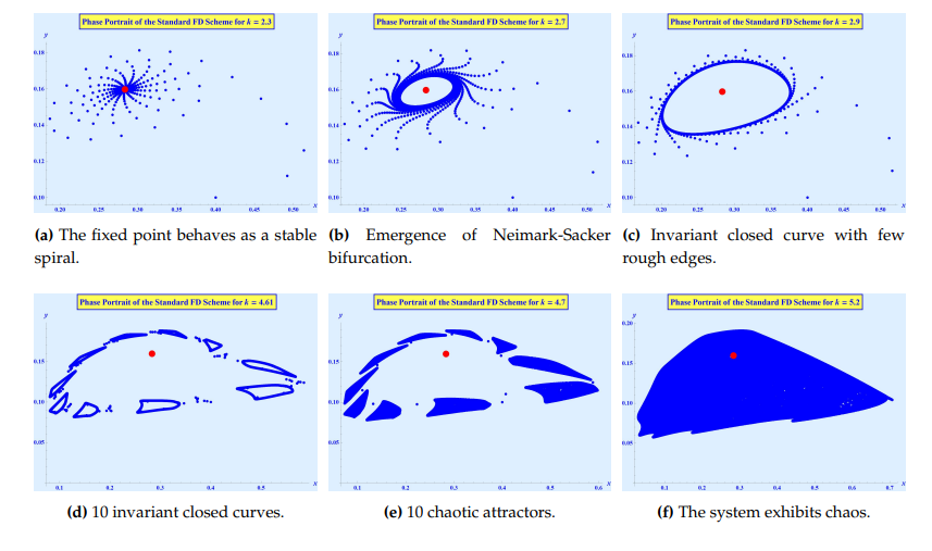
Take, \(\left(\alpha, \beta, \delta, m, \gamma, \rho\right)\) \(=\) \(\left(1, 0.6, 0.3, 0.1, 0.3, 0.4\right)\), \(k \in [2.2,5.2]\) and the initial value \((x_0, y_0) = \left(0.4, 0.1\right)\). For \(k = k_0 = 2.65985\), the Jacobian matrix is \[\left( \begin{array}{cc} 1 + 0.0246377 k & -0.73913 k \\ 0.0416667 k & 1 – 0.1 k \\ \end{array} \right),\] with \(z_1 = 0.899774 – 0.436356\iota\) and \(z_2 = 0.899774 + 0.436356\iota\) being the eigenvalues. Both eigenvalues lie on the unit circle. Also, \(k_0 \neq \dfrac{1}{A_4-A_1} = 13.2692\), \(k_0 \in \left(0, \dfrac{4}{A_4 – A_1}\right) = \left(0, 53.0769\right)\), \(\left(\dfrac{d\left|z_{1}\right|}{d K}\right)_{K=0} = \left(\dfrac{d\left|z_{2}\right|}{d K}\right)_{K=0} = 0.0376812 \neq 0\). Finally, we get, \(M_{NS} = -12.9312 \neq 0\). Thus, the fixed point exhibits Neimark-Sacker bifurcation at \(\left(\bar{x}, \bar{y}\right)\) \(=\) \(\left(0.283333, 0.159722\right)\), as can be seen in Figure 3. Moreover, for \(k > 2.65985\) since \(M_{NS} < 0\), the invariant closed curve that bifurcates from the fixed point is attracting.
The stable fixed point will become unstable due to Neimark-Sacker bifurcation on varying the parameter \(k\) above the threshold value \(2.65985\). In Figure 4a, at \(k = 2.3\) we can see a stable spiral point and as \(k\) increases, the stable spiral grows in size. As \(k\) gets closer to the threshold value, \(k_0 = 2.65985\), the spiral’s edges becomes rough and it converts converts into an the invariant closed curve that is attracting. The edges and spiral can be seeb in Figure 4b at \(k = 2.7\). In all these figures, the fixed point is represented by red dot. At \(k = 2.9\), the roughness of edges gradually reduces and the attracting invariant closed curve grows in size, as can be seen Figure 4c. When \(k\) is increased further, all the rough edges disappear and only the attracting invariant closed curve remains. Because of the close values of the \(k\) it is obvious that the bifurcation is producing quasi-periodic motions around the fixed point.
In Figure 4d, once the parameter \(k\) is increased to \(4.61\), we obtain an interesting behavior of the map. The map converts into \(10\) attracting invariant closed curves, coexisting simultaneously. Further increment in the parameter \(k\) change these \(10\) attracting invariant closed curves into chaotic attractors, Figure 4e, and above this value, the dynamic evolution of system (2) becomes a chaotic attractor, as evidenced in Figure 4f.

The genesis of the use of non-standard finite difference methods to solve differential equations numerically was started in [38], some thirty years back. Since then, many researchers have contributed to the development of these exciting new set of rules to discretize continuous systems. Mickens in his book [39], describes these new rules as follows:
1) The order of discrete derivatives and the orders of corresponding derivatives of the differential equations must be equal.
2) Denominator functions for the discrete derivatives are expressed in terms of more complicated functions of the step – sizes.
3) Nonlinear terms are modeled non-locally on the computational grid or lattice.
4) The discrete system has the same fixed points as that of its continuous counterpart.
5) The boundary fixed points of the discrete system have the same stability as that of the fixed points as that of its continuous counterpart.
Mickens call all the numerical methods satisfying the above set of rules as the best finite difference methods for a particular continuous system to discretize. Formally, the scheme must be dynamically consistent, as defined below.
Definition 1 (Dynamically consistent Finite Difference Scheme [39]). A difference equation is dynamically consistent with its differential equation, if they both possess the same dynamics such as stability, bifurcation, and chaos.
Definition 2 (Permanence [39]).A discrete system is said to be permanent if for any positive solution \((x_n, y_n)\), there are positive real numbers \(w_i\) and \(W_i\), \(i \in \left\{1, 2\right\}\), such that, \[\begin{aligned} w_1 \leq& \liminf\limits_{n \to \infty} x_n \leq \limsup\limits_{n \to \infty} x_n < W_1, \\ w_2 \leq& \liminf\limits_{n \to \infty} y_n \leq \limsup\limits_{n \to \infty} y_n < W_2 .\\ \end{aligned}\]
Using Definitions 1 and 2 as guidelines, we define the following non-standard finite difference scheme for system (1). \[\begin{aligned} \begin{cases} x(t + k) = \dfrac{\left(1 + (1-\gamma ) \phi(k)\right) x(t)}{1 + \phi(k)\left(\dfrac{\alpha y(t)}{m+x(t)}+x(t)\right)},\\ y(t + k) = \dfrac{\left(1 + \phi(k)(\rho -\delta )\right)y(t)}{1 + \dfrac{\phi(k)(\beta \rho y(t))}{m+x(t)}}, \end{cases} \end{aligned}\] where, \(\phi(k) = k + O(k^2)\). Note that
1) the order of discrete derivatives is exactly equal to the orders of the corresponding derivatives of the differential equations,
2) the denominator functions for the discrete derivatives are expressed in terms of more complicated functions of the step-size and
3) the nonlinear terms are modeled non-locally on the computational grid.
Let \(t = nk\), \(x(nk)= x_n\) and \(y(nk) = y_n\), then the system can be written as, \[\label{eq:NSFDscheme} \begin{cases} x_{n+1} = \dfrac{\left(1 + (1-\gamma ) \phi(k)\right) x_n}{1 + \phi(k)\left(\dfrac{\alpha y_n}{m+x_n}+x_n\right)}, \\ y_{n+1} = \dfrac{\left(1 + \phi(k)(\rho -\delta )\right)y_n}{1 + \dfrac{\phi(k)(\beta \rho y_n)}{m+x_n}}. \end{cases} \tag{12}\]
Theorem 3. Suppose that \(\phi(k) = k + O(k^2)\), \(\gamma < 1 + \dfrac{1}{\phi(k)}\) and \(\delta < \rho + \dfrac{1}{\phi(k)}\). Then, system (12) is permanent.
Proof. If \(\gamma < 1 + \dfrac{1}{\phi(k)}\) and \(\delta < \rho + \dfrac{1}{\phi(k)}\), then \(-1 < (1-\gamma)\phi(k)\) and \(\dfrac{1}{\phi(k)} < \rho -\delta\). Thus, \[\begin{cases} 0 < \dfrac{\left(1 + (1-\gamma ) \phi(k)\right) x_n}{1 + \phi(k)\left(\dfrac{\alpha y_n}{m+x_n}+x_n\right)} < x_n \left(\dfrac{1 + \phi(k)}{1 + \phi(k)\left(\dfrac{\alpha y_n}{m+x_n}+x_n\right)}\right), \\ 0 < \dfrac{\left(1 + \phi(k)(\rho -\delta )\right)y_n}{1 + \dfrac{\phi(k)(\beta \rho y_n)}{m+x_n}} \hspace{4mm} < y_n\left(\dfrac{1 + \phi(k)\rho}{1 + \dfrac{\phi(k)(\beta \rho y_n)}{m+x_n}}\right). \end{cases}\]
Applying the \(\liminf\) and \(\limsup\) operators, as \(n \to \infty\), completes the proof. ◻
The fixed points of system (12) are \[\begin{aligned} E^{NS_1} =& \left(0,0\right), \\ E^{NS_2} =& \left(0,\dfrac{m (\rho – \delta )}{\beta \rho }\right), \\ E^{NS_3} =& \left(1 – \gamma, 0\right), \\ E^{NS_4} =& \left(\dfrac{\alpha (\rho – \delta)}{\beta \rho }+ 1 – \gamma, \dfrac{\rho – \delta}{\beta \rho }(m + \bar{x})\right), \end{aligned}\] i.e., the system has same fixed points as that of its continuous counterpart. The jacobian matrices, evaluated at each fixed points respectively, are,
\[\begin{aligned} J^{NS_1} =& \left[ \begin{array}{cc} 1 + \phi(k)\left(1 -\gamma\right) & 0 \\ 0 & 1 + \phi(k)\left(\rho – \delta\right) \\ \end{array} \right], \\ J^{NS_2} =& \left[ \begin{array}{cc} \dfrac{1 + \phi(k)(1 – \gamma)}{1 + \dfrac{\alpha (\rho -\delta ) \phi(k) }{\beta \rho }} & 0 \\ \dfrac{(\rho -\delta )^2 \phi(k) }{\beta\rho(1 + (\rho -\delta ) \phi(k))} & \dfrac{1}{1 + (\rho -\delta ) \phi(k)} \\ \end{array} \right], \\ J^{NS_3} =& \left[ \begin{array}{cc} \dfrac{1}{1 + (1-\gamma)\phi(k)} & -\dfrac{\alpha (1-\gamma ) \phi(k) }{(1 – \gamma + m) (1 + (1 – \gamma)\phi(k))} \\ 0 & 1 + (\rho -\delta ) \phi(k) \\ \end{array} \right], \\ J^{NS_4} =& \left[ \begin{array}{cc} 1 + A \left(1 – \gamma – 2\bar{x} – m\right) & -\alpha A \\ \dfrac{\phi(k) (\rho -\delta )^2}{\beta \rho}B & B \\ \end{array} \right], \end{aligned}\] where, \(A = \dfrac{\phi(k) \bar{x}}{(1 + (1-\gamma)\phi(k)) \left(\bar{x}+m\right)}\) and \(B = \dfrac{1}{1 + \phi(k)(\rho -\delta )}\). Note that, \(A > 0\) and \(B > 0\) since \(\gamma \in \left(0, 1 + \dfrac{1}{\phi(k)}\right)\) and \(\delta \in \left(0, \rho + \dfrac{1}{\phi(k)}\right)\). The eigenvalues for each boundary fixed point are respectively, \[\begin{aligned} % \nonumber % Remove numbering (before each equation) \lambda^{NS_1}_{1,2} =& \left\{1 + \phi(k)(1-\gamma ), 1 + \phi(k) (\rho -\delta )\right\} ,\\ \lambda^{NS_2}_{1,2} =& \left\{\dfrac{1 + \phi(k)(1-\gamma )}{1 + \phi(k) \dfrac{\alpha }{\beta \rho }(\rho -\delta )}, \dfrac{1}{1 + \phi(k) (\rho -\delta )}\right\}, \\ \lambda^{NS_3}_{1,2} =& \left\{\dfrac{1}{1 + \phi(k)(1-\gamma )}, 1 + \phi(k) (\rho -\delta )\right\}. \end{aligned}\]
Since, we must have \(\gamma < 1\) and \(\delta < \rho\), Lemma 1 ensures that
a) \(E^{NS_1}\) is always unstable since eigenvalues, \(\{(1-\gamma ) \phi +1,\phi (\rho -\delta )+1\}\), are always greater then \(1\).
b) The eigenvalues of \(J^{NS_2}\) are \(\left\{\dfrac{\beta \rho (1 + (1-\gamma ) \phi)}{\alpha \phi (\rho -\delta )+\beta \rho }, \dfrac{1}{1 + \phi (\rho -\delta )}\right\}\). Thus, \(E^{NS_2}\) is unstable if \(\beta (1-\gamma ) \rho > \alpha (\rho – \delta )\), stable if \(\beta (1-\gamma ) \rho < \alpha (\rho – \delta )\) and non-hyperbolic with one eigenvalue equal to \(1\) if \(\beta (1-\gamma ) \rho = \alpha (\rho – \delta )\).
c) \(E^{NS_3}\) is always saddle since eigenvalues of \(J^{NS_3}\) are \(\left\{\dfrac{1}{1 + (1-\gamma ) \phi}, 1 + \phi (\rho -\delta)\right\}\), i-e, always greater then \(1\).
Thus, the boundary fixed points of system (12) have the same
dynamics as that of their continuous counterpart. For the unique
positive interior fixed point, \(E^{NS_4}\), we will show below that it also
satisfies the conditions given by Mickens [39]. Thus, in light of all the above information, (12) is the best finite
difference scheme for our system (1).
Remark 1. Note that, the best finite difference scheme for any continuous system is not unique. Depending on the grid values chosen to define the non-linear terms of the system, there can be more then one best finite difference schemes for any given system.
Theorem 4. Let \(\bar{m} = \dfrac{A_1 B}{1-\left(1-A_1\right) B}\left(1-\bar{x}+\dfrac{\alpha \phi(k) (\delta -\rho )^2}{\beta \rho }-\gamma\right)-\bar{x}\), \(B\) as defined above and \(A_1 = \dfrac{\phi(k) \bar{x}}{1 + (1-\gamma ) \phi(k)}\). Then, the unique interior fixed point of system (12) is
1) locally asymptotically stable if \(m \in \left(\bar{m}, \infty\right)\),
2) locally unstable if \(m \in \left(0, \bar{m}\right)\) and
3) non-hyperbolic with complex conjugate eigenvalues, \(\nu_1\) and \(\nu_2\) such that \(\left\Vert\nu_1\right\Vert = 1\) and \(\left\Vert\nu_2\right\Vert = 1\), \(m = \bar{m}\) and \[-\dfrac{B+3}{A_1}<\dfrac{1-2 \bar{x}-\gamma -m}{\bar{x}+m}<\dfrac{1-B}{A_1}.\]
Proof. For the unique interior fixed point, if we define respectively \(\tau\) and \(\Delta\) to be the trace and determinant of \(J^{NS_4}\) and \(A = \dfrac{A_1}{\bar{x}+m}\), then we can define the characteristic polynomial of \(J^{NS_4}\) as, \[\label{ch-pol-NSFD} p_{NS_4}(\nu) = \nu^2 – \tau \nu + \Delta. \tag{13}\] Here, the trace \(\tau = 1 + A \left(1 – \gamma – 2\bar{x} – m\right) + B\) and the determinant of \(J^{NS_4}\) \(\Delta = B \left(1 + A \left(1 -\gamma – 2 \bar{x} – m\right)\right) + A B\dfrac{\alpha \left(\phi(k) (\rho -\delta )^2\right)}{\beta \rho }\).
Now, \(p_{NS_4}(-1) = (B+1) \left(2 + A \left(1 – 2 \bar{x}-\gamma -m\right)\right) + A B\dfrac{\left(\phi(k) (\rho -\delta )^2\right)}{\rho } \dfrac{\alpha}{\beta} > 0\), for the given parametric conditions. Also, the determinant \(\Delta = 1\) only if, \(\dfrac{\alpha A_1 B \phi(k) (\rho -\delta )^2}{\beta \rho \left(\bar{x}+m\right)}+B \left(1 + \dfrac{A_1 \left(-2 \bar{x}-\gamma -m+1\right)}{\bar{x}+m}\right) = 1\). This is true if \(m = \bar{m}\). Thus, \(\Delta > 1\) if \(m < \bar{m}\), \(\Delta = 1\) if \(m = \bar{m}\) and \(\Delta < 1\) if \(m > \bar{m}\). Finally, \(\tau \in \left(-2, 2\right)\) if we have \[-\dfrac{B+3}{A_1}<\dfrac{1-2 \bar{x}-\gamma -m}{\bar{x}+m}<\dfrac{1-B}{A_1}.\]
Thus, using this information and Lemma 1, we get to the intended results. ◻
Remark 2. With the given parametric constraints, it is not possible for \(p_{NS_4}\) to have \(-1\) or \(1\) as roots. Thus, at the positive fixed point, system (12) can not undergo period-doubling, fold or transcritical bifurcation. This is in accordance with continuous counterpart of system (12). This is the advantage of non-standard finite difference scheme proposed above, which is not present in system (2), discretized using the standard finite difference method, since the system (2) exhibits the period-doubling bifurcation, induced by the discretization method itself, not by the actual dynamics of the system.
Define, \[\begin{aligned} \Omega_{FD_{NS}} =& \left\{\left(\alpha, \beta, \delta, \bar{m}, \gamma, \rho, k\right) \in \mathbb{R}^7_+ : -\dfrac{B+3}{A_1}<\dfrac{1-2 \bar{x}-\gamma -m}{\bar{x}+m}<\dfrac{1-B}{A_1}, \right. \\ & \left. \hspace{2mm} \bar{m}=\dfrac{A_1 B}{1-\left(1-A_1\right) B}\left(1-\bar{x}+\dfrac{\alpha \phi(k) (\delta -\rho )^2}{\beta \rho }-\gamma\right)-\bar{x} \right\}. \end{aligned}\]
Let \(\left(\alpha, \beta, \delta, m, \gamma, \rho, k\right) \in \Omega_{FD_{NS}}\), i-e, \(m = \bar{m}\). Then the system exhibits Neimark-Sacker bifurcation if \(m\) varies in some small neighborhood of \(\bar{m}\). Suppose \(m_0\) represents the perturbation parameter for system (12) such that \(\left\vert m_0\right\vert \lll 1\). \[\left( \begin{array}{c} x \\ y \\ \end{array} \right) \to \left( \begin{array}{c} \dfrac{x (1 + (1-\gamma ) \phi(k))}{1 + \phi(k) \left(x + \dfrac{\alpha y}{\left(m+m_0\right)+x}\right)} \\ \dfrac{y (1 + \phi(k) (\rho -\delta ))}{1 + \phi(k)\dfrac{\beta \rho y}{\left(m+m_0\right)+x}} \\ \end{array} \right).\]
If we assume \(x = X + \bar{x}\) and \(y = Y + \bar{y}\), to translate the fixed point to the origin, then with the help of Taylor series expansion, we get \[\label{NSFD-mod-sys} \left( \begin{array}{c} X \\ Y \\ \end{array} \right) \to \left( \begin{array}{cc} c_{11} & c_{12} \\ c_{21} & c_{22} \\ \end{array} \right) \left( \begin{array}{c} X \\ Y \\ \end{array} \right) + \left( \begin{array}{c} f_{FD_{NS}}\left(X, Y\right) \\ g_{FD_{NS}}\left(X, Y\right) \\ \end{array} \right), \tag{14}\] where \[\begin{aligned} c_{11} =& \dfrac{\alpha \phi(k) \bar{y} \left(\dfrac{1 + \bar{x}}{\bar{x}+m+m_0}\right)+\bar{x}+m+m_0}{\left(\bar{x}+m+m_0\right) \left(1 + \phi(k) \bar{x}\right)+\alpha \phi(k) \bar{y}},\\ c_{12} =& \dfrac{\alpha \phi(k) \bar{x}}{\left(\bar{x}+m+m_0\right) \left(1 + \phi(k) \bar{x}\right)+\alpha \phi(k) \bar{y}},\\ c_{21} =& \dfrac{\beta \rho \phi(k) \bar{y}^2 (\phi(k) (\rho -\delta )+1)}{\left(\bar{x}+m+m_0 + \beta \rho \phi(k) \bar{y}\right)^2},\\ c_{22} =& \dfrac{\left(\bar{x}+m+m_0\right)^2 (\phi(k) (\rho -\delta )+1)}{\left(\bar{x}+m+m_0 + \beta \rho \phi(k) \bar{y}\right)^2},\\ f_{FD_{NS}}\left(X, Y\right) =& c_1 X^2 + c_2 X Y + c_3 Y^2 + c_4 X^3 + c_5 X^2 Y + c_6 X Y^2 + c_7 Y^3 + O\left(\left\vert X + Y\right\vert^4\right) ,\\ g_{FD_{NS}}\left(X, Y\right) =& c_{8} X^2 + c_{9} X Y + c_{10} Y^2 + c_{11} X^3 + c_{12} X^2 Y + c_{13} X Y^2 + c_{14} Y^3 + O\left(\left\vert X + Y\right\vert^4\right), \end{aligned}\] and \[\begin{aligned} c_1 =& \dfrac{\phi(k) \left(\bar{x} \left(\dfrac{\phi(k) \left(1-\dfrac{\alpha \bar{y}}{\left(\bar{x}+m+m_0\right){}^2}\right){}^2}{\dfrac{\alpha \phi(k) \bar{y}}{\bar{x}+m+m_0}+\phi(k) \bar{x}+1}-\dfrac{\alpha \bar{y}}{\left(\bar{x}+m+m_0\right){}^3}\right)+\dfrac{\alpha \bar{y}}{\left(\bar{x}+m+m_0\right){}^2}-1\right)}{\dfrac{\alpha \phi(k) \bar{y}}{\bar{x}+m+m_0}+\phi(k) \bar{x}+1} ,\\ c_2 =& \dfrac{\alpha \phi(k) \left(\bar{x} \left(\dfrac{2 \phi(k) \left(1-\dfrac{\alpha \bar{y}}{\left(\bar{x}+m+m_0\right){}^2}\right)}{\dfrac{\alpha \phi(k) \bar{y}}{\bar{x}+m+m_0}+\phi(k) \bar{x}+1}+\dfrac{1}{\bar{x}+m+m_0}\right)-1\right)}{\left(\bar{x}+m+m_0\right) \left(\dfrac{\alpha \phi(k) \bar{y}}{\bar{x}+m+m_0}+\phi(k) \bar{x}+1\right)} ,\\ c_3 =& \dfrac{\alpha ^2 \phi(k) ^2 \bar{x}}{\left(\left(\bar{x}+m+m_0\right) \left(\phi(k) \bar{x}+1\right)+\alpha \phi(k) \bar{y}\right){}^2} ,\\ c_4 =& \dfrac{\bar{x} }{\left(\bar{x}+m+m_0\right)^3 \left(\dfrac{\alpha \phi(k) \bar{y}}{\bar{x}+m+m_0}+\phi(k) \bar{x}+1\right)}\left(-\dfrac{\phi(k)^3 \left(1-\dfrac{\alpha \bar{y}}{\left(\bar{x}+m+m_0\right)^2}\right)^3}{\left(\dfrac{\alpha \phi(k) \bar{y}}{\bar{x}+m+m_0}+\phi(k) \bar{x}+1\right)^2} \right. \\ & \left. + \alpha \bar{y} \left(\dfrac{\phi(k) ^2 \left(\dfrac{1}{\left(\bar{x}+m+m_0\right){}^3}+1\right) \left(1-\dfrac{\alpha \bar{y}}{\left(\bar{x}+m+m_0\right){}^2}\right)}{\dfrac{\alpha \phi(k) \bar{y}}{\bar{x}+m+m_0}+\phi(k) \bar{x}+1}+\dfrac{\phi(k) }{\bar{x}+m+m_0}-1\right) \right) \\ & + \phi(k)^2 \left(\dfrac{1-\dfrac{\alpha \bar{y}}{\left(\bar{x}+m+m_0\right){}^2}}{\dfrac{\alpha \phi(k) \bar{y}}{\bar{x}+m+m_0}+\phi(k) \bar{x}+1}\right)^2 ,\\ c_5 =& \dfrac{\alpha \phi(k) ((1-\gamma ) \phi(k) +1)}{\left(\bar{x}+m+m_0\right) \left(\dfrac{\alpha \phi(k) \bar{y}}{\bar{x}+m+m_0}+\phi(k) \bar{x}+1\right)^2} \\ &\times \left(\dfrac{-\bar{x} }{\left(\bar{x}+m+m_0\right)^3 \left(\dfrac{\alpha \phi(k) \bar{y}}{\bar{x}+m+m_0}+\phi(k) \bar{x}+1\right)^2}\left(11 m^2 \phi(k) ^2 \bar{x}+14 m \phi(k) ^2 \bar{x}^2 \right. \right.\\ & +22 m_0 m \phi(k) ^2 \bar{x} + 11 m_0^2 \phi(k) ^2 \bar{x}+14 m_0 \phi(k) ^2 \bar{x}^2+6 m \phi(k) \bar{x}+6 m_0 \phi(k) \bar{x} \\ &- 4 \alpha m \phi(k) ^2 \bar{y} – 4 \alpha m_0 \phi(k) ^2 \bar{y}-6 \alpha \phi(k) ^2 \bar{x} \bar{y} + 6 \phi(k) ^2 \bar{x}^3+4 \phi(k) \bar{x}^2+\bar{x} \\ &- 2 \alpha \phi(k) \bar{y} + 3 m^3 \phi(k) ^2+9 m_0 m^2 \phi(k) ^2+2 m^2 \phi(k) +9 m_0^2 m \phi(k) ^2+3 m_0^3 \phi(k) ^2 \\ &+ \left. 4 m_0 m \phi(k) +2 m_0^2 \phi(k) +m+m_0\right) + \left. \dfrac{2 \phi(k) \left(1-\dfrac{\alpha \bar{y}}{\left(\bar{x}+m+m_0\right)^2}\right)}{\left(\dfrac{\alpha \phi(k) \bar{y}}{\bar{x}+m+m_0}+\phi(k) \bar{x}+1\right)^2}+\dfrac{1}{\bar{x}+m+m_0} \right) ,\\ c_6 =& \dfrac{\alpha ^2 \phi(k) ^2 \left(1-\bar{x} \left(\dfrac{3 \phi(k) \left(1-\dfrac{\alpha \bar{y}}{\left(\bar{x}+m+m_0\right){}^2}\right)}{\dfrac{\alpha \phi(k) \bar{y}}{\bar{x}+m+m_0}+\phi(k) \bar{x}+1}+\dfrac{2}{\bar{x}+m+m_0}\right)\right)}{\left(\left(\bar{x}+m+m_0\right) \left(\phi(k) \bar{x}+1\right)+\alpha \phi(k) \bar{y}\right){}^2} ,\\ c_7 =& -\dfrac{\alpha ^3 \phi(k) ^3 \bar{x}}{\left(\left(\bar{x}+m+m_0\right) \left(\phi(k) \bar{x}+1\right)+\alpha \phi(k) \bar{y}\right){}^3}. \end{aligned}\]
Let the characteristic polynomial of the matrix in (14), at the origin be \[p_{FD_{NS}}(\nu ) = \nu^2 – \mathbb{T}(m_0)\nu + \mathbb{D}(m_0),\] i.e., \(\mathbb{T}(m_0 ) = c_{11} + c_{22}\) and \(\mathbb{D}(m_0) = c_{11} c_{22} – c_{21} c_{12}\). Since, \(\left(\alpha, \beta, \delta, m, \gamma, \rho, k\right) \in \Omega_{FD_{NS}}\) therefore the roots of (13) are complex conjugate \(\nu_1\), \(\nu_2\) such that \(\left\vert\nu_1\right\vert = \left\vert\nu_2\right\vert = 1\) and \(\nu_{1,2} = \dfrac{\mathbb{T}(m_0)}{2} \pm \dfrac{i}{2} \sqrt{4 \mathbb{D}(m_0) – \mathbb{T}(m_0)^2}\) and \(1 = \left\vert\nu_1\right\vert = \left\vert\nu_2\right\vert = \sqrt{\mathbb{D}(m_0)}\) or \(\mathbb{T}(m_0) \in \left(-2,2\right)\). Also, if we define \(D_1 = \phi(k) (\rho -\delta )+1\), \(D_2 = \bar{x}+\beta \rho \phi(k) \bar{y}+m\), \(D_3 = \left(m + \bar{x}\right)\left(1 + \phi(k) \bar{x}\right)+\alpha\phi(k)\bar{y}\), \(D_4 = \alpha \phi(k) \bar{x} \bar{y}\), \(D_5 = \beta \rho \phi(k) \bar{y}\) and \(D_6 = \bar{x}+\alpha \phi(k) \bar{y}+m\), then \(\left[\dfrac{d\left|\nu_{1, 2}\right|}{d m_0}\right]_{m_0=0} \neq 0\) if, \[\label{eq:NScond-1} \dfrac{D_4 \left(D_5 \left(\phi(k) \bar{x}+1\right)+\phi(k) \left(\bar{x}+m\right) \left(2 \bar{x}+m\right)\right)+1}{D_3}-\dfrac{2 D_5 D_6 \left(\bar{x}+m\right)}{D_2}+5 D_4\neq 0. \tag{15}\]
To check whether the unit circle of coordinate axis do not contains the roots of (13) at \(m_0 = 0\) at the intersection, we need to ensure that \(\nu_{1,2}^n \neq 1\) for \(n = 1, 2, 3, 4\). It will be true if we can show that \(\mathbb{T}(0) \neq -2, 0, 1, 2\). Since, \(\left(\alpha, \beta, \delta, m, \gamma, \rho, k\right) \in \Omega_{FD_{NS}}\), we already know that \(\mathbb{T}(0) \neq -2, 2\). Finally, \(\mathbb{T}(0) \neq 0\) if \[\label{eq:notinunitCir-1} \delta \neq \rho +\dfrac{1}{\phi(k)} + \dfrac{D_2^2}{D_3 \left(\bar{x}+m\right)}\left(\dfrac{D_4}{\phi(k) \left(\bar{x}+m\right)^2}+\dfrac{D_6}{\phi(k) \left(\bar{x}+m\right)^2}\right), \tag{16}\] and \(\mathbb{T}(0) \neq 1\) if \[\label{eq:notinunitCir-2} \delta \neq \rho +\dfrac{1}{\phi(k)} + \dfrac{D_2^2}{D_3 \left(\bar{x}+m\right)}\left(\dfrac{D_4}{\phi(k) \left(\bar{x}+m\right)^2} – \bar{x} \right). \tag{17}\]
Thus, the roots of (13) do not lie in the intersection of unit circle of co-ordinate axis when \(m_0 = 0\) and equations (15), (16) and (17) are satisfied.
To convert the system (14) to the normal form at \(m_0 = 0\), define \[\mathcal{T}_{FD_{NS}} = \left( \begin{array}{cc} 0 & 1 \\ \varsigma_2 & \varsigma_1 \\ \end{array} \right),\] where \(\varsigma_1 = \dfrac{\mathbb{T}(0)}{2}\) and \(\varsigma_1 = \dfrac{1}{2} \sqrt{4\mathbb{D}(0) – \mathbb{T}(0)^2}\). Here, \(\mathcal{T}_{FD_{NS}}\) is an invertible matrix. If we consider the transformation \[\left( \begin{array}{c} X \\ Y \\ \end{array} \right) = \mathcal{T}_{FD_{NS}}\left( \begin{array}{c} u \\ v \\ \end{array} \right),\] then the system (14) can be written as
\[\begin{aligned} \label{mod-sys-NSFD} \left( \begin{array}{c} u \\ v \\ \end{array} \right) \to& \left( \begin{array}{cc} \varsigma_1 & -\varsigma_2 \\ \varsigma_2 & \varsigma_1 \\ \end{array} \right) \left( \begin{array}{c} u \\ v \\ \end{array} \right) + \left( \begin{array}{c} \tilde{f}_{FD_{NS}}\left(u, v\right) \\ \tilde{g}_{FD_{NS}}\left(u, v\right) \\ \end{array} \right), \end{aligned} \tag{18}\] where, \[\begin{aligned} \tilde{f}_{FD_{NS}}\left(u, v\right) =& e_1 u^2 + e_2 u v + e_3 v^2 + e_4 u^3 + e_5 u^2v + e_6 u v^2 + e_7 v^3 + O\left(\left\vert u + v\right\vert^4\right) ,\\ \tilde{g}_{FD_{NS}}\left(u, v\right) =& e_8 u^2 + e_9 u v + e_{10} v^2 + e_{11} u^3 + e_{12} u^2v + e_{13} u v^2 + e_{14} v^3 + O\left(\left\vert u + v\right\vert^4\right), \end{aligned}\] and \[\begin{aligned} e_1 =& \varsigma_2 \left(c_{10}-\varsigma_1 c_3\right), \\ e_2 =& -2 \varsigma_1^2 c_3-\varsigma_1 \left(c_2-2 c_{10}\right)+c_9, \\ e_3 =& \dfrac{\varsigma_1^2 \left(c_{10}-c_2\right)+\varsigma_1 \left(c_9-c_1\right)-\varsigma_1^3 c_3+c_8}{\varsigma_2}, \\ e_4 =& \varsigma_2^2 \left(c_{14}-\varsigma_1 c_7\right), \\ e_5 =& \varsigma_2 \left(-3 \varsigma_1^2 c_7-\varsigma_1 \left(c_6-3 c_{14}\right)+c_{13}\right), \\ e_6 =& -3 \varsigma_1^3 c_7+\varsigma_1^2 \left(3 c_{14}-2 c_6\right)-\varsigma_1 \left(c_5-2 c_{13}\right)+c_{12}, \\ e_7 =& \dfrac{\varsigma_1^3 \left(c_{14}-c_6\right)+\varsigma_1^2 \left(c_{13}-c_5\right)+\varsigma_1 \left(c_{12}-c_4\right)-\varsigma_1^4 c_7+c_{11}}{\varsigma_2} \\ e_8 =& \varsigma_2^2 c_3, \\ e_9 =& \varsigma_2 \left(c_2 + 2 \varsigma_1 c_3\right), \\ e_{10} =& c_1 + \varsigma_1 c_2 + \varsigma_1^2 c_3, \\ e_{11} =& \varsigma_2^3 c_7, \\ e_{12} =& \varsigma_2^2 \left(c_6 + 3 \varsigma_1 c_7\right), \\ e_{13} =& \varsigma_2 \left(c_5 + 2 \varsigma_1 c_6 + 3 \varsigma_1^2 c_7\right), \\ e_{14} =& c_4 + \varsigma_1 c_5 + \varsigma_1^2 c_6 + \varsigma_1^3 c_7 . \end{aligned}\]
For the map (18) to exhibit Neimark-Sacker bifurcation, we must have \(\mho \neq 0\), where, \[\label{quantity-NSFD} \mho = \left( \biggl[-\operatorname{Re} \left(\varpi_{20}\varpi_{11}\dfrac{\left(1 – 2\nu_{1}\right)\nu_{2}^{2}}{1 – \nu_{1}}\right) – \dfrac{1}{2} \left\vert\varpi_{11}\right\vert^{2} – \left\vert\varpi _{02}\right\vert^{2} + \operatorname{Re}(\varpi_{21}\nu_{2}) \biggr]\right)_{m_0=0}, \tag{19}\] and, \[\begin{aligned} \varpi_{20} =& \dfrac{1}{8} \left[ \dfrac{\partial^2 \bar{f}_{NS}}{\partial u^2} – \dfrac{\partial^2 \bar{f}_{NS}}{\partial v^2} + 2\dfrac{\partial^2 \bar{g}_{NS}}{\partial u \partial v} + \iota \left(\dfrac{\partial^2 \bar{g}_{NS}}{\partial u^2} – \dfrac{\partial^2 \bar{g}_{NS}}{\partial v^2} – 2\dfrac{\partial^2 \bar{f}_{NS}}{\partial u \partial v}\right) \right], \\ \varpi_{11} =& \dfrac{1}{4} \left[ \dfrac{\partial^2 \bar{f}_{NS}}{\partial u^2} + \dfrac{\partial^2 \bar{f}_{NS}}{\partial v^2} + \iota \left(\dfrac{\partial^2 \bar{g}_{NS}}{\partial u^2} + \dfrac{\partial^2 \bar{f}_{NS}}{\partial v^2}\right) \right] ,\\ \varpi_{02} =& \dfrac{1}{8} \left[ \dfrac{\partial^2 \bar{f}_{NS}}{\partial u^2} – \dfrac{\partial^2 \bar{f}_{NS}}{\partial v^2} – 2\dfrac{\partial^2 \bar{g}_{NS}}{\partial u \partial v} + \iota \left(\dfrac{\partial^2 \bar{g}_{NS}}{\partial u^2} – \dfrac{\partial^2 \bar{g}_{NS}}{\partial v^2} + 2\dfrac{\partial^2 \bar{f}_{NS}}{\partial u \partial v}\right) \right] ,\\ \varpi_{21} =& \dfrac{1}{16} \left[\dfrac{\partial^3 \bar{f}_{NS}}{\partial u^3} + \dfrac{\partial^3 \bar{f}_{NS}}{\partial u \partial v^2} + \dfrac{\partial^3 \bar{g}_{NS}}{\partial u^2 \partial v} + \dfrac{\partial^3 \bar{g}_{NS}}{\partial v^3}+ \iota \left(\dfrac{\partial^3 \bar{g}_{NS}}{\partial u^3} + \dfrac{\partial^3 \bar{g}_{NS}}{\partial u \partial v^2} – \dfrac{\partial^3 \bar{f}_{NS}}{\partial u^2 \partial v} – \dfrac{\partial^3 \bar{f}_{NS}}{\partial v^3}\right) \right]. \end{aligned}\]
The following theorem is taken from [37].
Theorem 5. If \(\left(\alpha, \beta, \delta, m, \gamma, \rho, k\right) \in \Omega_{FD_{NS}}\) and \(m\) varies in the small neighborhood of \(\bar{m}\), then system (12) exhibits Neimark-Sacker bifurcation at the unique fixed point \(\left(\bar{x}, \bar{y}\right)\). Moreover, a repelling invariant closed curve bifurcate from the fixed point \(\left(\bar{x}, \bar{y}\right)\) for \(m < \bar{m}\), if \(\mho > 0\). Similarly, an attracting invariant closed curve bifurcate from the fixed point for \(m > \bar{m}\), if \(\mho < 0\).
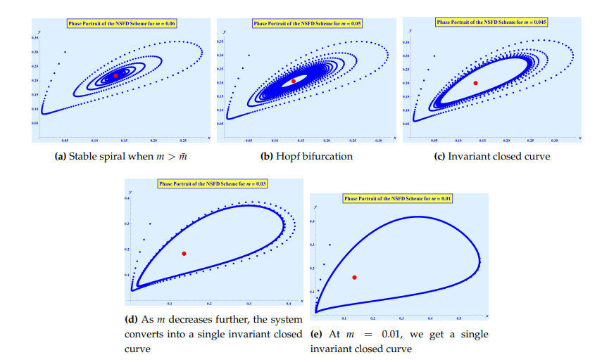
Here, we take \(m\) as the bifurcation parameter. Let us assume that \(\left(\alpha, \beta, \delta, \bar{m}, \gamma, \rho, k\right)\) \(=\) \(\left(0.6, 0.35, 0.49, 0.0504637, 0.2, 0.8, 0.5\right)\), \(m \in [0.001, 0.1]\) and the initial value \((x_0, y_0) = (0.05, 0.3)\). The Jacobian matrix is \[\left( \begin{array}{cc} \dfrac{0.949308 \bar{m}^2 + 0.303865 \bar{m} + 0.0300235}{\bar{m}^2 + 0.317624 \bar{m} + 0.0246878} & – \dfrac{0.0304155}{\bar{m} + 0.18191} \\ \dfrac{0.0052519}{\left(\bar{m} + 0.158423\right)^2} & \dfrac{1.12198 \left(\bar{m}+0.135714\right)^2}{\left(\bar{m}+0.158423\right)^2} \\ \end{array} \right),\] and for \(m = \bar{m} = 0.0504637\) the eigenvalues are\(\nu_1 = 0.997792 – 0.0664121\iota\) and \(\nu_2 = 0.997792 + 0.0664121\iota\). Both eigenvalues have norm equal to \(1\). Note that, \(\mathbb{T}(0) = 19.1813 \neq 0\) and \(\mathbb{T}(1) = 2.56518 \neq 0\), thus, \(\mathbb{T}(m_0) = 1.99558 \notin \left\{-2, 0, 1, 2\right\}\), Also, \(\mathbb{D}(m_0 ) = 1\), \(\dfrac{1-2 \bar{x}-\gamma -m}{\bar{x}+m} \in \left(-\dfrac{B+3}{A_1}, \dfrac{1-B}{A_1}\right)\) and \(\left(\dfrac{d\left|\nu_{1}\right|}{d \bar{m}}\right)_{\bar{m}=0} = \left(\dfrac{d\left|\nu_{2}\right|}{d \bar{m}}\right)_{\bar{m}=0} = 4.11006 \neq 0\). Finally, we get, \(\mho = -87574 \neq 0\). Thus, the fixed point exhibits Neimark-Sacker bifurcation, at the fixed point \(\left(\bar{x}, \bar{y}\right)\) \(=\) \(\left(0.135714,0.206126\right)\), as can be seen in Figure 5. Furthermore, for \(m > 0.0504637\), we have \(\mho < 0\) and an invariant closed curve bifurcates from the fixed point which is attracting.
The stable fixed point will become unstable due to Neimark-Sacker bifurcation on varying the parameter \(m\) above the threshold value \(0.0504637\). In Figure 6a at \(m = 0.06\), the fixed point is a stable spiral point and as \(m\) decreases, the stable spiral looses its stability. The spiral becomes dense and eventually breaks as \(m\) gets closer to the threshold value \(0.0504637\). At this point the stable spiral starts converting into an attracting invariant closed curve when \(m = 0.05\) and \(m = 0.045\) as can be seen in Figure 6b and Figure 6c respectively. In all these figures, the fixed point is represented by red dot. As is evident from the Figure 6d, as \(m\) is decreasing, the system behavior is converting gradually into a single attracting invariant closed curve. The Neimark-Sacker bifurcations is producing the quasi-periodic motions around the fixed point, which is obvious if we observe changes in phase portraits from small changes in the values of \(m\). In Figure 6e, the system has been converted to a single attracting invariant closed curve.

In this section, we apply multiple feedback control strategies to try controlling the chaos present in the both standard finite difference model (2) and the non-standard finite difference model propose in (14). To control the period-doubling bifurcation, we will apply the State Feedback Control method. In order to control the Neimark-Sacker bifurcations for both systems (2) and (14), we will use hybrid feedback control strategy which is shown to control Neimark-Sacker bifurcation, although initially its design was aiming to control the period-doubling bifurcation.
To control the chaotic behavior of system (2) around the period-doubling bifurcation, we apply the state feedback control method. Suppose that we introduce \(u_n = -S_1 \left(x_n – 0.215097\right) – S_2 \left(y_n – 0.705589\right)\) as feedback in the system 2. The new system is then given by: \[\label{SFC-disc-sys} \begin{cases} x_{n+1} = x_n + k x_n\left(1 – x_n – \dfrac{\alpha y_n}{m + x_n} – \gamma\right) + u_n, \\ y_{n+1} = y_n + k y_n \left(\rho \left(1 – \dfrac{\beta y_n}{m + x_n}\right) – \delta\right). \end{cases} \tag{20}\]
The Jacobian matrix \(J\) of the controlled system (20) evaluated at the interior fixed point \(\left(\bar{x}, \bar{y}\right)\) is given by: \[\left( \begin{array}{cc} 0.7661 – S_1 & -S_2 – 0.0118 \\ 1.0005 & -1.0067 \\ \end{array} \right).\]
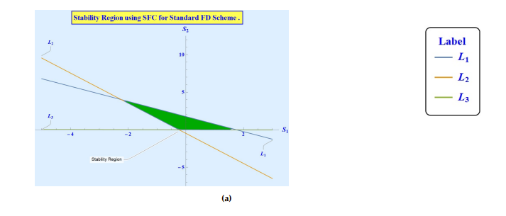
The trace and determinant of the above matrix are \(-0.2406 – S_1\) and \(1.0067 S_1 + 1.0005 S_2 – 0.7593\) respectively. Thus, the lines of marginal stability are as follows: \[\label{eq:SD-SFC-margLines} \begin{cases} l_1 : S_2 = -1.006 S_1 + 1.7583 , \\ l_2 : S_2 = -2.0055 S_1 – 0.4809,\\ l_3 : S_2 = -0.0067 S_1 – 1.3314\times10^{-15}. \end{cases} \tag{21}\]
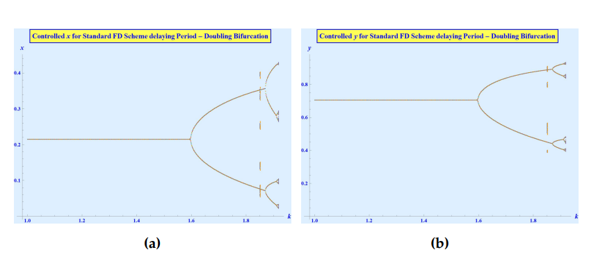
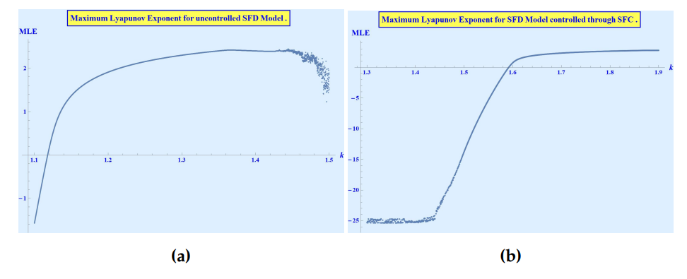
The region shown in Figure 7 is the one bounded by the marginal stability lines given in (21) and represents the combinations of \(S_1\) and \(S_2\) for which the period-doubling bifurcation of the system (2) is delayed to \(k = 1.6\) instead of \(k = 1.11484\). And even after \(k = 1.6\), it can be seen in Figure 8 that the chaotic orbits are very much controlled and not getting out of control as was the case in the uncontrolled system. This is also confirmed by looking at the Maximum Lyapunov exponents in the Figure 9 where the comparison between the Maximum Lyapunov exponents around the period-doubling bifurcation of the uncontrolled system (2) \((S_1 = S_2 = 0)\) and the controlled system (20), where \(S_1\) and \(S_2\) belongs to the stability region shown in Figure 7 is shown. This comparison shows that the MLE is delayed to enter the positive region and not until \(k\) reaches near \(1.6\) that we see the evidence of chaotic behavior in the system.
Let \(\left(\alpha, \beta, \delta, m, \gamma, \rho\right)\) \(=\) \(\left(1, 0.6, 0.3, 0.1, 0.3, 0.4\right)\), \(k \in [2.2, 5.2]\) and the initial value \((x_0, y_0) = \left(0.4, 0.1\right)\). As shown in example 2.4.1 the system (2) exhibits Neimark-Sacker bifurcation around \(k = 2.65\). To control the chaotic behavior of system (2) we apply the hybrid feedback control method. For that purpose, lets modify system (2) as follows: \[\label{SFC-NS-CSystem} \begin{cases} x_{n+1} = \xi\left(x_n + k x_n\left(1 – x_n – \dfrac{\alpha y_n}{m + x_n} – \gamma\right)\right) + \left(1-\xi\right)x_n, \\ y_{n+1} = \xi\left(y_n + k y_n \left(\rho \left(1 – \dfrac{\beta y_n}{m + x_n}\right) – \delta\right)\right) + \left(1-\xi\right)y_n, \end{cases} \tag{22}\] where \(\xi \in [0, 1]\) and the controlled strategy in the above system is a combination of both parameter perturbation and feedback control. Moreover, by suitable choice of controlled parameter \(\xi\), the period-doubling bifurcation and Neimark-Sacker bifurcation for the equilibrium point \(\left(\bar{x}, \bar{y}\right)\) of the controlled system above, can be advanced (delayed) or even completely eliminated. The variational matrix of controlled system, determined at \(\left(\bar{x}, \bar{y}\right)\) is: \[\left( \begin{array}{cc} 0.0655325 \xi +1 & -1.96597 \xi \\ 0.110827 \xi & 0.734015 \\ \end{array} \right).\]
If we define the trace and the determinant of the above matrix as \(\tau_2\) and \(\Delta_2\) respectively, then: \[\begin{aligned} \tau_2 &=& 0.0655325 \xi +1.73402, \\ \Delta_2 &=& 0.217883 \xi^2 + 0.0481018 \xi + 0.734015. \end{aligned}\]
The controlling affect is apparent in Figure 10. For \(\xi = 1\), i-e, for the original system (2) the behavior of \(x\), \(y\) and the complete system is shown in figures 10\((a)\), (10)\((c)\) and (10)\((e)\) respectively. The system is showing chaotic behavior. To control it, let \(\xi = 0.93\). Then the system starts behaving in a very controllable manner as is evident from the figures in 10\((b)\), 10\((d)\) and 10\((f)\).
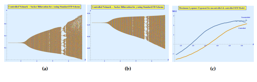
The resulting controlled bifurcation diagrams and the comparison of Maximum Lyapunov exponents for the uncontrolled system (2) \((\xi = 1)\) and the controlled system (22) \(\xi = 0.8\) are given in Figures (11)\((a)\), (11)\((b)\) and (11)\((c)\), respectively. By looking at comparisons of MLEs, we can see that the chaos in the system is delayed from approximately \(k = 2.9\) to \(k = 3.65\). This information can also be verified in the bifurcation diagrams of the controlled system, which shows the efficiency of the control strategy.
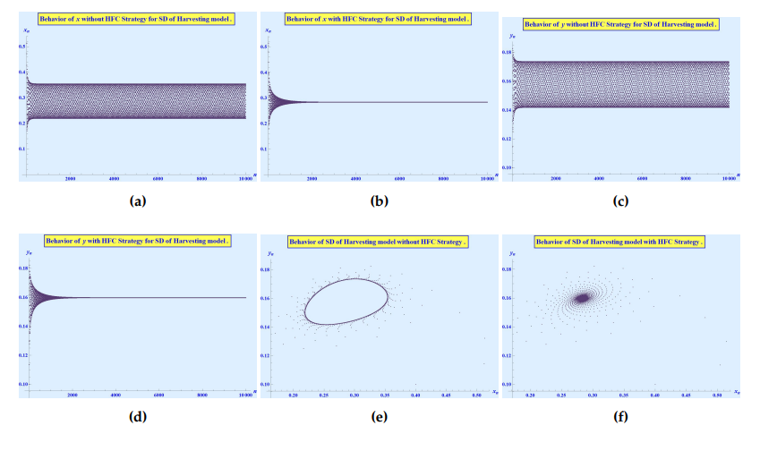
Let \(\left(\alpha, \beta, \delta, m_0, \gamma, \rho, k\right)\) \(=\) \(\left(0.6, 0.35, 0.49, 0.0504, 0.2, 0.8, 0.5\right)\) and the initial value \((x_0, y_0) = \left(0.05, 0.3\right)\). As shown in example 3.2.1 the system (12) exhibits Neimark-Sacker bifurcation around \(m = m_0\). To control the chaotic behavior of system (12) we apply the hybrid feedback control method. For that purpose, lets modify system (12) as follows. \[\label{HFC-NSFD-CSystem} \begin{cases} x_{n+1} = \xi\left( \dfrac{\left(1 + (1-\gamma ) \phi(k)\right) x_n}{1 + \phi(k)\left(\dfrac{\alpha y_n}{m+x_n}+x_n\right)}\right) + \left(1-\xi\right)x_n ,\\ y_{n+1} = \xi\left(\dfrac{\left(1 + \phi(k)(\rho -\delta )\right)y_n}{1 + \dfrac{\phi(k)(\beta \rho y_n)}{m+x_n}}\right) + \left(1-\xi\right)y_n, \end{cases} \tag{23}\] where \(\xi \in [0, 1]\) and the controlled strategy in the above system is a combination of both parameter perturbation and feedback control. It is obvious as well that the more \(\xi\) is close to \(1\), the less control is exerted on the system for chaos. The closer \(\xi\) is to \(0\), it means the chaos is not controllable through light control actions. Moreover, by suitable choice of controlled parameter \(\xi\), the period-doubling bifurcation and Neimark-Sacker bifurcation for the equilibrium point \(\left(\bar{x}, \bar{y}\right)\) of the controlled system above, can be advanced (delayed) or even completely eliminated. The variational matrix of controlled system, determined at \(\left(\bar{x}, \bar{y}\right)\) is: \[\left( \begin{array}{cc} 0.104299 \xi +1 & -0.13089 \xi \\ 0.120363 \xi & 1-0.108715 \xi \\ \end{array} \right).\]
If we define the trace and the determinant of the above matrix as \(\tau_3\) and \(\Delta_3\) respectively, then: \[\begin{aligned} \tau_3 &=& 2 – 0.00441544 \xi ,\\ \Delta_3 &=& 0.0044 \xi^2 – 0.0044 \xi + 1. \end{aligned}\]
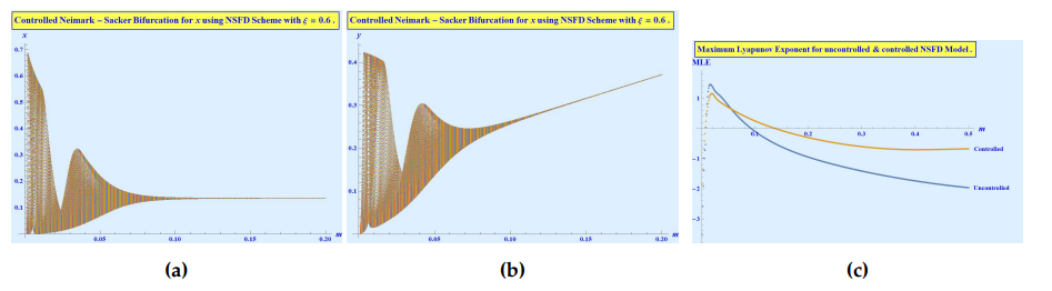
The controlling affect is apparent in Figure12. In fact we can see that the system is quite unstable when the parameter \(m\) passes the threshold value of \(m_0\) and to control the system or to delay the bifurcation, we have to change the value of our control parameter \(\xi\) now and again. As an example, when \(m = 0.0504\) the system starts exhibiting the Neimark-Sacker bifurcation as is evident in Figure 12\((a)\). Note that in this figure and all the subsequent figures, when we take \(\xi = 1\) then we recover our uncontrolled system given in (12). Thus Figure 12\((a)\), Figure 12\((c)\) and Figure 12\((e)\) represents the behavior of uncontrolled system (12) for various values of the parameter \(m\). Thus at \(m = 0.0504\) the Neimar-Sacker bifurcations is delayed if we choose \(\xi = 0.97\) as is shown in Figure 12\((b)\). But as we reduce the value of \(m\) from \(0.0504\) to \(0.0495\), this value of \(\xi\) is not enough to delay the bifurcation. Instead the system keeps on exhibiting the emergence of Neimark-Sacker bifurcation. The system also shows in Figure 12\((c)\) the increase in the bifurcation activity. Thus in order to control the system at this stage, we need to decrease the value of \(\xi\) to \(0.8\). By doing so, as we can see in Figure 12\((d)\), the system’s state returns to pre-Neimark-Sacker behavior. The similar type of behavior is observable if we further decrease the value of \(m\) to \(0.0485\). The uncontrolled system’s chaotic behavior increase as shown in Figure 12\((e)\). Also no previously selected value of \(\xi\) is good enough to control this much chaos in the uncontrolled system. Due to which we have to further decrease the value of \(\xi\) to \(0.6\) to bring the controlled system to the pre-Neimark-Sacker stage. This is shown in Figure 12\((f)\). The resulting controlled bifurcation diagrams and the comparison of Maximum Lyapunov exponents for the uncontrolled system (14) \((\xi = 1)\) and the controlled system (23) \(\xi = 0.6\) are given in Figures (13)\((a)\), (13)\((b)\) and (13)\((c)\), respectively.

This paper studied the behavior of discrete Leslie-Gower type model with harvesting. The discretization of the continuous system has been done using initially the classical finite difference method (Forward Euler method). Then we designed a non-standard finite difference scheme for the system which is dynamically consistent and the best finite difference scheme, according to Mickens [39]. For both schemes, stability of fixed points and their topology has been discussed. It is shown that the forward Euler scheme do not change the fixed points of its continuous counterpart but changes their stability by introducing non-existent bifurcations and chaos in the system. While non-standard finite difference scheme changes neither. In the subsequent sections, the bifurcation scenarios for the unique positive interior fixed point of both schemes have been studied and proved, using the center limit theorem. We note that the non-standard finite difference scheme exhibits only the Neimark-Scaker bifurcation which leads to the stable limit cycles, as is the case with system (1). On the other hand, the discretization of system (1) using forward Euler method exhibits the period-doubling bifurcation as well as the Neimark-Sacker bifurcation. Also, this classical discretization scheme introduces chaos in the system, which is not inherent in the system and is because of the nature of the classical discretization process. We have also studied the chaos and its control for the both the systems and the bifurcations. The controlling effects are also shown.
The mathematical results are supported with some numerical examples showing the period-doubling bifurcation in Example 2.3.1 and Neimark-Sacker bifurcation in Example 2.4.1 for system (2) and the Neimark-Sacker bifurcation in Example 3.2.1 for system (12). Using Mathematica®, we carry out the numerical simulations to support the analytical results obtained in sections §2.3, §2.4 and §3.2. The numerical simulations reaffirm our analytical results, while displaying insights about the local stability of the positive interior fixed point. As is known already, a slight change in the parametric values, change the behavior of the system’s trajectories, which makes its dynamics more complex. By using different values of parameters \(\left(\alpha, \beta, \delta, m, \gamma, \rho, k\right)\), we numerically showed the presence of period-doubling and Neimark-Sacker bifurcations for system (2) and the Neimark-Sacker bifurcation for system (12). Theese numerical results are supported by the phase portraits at different values of bifurcation parameter and the bifurcations diagrams. Based on the result in this study, harvesting firms have better chance of maximizing their gains by setting their constraints to a certain value while varying them from time to time according to the stability conditions.