
Periodic motion is a naturally occurring phenomenon in many physical processes [1]. It is a motion that repeats itself at equal time intervals, such as the oscillation of a pendulum or the Earth’s orbit around the Sun. The time interval at which the motion repeats is called the period, while the number of periods per unit of time is called the frequency.
A special case of periodic motion is simple harmonic motion, in which the motion occurs in a regular, sinusoidal manner. Periodic motion can be observed in a wide range of forms, from the oscillation of a pendulum to spectacular planetary orbits, as well as the vibrations of waves and enzymatic reactions in biochemical systems. The latter are usually modeled by ordinary differential equations (ODEs) or partial differential equations (PDEs), which are classified based on their order, linearity, and other properties [2– 7].
Several methods can be used to study the existence of periodic solutions of differential equations, including the method of guiding functions, the fixed point theorem, topological degree, bifurcation theory, and the Lyapunov function method. These methods are employed to prove the existence of periodic solutions for various types of differential equations, including ordinary differential equations (ODEs) and partial differential equations (PDEs) [8].
Classical studies of cooperative differential systems typically assume that the data are only bounded and smooth (\(L^{\infty}\) or continuous data), ensuring the existence of strong T-periodic solutions via classical ODE methods. In contrast, the novelty of this work relies on considering a more general case where the data are only \(L^1\), a biologically relevant hypothesis, allowing for discontinuous, unbounded or even zero-tending source terms. The existence of T-periodic weak solutions is established in the Sobolev space \(W^{1,1}_{per}\) through the construction of ordered sub and super-solutions and the application of a regularizing operator \(K_{\lambda}\), which gives an explicit complete representation of the periodic solution. Contrast this with classical numerical approaches (e.g. Runge Kutta) that rely on known initial conditions; herein, the solution to the proposed system is constructed directly without prior knowledge of initial conditions. Thus, the proposed approach extends both functional framework and the solution notion for cooperative systems, preserving existence results.
In this study, a thorough mathematical analysis will be conducted to show the existence of a periodic solution for a generic cooperative system of order \(m \times m\), which is used to model real phenomena. An application example is provided, describing the dynamics of cell volume related to the transport of water and solutes across the cell membrane. §2 is devoted to mathematical preliminaries, where the definition and properties of the periodic differential kernel \(K_{\lambda}\) are given. The general cooperative system to be studied is then presented. In Section §3, it is shown that the existence of a weak periodic subsolution and a weak periodic supersolution implies the existence of a weak periodic solution. This criterion is quite general and can be extended to any cooperative system of periodic partial differential equation.
Let \(T>0\) be fixed and set \(I:=(0,T)\). For \(m\in\mathbb{N}\) we use the usual Banach spaces \[C_{\mathrm{per}}([0,T];\mathbb{R}^{m}) :=\{u\in C([0,T];\mathbb{R}^{m}) : u(0)=u(T)\},\] and \[W^{1,1}_{\mathrm{per}}(0,T;\mathbb{R}^{m}) :=\{u\in W^{1,1}(0,T;\mathbb{R}^{m}) : u(0)=u(T)\},\] endowed with their standard norms. On \(\mathbb{R}^{m}\), we use the componentwise order \[u\le v \quad\Longleftrightarrow\quad u_i\le v_i \ \text{for all }i=1,\dots,m.\]
For \(u,v\in C_{\mathrm{per}}([0,T];\mathbb{R}^{m})\) we then write \(u\le v\) if \(u(t)\le v(t)\) for every \(t\in[0,T]\).
We first recall the scalar periodic problem \[\label{eq:scalar-periodic} \begin{cases} u'(t)+\lambda u(t)=\sigma(t), & t\in I,\\[2mm] u(0)=u(T), \end{cases} \tag{1}\] where \(\lambda>0\) and \(\sigma\in L^{1}(0,T)\).
Lemma 1. Let \(\lambda>0\) and \(\sigma\in L^{1}(0,T)\).
(i) Problem (1) admits a unique solution \(u\in W^{1,1}_{\mathrm{per}}(0,T;\mathbb{R}^{m})\) given by \[\label{eq:Klambda-def} u(t)=\int_{0}^{T}K_{\lambda}(t,s)\,\sigma(s)\,ds, \qquad t\in[0,T], \tag{2}\] where \[\label{eq:Klambda-kernel} K_{\lambda}(t,s)= \frac{ e^{-\lambda(t-s)}}{1- e^{-\lambda T}} \, {1}_{(0,t)}(s) + \frac{e^{-\lambda(t-s+T)}}{1- e^{-\lambda T}} \, {1}_{(t,T)}(s). \tag{3}\]
Equivalently, \[K_{\lambda}(t,s)= e^{-\lambda(t-s)} {1}_{(0,t)}(s) + \frac{e^{\lambda(s-t)}}{e^{\lambda T}-1},\] which is nonnegative for all \(t,s \in (0,T)\). In the following, we denote this T-periodic solution by \(u=K_{\lambda}(\sigma)\).
(ii) The operator \[K_{\lambda}:L^{1}(0,T)\longrightarrow W^{1,1}_{\mathrm{per}}(0,T;\mathbb{R}^{m}) \hookrightarrow C_{\mathrm{per}}([0,T];\mathbb{R}^{m}),\] is linear and continuous, and the embedding into \(C_{\mathrm{per}}([0,T];\mathbb{R}^{m})\) is compact.
Furthermore, a simple calculation shows that \[\sup_{t\in [0,T]} \sup_{s\in [0,T]}|K_{\lambda}(t,s)|= \dfrac{e^{\lambda T}}{e^{\lambda T}-1}.\]
This yields for all \(\sigma \in L^1(0,T)\): \[\label{eq:bound-Klambda} \|K_{\lambda}(\sigma)\|_{C([0,T])} \le \dfrac{e^{\lambda T}}{e^{\lambda T}-1}\,\|\sigma\|_{L^{1}(0,T)}. \tag{4}\]
(iii) \(K_{\lambda}\) is order preserving: if \(\sigma_{1},\sigma_{2}\in L^{1}(0,T)\) satisfy \(\sigma_{1}\le\sigma_{2}\) a.e., then \(K_{\lambda}(\sigma_{1})\le K_{\lambda}(\sigma_{2})\) on \([0,T]\).
(iv) For every \(\sigma\in L^{1}(0,T)\), \(u=K_{\lambda}(\sigma)\) is the unique element of \(W^{1,1}_{\mathrm{per}}(0,T;\mathbb{R}^{m})\) satisfying \[\label{eq:resolvent-identity} u'(t)+\lambda u(t)=\sigma(t)\quad\text{for a.e.\ }t\in I, \qquad u(0)=u(T). \tag{5}\]
Proof. (i) The computations are standard; we sketch them for completeness.
By integrating (1) over \((0,t)\), one gets \[u(t)e^{\lambda t}=u(0) + \int_{0}^{t}e^{\lambda s}\sigma(s)ds.\]
Since \(u(0)=u(T)\), we obtain for \(t=T\) \[u(0)e^{\lambda T}=u(0)+\displaystyle\int_{0}^{T}e^{\lambda s}\sigma(s)ds.\]
Thus \[u(0)=\dfrac{1}{e^{\lambda T}-1} \displaystyle\int_{0}^{T}e^{\lambda s}\sigma(s)ds.\]
Substituting back, \[u(t)=u(0)e^{-\lambda t} +\displaystyle\int_{0}^{t}e^{-\lambda (t-s)}\sigma(s)ds.\]
After simplification, we get \[u(t)=\displaystyle\int_{0}^{T}K_{\lambda}(t,s)\sigma(s)ds,\] with \[\label{Kernel} K_{\lambda}(t,s)= \frac{ e^{-\lambda(t-s)}}{1- e^{-\lambda T}} \, {1}_{(0,t)}(s) + \frac{e^{-\lambda(t-s+T)}}{1- e^{-\lambda T}} \, {1}_{(t,T)}(s).\]
The equivalent form is \[K_{\lambda}(t,s)= e^{-\lambda(t-s)} {1}_{(0,t)}(s) + \frac{e^{\lambda(s-t)}}{e^{\lambda T}-1}.\] Since \(\lambda, \ T>0\), \(K_{\lambda}(t,s)\geq 0\) for all \(t,s\).
(iii) Let \(\sigma_1, \ \sigma_2\in L^1(0,T)\), such that \(\sigma_2(s)-\sigma_1(s)\geq 0 \text{ a.e } s\in]0,T[\). By using the linearity of \(K_{\lambda}\), we obtain \[K_{\lambda}(\sigma_2)(t)-K_{\lambda}(\sigma_1)(t)=K_{\lambda}(\sigma_2-\sigma_1)(t) =\int_{0}^{T}K_{\lambda}(t,s)[\sigma_2(s)-\sigma_1(s)]\,ds.\]
Since \(K_{\lambda}(t,s)\geq 0\) for all \(t,s\in[0,T]\), then \(K_{\lambda}(\sigma_1)(t)\le K_{\lambda}(\sigma_2)(t)\) for all \(t\).
Items (ii) and (iv) follow by direct estimates and the uniqueness of solutions to the linear ODE. ◻
We now consider the \(m\times m\) nonlinear periodic system \[\label{eq:main-system} \begin{cases} u_i'(t) = f_i\bigl(t,u_1(t),\dots,u_m(t)\bigr) + F_i(t), & t\in I,\ i=1,\dots,m,\\[1mm] u_i(0)=u_i(T),& i=1,\dots,m, \end{cases} \tag{7}\] where \(F_i\in L^{1}(0,T)\) and \(f_i:[0,T]\times D\to\mathbb{R}\), \(D\subset\mathbb{R}^{m}\) a bounded open set, satisfy the following Carathéodory/Nemytskii assumptions.
(A1) (Measurability and periodicity) For every \(r\in D\), the map \(t\mapsto f_i(t,r)\) is Lebesgue-measurable, \(T\)-periodic on \(\mathbb{R}\) and belongs to \(L^{1}(0,T)\).
(A2) (Pointwise regularity) For a.e. \(t\in(0,T)\), the map \(r\mapsto f_i(t,r)\) is \(C^{1}(D)\).
(A3) (Cooperativity) For all \(r\in D\), \(i\neq j\) and a.e. \(t\in(0,T)\), \[\frac{\partial f_i}{\partial r_j}(t,r)\ge0.\]
(A4) (Local growth) For every compact \(B\subset D\) there exists \(\varphi_B\in L^{1}(0,T)\) such that \[|f(t,r)|\le \varphi_B(t) \quad\text{for all }r\in B\text{ and a.e.\ }t\in(0,T),\] where \(f=(f_1,\dots,f_m)\).
Assumption (A4) ensures that the associated Nemytskii operator \[N_f : C_{\mathrm{per}}([0,T];D)\longrightarrow L^{1}(0,T;\mathbb{R}^{m}), \qquad (N_f u)(t):=f(t,u(t)),\] is well defined and continuous.
Definition 1(Weak/Carathéodory \(T\)-periodic solution). Let \(F=(F_1,\dots,F_m)\in L^{1}(0,T;\mathbb{R}^{m})\) and suppose that (A1)–(A4) hold. A map \(u=(u_1,\dots,u_m)\in W^{1,1}_{\mathrm{per}}(0,T;\mathbb{R}^{m})\) with \(u(t)\in D\) for a.e. \(t\in(0,T)\) is called a weak (Carathéodory) \(T\)-periodic solution of (7) if \[u_i'(t) = f_i\bigl(t,u(t)\bigr)+F_i(t) \quad\text{for a.e.\ }t\in(0,T),\quad i=1,\dots,m,\]
In this section we work in the ordered Banach space \(C_{\mathrm{per}}([0,T];\mathbb{R}^{m})\) endowed with the componentwise order introduced above.
Definition 2(sub- and supersolutions).Let \(F\in L^{1}(0,T;\mathbb{R}^{m})\) and suppose that (A1)–(A4) hold.
A vector \(\underline{u}=(\underline{u}_1,\dots,\underline{u}_m) \in W^{1,1}_{\mathrm{per}}(0,T;\mathbb{R}^{m})\) with \(\underline{u}(t)\in D\) a.e. is called a weak \(T\)-periodic subsolution of (7) if \[\underline{u}_i'(t) \le f_i\bigl(t,\underline{u}(t)\bigr)+F_i(t) \quad\text{for a.e.\ }t\in(0,T), \qquad i=1,\dots,m.\]
Similarly, \(\overline{u}=(\overline{u}_1,\dots,\overline{u}_m) \in W^{1,1}_{\mathrm{per}}(0,T;\mathbb{R}^{m})\) with \(\overline{u}(t)\in D\) a.e. is called a weak \(T\)-periodic supersolution of (7) if \[\overline{u}_i'(t) \ge f_i\bigl(t,\overline{u}(t)\bigr)+F_i(t) \quad\text{for a.e.\ }t\in(0,T), \qquad i=1,\dots,m.\]
We say that \((\underline{u},\overline{u})\) is an ordered pair of barriers if \(\underline{u}(t)\le\overline{u}(t)\) for all \(t\in[0,T]\).
For an ordered pair of barriers \((\underline{u},\overline{u})\), we define the order interval \[[\underline{u},\overline{u}] :=\bigl\{v\in C_{\mathrm{per}}([0,T];\mathbb{R}^{m}) : \underline{u}(t)\le v(t)\le\overline{u}(t)\ \forall t\in[0,T]\bigr\}.\]
We now introduce the key structural hypothesis controlling the diagonal derivatives of \(f_i\) inside the order interval.
(H\(_\lambda\)) \[\exists \lambda>0 \text{ s.t. }\forall t \in[0, T], \forall r \in D \ \text{ with } \underline{u}(t) \leq r \leq \bar{u}(t):\left|\frac{\partial f_i}{\partial r_i}(t, r)\right| \leq \lambda. \tag{8}\]
Under (A1)–(A4) and (H\(_\lambda\)), we can define the nonlinear operator \[\mathcal{T}:[\underline{u},\overline{u}]\longrightarrow C_{\mathrm{per}}([0,T];\mathbb{R}^{m}),\] componentwise by \[\label{eq:T-operator} (\mathcal{T}u)_i :=K_{\lambda}\bigl(f_i(\cdot,u(\cdot))+\lambda u_i(\cdot)+F_i(\cdot)\bigr), \quad i=1,\dots,m. \tag{9}\]
Lemma 2(Order preserving and invariance of the interval).Assume (A1)–(A4) and (H\(_\lambda\)) and let \((\underline{u},\overline{u})\) be an ordered pair of weak sub- and supersolutions of (7) in the sense of Definition 2. Then:
(i) \(\mathcal{T}\) maps the interval into itself, \[\mathcal{T}\bigl([\underline{u},\overline{u}]\bigr) \subset [\underline{u},\overline{u}].\]
(ii) \(\mathcal{T}\) is order preserving: if \(u,v\in[\underline{u},\overline{u}]\) with \(u\le v\), then \(\mathcal{T}u\le \mathcal{T}v\).
(iii) \(\mathcal{T}\) is completely continuous (continuous with relatively compact range).
Proof. (i) Invariance of \([\underline{u},\overline{u}]\). Let \(u\in[\underline{u},\overline{u}]\) be fixed and set \[w_i(t):=(\mathcal{T}u)_i(t)-\underline{u}_i(t).\]
Using the linearity of \(K_{\lambda}\), Lemma 1, and the fact that by Definition 2 we have \(f_i(t,\underline{u}(t))+F_i(t)-\underline{u}_i'(t)\ge0\), we obtain \[w_i \geq K_{\lambda}\bigl(f_i(\cdot,u)-f_i(\cdot,\underline{u})+\lambda (u_i – \underline{u}_i\bigr)).\]
Now using (H\(_\lambda\)), we get \[f_i(\cdot,u)-f_i(\cdot,\underline{u}))+\lambda (u_i – \underline{u}_i\bigr) \geq 0 \quad\text{for a.e.\ }t.\]
It follows that \(w_i\ge0\) on \([0,T]\), so \((Tu)_i\ge\underline{u}_i\).
Similarly, setting \(z_i(t):=(Tu)_i(t)-\overline{u}_i(t)\), we obtain \[z_i \leq K_{\lambda}\bigl(f_i(\cdot,u)-f_i(\cdot,\overline{u})+\lambda (u_i – \overline{u}_i\bigr)).\]
By using (H\(_\lambda\)), we get \[f_i(\cdot,u)-f_i(\cdot,\overline{u}))+\lambda (u_i – \overline{u}_i\bigr) \leq 0 \quad\text{for a.e.\ }t,\]
Therefore \(z_i\le0\) on \([0,T]\). Hence \(Tu\le\overline{u}\) and (i) follows.
(ii) Order preserving. Let \(u,v\in[\underline{u},\overline{u}]\) with \(u\le v\). We compute, for each \(i\), \[\begin{aligned} (\mathcal{T}v)_i-(\mathcal{T}u)_i &=K_{\lambda}\bigl(f_i(\cdot,v)-f_i(\cdot,u) +\lambda(v_i-u_i)\bigr). \end{aligned}\]
Fix \(t\in(0,T)\) and set \(\delta(t):=v(t)-u(t)\ge0\). By (A2), one can write \[f_i(t,v(t))-f_i(t,u(t)) =\int_{0}^{1} \sum_{\substack{j=1 \\ j \neq i}}^{m } \frac{\partial f_i}{\partial r_j}\bigl(t,u(t)+\theta\delta(t)\bigr)\cdot\delta(t)\,d\theta + \int_{0}^{1} \frac{\partial f_i}{\partial r_i}\bigl(t,u(t)+\theta\delta(t)\bigr)\cdot\delta(t)\,d\theta .\]
Using cooperativity (A3) and the bound (H\(_\lambda\)) on the diagonal derivative, we obtain \[\bigl(f_i(t,v(t))-f_i(t,u(t))\bigr) +\lambda\delta_i(t) \ge0 \quad\text{for a.e.\ }t\in(0,T).\]
Thus \[f_i(\cdot,v)-f_i(\cdot,u)+\lambda(v_i-u_i)\ge0 \quad\text{a.e. on }(0,T),\] and Lemma 1(iii) yields \((\mathcal{T}v)_i-(\mathcal{T}u)_i\ge0\) on \([0,T]\). Hence \(\mathcal{T}u\le \mathcal{T}v\).
(iii) Complete continuity. By (A4) and the boundedness of \([\underline{u},\overline{u}]\) in \(C_{\mathrm{per}}([0,T];\mathbb{R}^{m})\), the set \(\{f(\cdot,u(\cdot))+F(\cdot):u\in[\underline{u},\overline{u}]\}\) is bounded in \(L^{1}(0,T;\mathbb{R}^{m})\). Lemma 1(ii) implies that \(K_{\lambda}\) maps bounded sets of \(L^{1}\) into relatively compact subsets of \(C_{\mathrm{per}}([0,T];\mathbb{R}^{m})\), and the continuity of the Nemytskii operator (A1)–(A4) yields the continuity of \(\mathcal{T}\). ◻
We can now state the main existence result.
Theorem 1(Existence of a weak periodic solution).Assume (A1)–(A4) and (H\(_\lambda\)). Suppose that the system (7) admits a pair of weak \(T\)-periodic sub- and supersolutions \(\underline{u},\overline{u}\in W^{1,1}_{\mathrm{per}}(0,T;\mathbb{R}^{m})\) with \(\underline{u}\le\overline{u}\). Then there exists at least one weak \(T\)-periodic solution \(u\in W^{1,1}_{\mathrm{per}}(0,T;\mathbb{R}^{m})\) of(7) such that \[\underline{u}(t)\le u(t)\le\overline{u}(t) \quad\text{for all }t\in[0,T].\]
Proof. Let \(\mathcal{T}\) be the operator defined in (9). By Lemma 2 we know that \(\mathcal{T}\) is order preserving, completely continuous and leaves the interval \([\underline{u},\overline{u}]\) invariant.
Define the monotone sequence \((u^{n})_{n\ge0}\subset [\underline{u},\overline{u}]\) by \[u^{0}:=\underline{u},\qquad u^{n+1}:=Tu^{n},\ n\ge0.\]
By Lemma 2(i)–(ii) we have \[\underline{u}=u^{0}\le u^{1}\le u^{2}\le\cdots\le\overline{u}.\]
Since \(\mathcal{T}\) is completely continuous, the set \(\mathcal{T}([\underline{u},\overline{u}])\) is relatively compact in \(C_{\mathrm{per}}([0,T];\mathbb{R}^{m})\), and therefore \((u^{n})_{n\ge1}\) is relatively compact. Because \((u^{n})\) is monotone in the order of \(C_{\mathrm{per}}([0,T];\mathbb{R}^{m})\) and bounded by \(\overline{u}\), there exists \(u\in C_{\mathrm{per}}([0,T];\mathbb{R}^{m})\) such that \(u^{n}\to u\) uniformly on \([0,T]\).
By the continuity of \(T\) we have \[u^{n+1}=\mathcal{T}u^{n}\longrightarrow \mathcal{T}u \quad\text{in }C_{\mathrm{per}}([0,T];\mathbb{R}^{m}),\] while the left-hand side converges to \(u\), so \(u=Tu\). Hence, for each \(i=1,\dots,m\), \[u_i =K_{\lambda}\bigl(f_i(\cdot,u)+\lambda u_i+F_i\bigr) \quad\text{on }[0,T].\]
Using Lemma 1(iv) with \[\sigma_i:=f_i(\cdot,u)+\lambda u_i+F_i\in L^{1}(0,T),\] we obtain \[u_i'(t)+\lambda u_i(t)=\sigma_i(t) =f_i\bigl(t,u(t)\bigr)+\lambda u_i(t)+F_i(t) \quad\text{for a.e.\ }t\in(0,T),\] so that \[u_i'(t)=f_i\bigl(t,u(t)\bigr)+F_i(t) \quad\text{for a.e.\ }t\in(0,T),\] and \(u_i(0)=u_i(T)\) by Lemma 1. Thus \(u\) is a weak \(T\)-periodic solution of (7) in the sense of Definition 1, and by construction \(\underline{u}\le u\le\overline{u}\) on \([0,T]\). ◻
Under the same assumptions, the monotone scheme yields extremal periodic solutions in the order interval.
Theorem 2(Minimal and maximal periodic solutions).Assume (A1)–(A4) and (H\(_\lambda\)), and let \(\underline{u},\overline{u}\) be an ordered pair of weak sub- and supersolutions of (7). Define \[u^{0}:=\underline{u},\quad u^{n+1}:=\mathcal{T}u^{n}, \qquad v^{0}:=\overline{u},\quad v^{n+1}:=\mathcal{T}v^{n}.\]
Then:
(i) \((u^{n})_{n\ge0}\) increases and converges in \(C_{\mathrm{per}}([0,T];\mathbb{R}^{m})\) to a solution \(u_{*}\) of (7) with \(\underline{u}\le u_{*}\le\overline{u}\).
(ii) \((v^{n})_{n\ge0}\) decreases and converges in \(C_{\mathrm{per}}([0,T];\mathbb{R}^{m})\) to a solution \(u^{*}\) of (7) with \(\underline{u}\le u^{*}\le\overline{u}\).
(iii) \(u_{*}\) is the minimal and \(u^{*}\) the maximal \(T\)-periodic solution of (7) in the order interval \([\underline{u},\overline{u}]\); that is, if \(w\) is any other \(T\)-periodic solution with \(\underline{u}\le w\le\overline{u}\), then \(u_{*}\le w\le u^{*}\).
Proof. The monotonicity and convergence of \((u^{n})\) have already been proved in Theorem 1; the same argument applied to \((v^{n})_{n\ge0}\) yields a decreasing sequence converging to a fixed point \(u^{*}\) of \(T\) in \([\underline{u},\overline{u}]\).
If \(w\) is any other fixed point of \(\mathcal{T}\) in \([\underline{u},\overline{u}]\), we have by Lemma 2 \[\underline{u}=u^{0}\le w\le v^{0}=\overline{u}.\]
Assume inductively that \(u^{n}\le w\le v^{n}\). Then \[u^{n+1}=\mathcal{T}u^{n}\le \mathcal{T}w=w\le \mathcal{T}v^{n}=v^{n+1},\] and the claim follows by induction for all \(n\). Passing to the limit in \(n\) we obtain \(u_{*}\le w\le u^{*}\). ◻
For uniqueness (and, consequently, stability) within the order interval, we add a standard Lipschitz condition.
(A5) There exists \(L>0\) such that for a.e. \(t\in(0,T)\) and all \(r,s\in D\), \[\max\limits_{1\leq i\leq m}|G_i(t,r)-G_i(t,s)| \le L\,|r-s|,\] where \(|\cdot|\) denotes the Euclidean norm in \(\mathbb{R}^{m}\), and \(G_i(t,r)=f_i(t,r)+\lambda r_i\).
Proposition 1(Uniqueness under a small Lipschitz constant).Assume (A1)–(A5) and (H\(_\lambda\)). Suppose that \[\label{eq:contraction-condition} L<\dfrac{1-e^{-\lambda T}}{T}, \tag{10}\] then \(\mathcal{T}\) is a strict contraction on \([\underline{u},\overline{u}]\), and consequently the system (7) admits a unique \(T\)-periodic solution in \([\underline{u},\overline{u}]\).
Proof. For \(u,v\in[\underline{u},\overline{u}]\) we estimate, for each \(i\), \[\begin{aligned} \|(\mathcal{T}u)_i-(\mathcal{T}v)_i\|_{C([0,T])} &\le \dfrac{e^{\lambda T}}{e^{\lambda T}-1} \bigl\|f_i(\cdot,u)-f_i(\cdot,v)+\lambda(u_i-v_i)\bigr\|_{L^{1}(0,T)}. \end{aligned}\]
Using (A5), we obtain \[\begin{aligned} \|(\mathcal{T}u)_i-(\mathcal{T}v)_i\|_{C([0,T])} &\le \dfrac{LTe^{\lambda T}}{e^{\lambda T}-1}\|u-v\|_{C([0,T];\mathbb{R}^{m})}. \end{aligned}\]
Taking the maximum over \(i\) and using (10) we obtain \[\|\mathcal{T}u-\mathcal{T}v\|_{C([0,T];\mathbb{R}^{m})} \le q\,\|u-v\|_{C([0,T];\mathbb{R}^{m})},\] with \(q:=\dfrac{TL}{1-e^{-\lambda T}} \in (0,1)\). Hence \(\mathcal{T}\) is a contraction and has a unique fixed point in \([\underline{u},\overline{u}]\), which is necessarily the unique \(T\)-periodic solution of (7) in that interval. ◻
Remark 1(Stability).If \(u\) is the unique \(T\)-periodic solution provided by Proposition 1, then every solution of the non-autonomous system (7) with initial data in \([\underline{u}(0),\overline{u}(0)]\) remains in the order interval and converges to \(u\) in \(C_{\mathrm{per}}([0,T];\mathbb{R}^{m})\) as \(t\to+\infty\). This follows from the cooperation property (A3) and the uniqueness of the periodic orbit by standard arguments of monotone dynamical systems.
We revisit the model describing the dynamics of the mass of solute \(u(t)\) and the volume of water \(v(t)\) inside a cell, governed by
\[\label{TWCM} \begin{cases} u'(t) = a(t) – d\,\dfrac{u(t)}{v(t)},\\[2mm] v'(t) = -b(t) + \dfrac{u(t)}{v(t)} + \dfrac{\gamma}{v(t)}, \end{cases} \quad t\in(0,T), \tag{11}\] where \(a,b\in C([0,T])\) are nonnegative \(T\)-periodic functions and \(d,\gamma>0\) are constants. We seek positive \(T\)-periodic solutions \((u,v)\).
We work in the following phase domain \(D\) which is an open bounded subset of \(\mathbb{R}^2\) containing \(\{(u,v)\in\mathbb{R}^{2} : 0\leq u_{*}\le u\leq u^{*},\ 0<v_{*}\le v\le v^{*}\}\), for suitable positive constants \(u_{*},u^{*},v_{*},v^{*}\) to be specified below. On \(D\), the right-hand side of (11) is smooth and cooperative, and the previous analysis applies.
Theorem 3(Existence of a positive periodic orbit).Let
\(a,b\in C([0,T])\) be \(T\)-periodic with \[0\le a(t)\le a_{\max},\qquad
0<b_{\min}\le b(t)\le b_{\max}
\quad\text{for all }t\in[0,T],\] where \(a_{\max}=\max\limits_{t\in[0,T]} a(t)\),
\(b_{\min}=\min\limits_{t\in[0,T]}
b(t)\), \(b_{\max}=\max\limits_{t\in[0,T]}
b(t)\).
Assume that \[\label{eq:cell-condition}
d\,b_{\min} > a_{\max}
\quad\text{and}\quad
b_{\max}>0. \tag{12}\]
Then there exist positive constants \(u_{*},u^{*},v_{*},v^{*}\) and an ordered pair of constant sub- and supersolutions \[(\underline{u},\underline{v})\equiv(u_{*},v_{*}), \qquad (\overline{u},\overline{v})\equiv(u^{*},v^{*}),\] such that \[0 \leq u_{*}\le u^{*},\qquad 0<v_{*}\le v^{*},\] and the system (11) admits at least one positive \(T\)-periodic solution \((u,v)\) satisfying \[u_{*}\le u(t)\le u^{*},\qquad v_{*}\le v(t)\le v^{*} \quad\text{for all }t\in[0,T].\]
Proof. We rewrite (11) in the abstract form (7) with \(m=2\) and \(F\equiv 0\). The right-hand side is cooperative and smooth on \((0,+\infty)\times(0,+\infty)\).
Construction of a subsolution. Let \(v_{*}>0\) and set \(\underline{u}(t)\equiv u_{*}:=0\), \(\underline{v}(t)\equiv v_{*}\). Then \(\underline{u}'=\underline{v}'\equiv0\), and \[\underline{u}'(t) – \biggl( a(t) – d\,\frac{\underline{u}(t)}{\underline{v}(t)}\biggr) = -a(t)\le0,\] for all \(t\). For the \(v\)-equation we get \[\underline{v}'(t) – \biggl(-b(t)+\frac{\underline{u}(t)}{\underline{v}(t)} +\frac{\gamma}{\underline{v}(t)}\biggr) = b(t)-\frac{\gamma}{v_{*}}.\]
Thus \((\underline{u},\underline{v})\) is a weak subsolution provided \[b(t)-\frac{\gamma}{v_{*}}\le0 \quad\text{for all }t,\] that is, \[v_{*}\le \frac{\gamma}{b_{\max}}.\]
Choose, for instance, \[v_{*}:=\frac{\gamma}{2b_{\max}},\] which satisfies the above inequality and yields a strictly positive lower bound for \(v\).
Construction of a supersolution. We now look for constants \(u^{*}>0\), \(v^{*}>v_{*}\) such that \((\overline{u},\overline{v})\equiv(u^{*},v^{*})\) is a supersolution. The inequalities \[\overline{u}'(t) \ge a(t)-d\,\frac{\overline{u}(t)}{\overline{v}(t)}, \qquad \overline{v}'(t) \ge -b(t)+\frac{\overline{u}(t)}{\overline{v}(t)} +\frac{\gamma}{\overline{v}(t)},\] reduce to \[0\ge a(t)-d\,\frac{u^{*}}{v^{*}}, \qquad 0\ge -b(t)+\frac{u^{*}+\gamma}{v^{*}}, \quad\text{for all }t\in[0,T],\] that is, \[\label{eq:super-ineqs} d\,\frac{u^{*}}{v^{*}}\ge a_{\max}, \qquad \frac{u^{*}+\gamma}{v^{*}}\le b_{\min}. \tag{13}\]
The second inequality in (13) is equivalent to \[u^{*}\le v^{*}b_{\min}-\gamma.\]
Combining this with the first inequality gives \[a_{\max} \le d\,\frac{u^{*}}{v^{*}} \le d\,\frac{v^{*}b_{\min}-\gamma}{v^{*}} = d\,b_{\min}-d\,\frac{\gamma}{v^{*}}.\]
Hence a sufficient condition for the existence of \(v^{*}>0\) is \[d\,b_{\min}-d\,\frac{\gamma}{v^{*}} \ge a_{\max},\] which is possible precisely when \(d\,b_{\min}>a_{\max}\), i.e. (12). In that case we can choose, for example, \[v^{*} :=\frac{2d\gamma}{d\,b_{\min}-a_{\max}}>0,\] which makes the right-hand side strictly larger than \(a_{\max}\). Then we define \[u^{*}:=\frac{1}{2}\bigl(v^{*}b_{\min}-\gamma\bigr)>0,\] so that both inequalities in (13) hold.
Application of the abstract result. The constants \(u_{*},u^{*},v_{*},v^{*}\) constructed above satisfy \[0=u_{*}\le u^{*},\qquad 0<v_{*}<v^{*},\] and the constant functions \((\underline{u},\underline{v})\) and \((\overline{u},\overline{v})\) are, respectively, a weak subsolution and a weak supersolution of (11). We can now apply Theorem 1 with \(m=2\) to conclude that there exists at least one weak \(T\)-periodic solution \((u,v)\in W^{1,1}_{\mathrm{per}}(0,T;\mathbb{R}^{2})\) with \[u_{*}\le u(t)\le u^{*},\qquad v_{*}\le v(t)\le v^{*} \quad\text{for all }t\in[0,T],\] which is strictly positive in both components. ◻
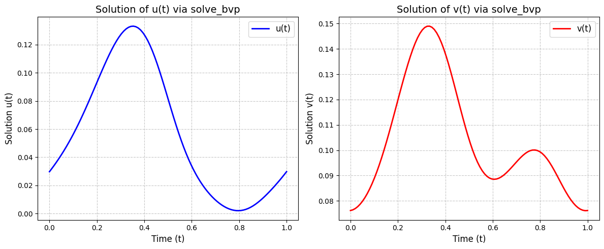
For illustration, take \(T=1\) and \[a(t)=1+ \sin(2\pi t), \qquad b(t)=2+\cos^2(2\pi t),\] so that \(a_{\max}=2\), \(b_{\min}=2\) , \(b_{\max}=3\). Let \(d=2\) and \(\gamma=0.2\). Then \[d\,b_{\min}=4>a_{\max}=2,\] so condition (12) holds. The construction above yields explicit constants \(u_{*},u^{*},v_{*},v^{*}>0\) and guarantees the existence of a strictly positive \(T\)-periodic solution \((u,v)\) to (11).
Biologically, \(u(t)\) represents the solute content and \(v(t)\) the cell volume. The inequalities \(u_{*}\le u(t)\le u^{*}\) and \(v_{*}\le v(t)\le v^{*}\) show that, under the given periodic forcing \(a(t)\) and \(b(t)\), the cell volume and solute mass oscillate in a bounded, strictly positive range, reflecting a periodic regime of osmotic regulation rather than collapse or unbounded swelling.
The algorithm for solving the following nonlinear periodic system 11 is implemented. The method used here is to directly calculate the periodic solution using the sequence defined in section (3). The fixed-point Algorithm 1 described below is then applied.
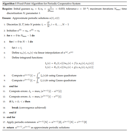
Where \(f(t,u,v)=a(t)-d \dfrac{u}{v},\) and \(g(t,u,v)= -b(t)+\dfrac{u}{v}+\dfrac{\gamma}{v}\), \(\lambda > 0\) is a fixed parameter, and \(K_{\lambda}\) represents the kernel given in Lemma 1.
This method is typically accurate, as the kernel inherently accounts for periodicity, thus eliminating the need for additional boundary condition calculations. However, it has certain drawbacks. The first limitation is the extended computation time, which is due to the complexity of the Gaussian quadrature required for integral calculations. Additionally, the choice of initial data and the value of \(\lambda\) are critical factors.
The following Figure 1 illustrates the solution obtained with \(\lambda=20\). The number of discretization points in \([0, 1]\) is \(N=100\), and \(\varepsilon_0=10^{-8}\). The computation time required was 2 minutes. This method is generally useful for comparison purposes.
Remark 2. (Convergence & sensitivity check) To verify numerical convergence, we performed mesh refinement tests with \(N \in \{50, 100, 200, 400\}\). The method provides consistent solutions for different discretizations when \(\lambda\) is sufficiently large. Also, the sensitivity to \(\lambda\) is tested, and optimal convergence is found for \(\lambda \in [20, 50]\).
With wide applicability to real-world models, this paper develops a generic criterion for the existence of periodic solutions in cooperative systems of dimension \(m \times m\). We have demonstrated the presence of a weak periodic solution by using the existence of weak periodic sub- and super-solutions. Based on the idea of the periodic differential kernel \(K_{\lambda}\), the framework created here is reliable and flexible enough to work with a variety of periodic ODE systems. The model’s applicability and potential for biological systems are demonstrated by its application to cellular volume dynamics. This method offers a useful tool for examining periodic behavior in applied contexts, in addition to advancing our theoretical understanding of cooperative systems.
All authors contributed equally to the writing of this paper. All authors read and approved the final manuscript.
This work does not have any conflicts of interest.