
| \(\mu_f\) | Fluid viscosity, \([kgm^{-1}s^{-1}]\) | \(Rd\) | Radiation parameter |
|---|---|---|---|
| \(\Omega^*\) | Volume expansion | \(g\) | Gravitational force |
| \(T_\infty\) | Ambient temperature | \(n_1,n_2\) | Velocity components in \(x\) and \(y\), \([ms^{-1}]\) |
| \(\sigma\) | Electrical conductivity, \([Sm^{-1}]\) | \(\chi\) | Dimensionless microorganism |
| \(\gamma^*\) | Microoganism average volume | \(x,~y\) | Dimensional space coordinates, \([m]\) |
| \(k_0\) | Initial permeability | \(Ec\) | Eckert number |
| \(\rho_m\) | Density of microoganism | \(Cf\) | Skin Friction |
| \(\rho_f\) | Fluid density, \([kgm^{-3}]\) | \(Pr\) | Prandtl number |
| \(\alpha\) | Thermal diffusivity, \([wn^{-1}k^{-1}]\) | \(\lambda\) | Ratio of heat capacitance to the base fluid |
| \(D_B\) | Brownian diffusion | \(r_2\) | Inertial parameter |
| \(D_T\) | Thermophoresis diffusion | \(r_1\) | Porosity parameter |
| \((Cp)_f\) | Specific heat capacity, \([Jkg^{-1}k^{-1}]\) | \(G_3\) | Rayleigh number |
| \(b\) | Chemotaxis coefficient | \(T\) | Temperature of fluid, \([k]\) |
| \(G_r\) | Grashof number | \(D_m\) | Nanoparticle diffusivity |
| \(k^*\) | Absorption coefficient | \(D_n\) | Microorganism diffusivity |
| \(\Theta\) | Dimensionless temperature, \([k]\) | \(\eta\) | Independent similarity variable |
| \(H\) | Dimensionless velocity | \(G\) | Concentration of microorganism |
| \(T_w\) | Temperature at wall, \([k]\) | \(N_b\) | Brownian motion parameter |
| \(\sigma^*\) | Boltzman fixed quantity | \(\varpi\) | Stream function |
| \(N_t\) | Thermophoresis parameter | \(Q\) | Heat production parameter |
| \(R_{ex}\) | Local Reynolds number | \(q_r\) | Radiation heat flux |
| \(\tau_w\) | Shear stress | \(q_w\) | Heat flux |
| \(fw\) | Suction/injection parameter | \(w_c\) | Cell moving speed |
| \(C\) | Concentration of nanoparticles | \(Q_0\) | Dimensional heat generation absorption, \([wm^3k]\) |
| \(G_2\) | Buoyancy ratio | \(D_k\) | Dufour number |
| \(Le\) | Lewis number | \(C_r\) | Chemical reaction parameter |
| \(\delta_w\) | Temperature difference parameter | \(E\) | Activation energy |
| \(Pe\) | Bio-convection Peclet number | \(Lb\) | Bio-convection Lewis number |
| \(\psi\) | Dimensionless concentration | \(Om\) | Microorganism concentration difference |
| \(Sh\) | Sherwood number | \(Nn\) | Motile microorganism density number |
| \(Nu\) | Nusselt number |
The Cattaneo-Christov model offers a significant advancement in the description of heat and mass transfer by incorporating finite propagation speeds for thermal and concentration disturbances, thereby addressing the shortcomings of the classical Fourier and Fick formulations. Classical diffusion laws imply an instantaneous response of heat and mass fluxes, an assumption that contradicts physical reality since thermal signals cannot propagate infinitely fast [1, 2]. To overcome this limitation, Cattaneo introduced a relaxation time parameter into the heat flux equation, allowing the system to exhibit delayed thermal response [3]. Christov subsequently refined this concept by formulating the model using an objective, frame-invariant time derivative, which ensured consistency with the principles of continuum mechanics and made the theory applicable to fluid flow problems [4]. From a fluid dynamics perspective, the Cattaneo-Christov framework is particularly valuable because it captures non-Fourier transport behavior while preserving causality, stability, and physical realism. This makes it especially relevant for modeling heat and mass transport in non-equilibrium and high-speed flow environments, including boundary-layer flows, microfluidic devices, nanofluid-based thermal systems, and magnetohydrodynamic configurations, where classical diffusion theories often lead to unrealistic predictions [5]. Consequently, a growing body of theoretical research has adopted the Cattaneo-Christov heat and mass flux models across diverse flow regimes and geometrical configurations. For example, Farooq et al. [6] studied bioconvective transport in a Carreau nanofluid flowing over a nonlinear stretching cylinder, incorporating motile microorganisms and activation energy effects within a non-Fourier, non-Fickian diffusion framework. In a related study, Yaseen et al. [7] analyzed the flow of a ternary hybrid nanofluid containing gyrotactic microorganisms over wedge, cone, and flat plate geometries using the Cattaneo-Christov heat and mass flux formulation. Additionally, Dhlamini et al. [8] investigated micropolar nanofluid flow by combining the Cattaneo-Christov heat flux model with velocity slip, thermal slip, and temperature jump boundary conditions, demonstrating that relaxation effects yield a more realistic representation of heat transfer. Further developments and applications of the Cattaneo-Christov heat flow theory can be found in Refs. [9– 12].
A fluid is classified as non-Newtonian when its viscosity is not constant and the relationship between shear stress and shear rate deviates from Newton’s law of viscosity [13, 14]. Unlike Newtonian fluids such as water or air, the rheological response of non-Newtonian fluids depends on factors including shear rate, temperature, and characteristic length scales. Common examples include polymer melts and solutions, paints, toothpaste, ketchup, and biological fluids such as blood. Owing to their ability to more realistically represent the behavior of many industrial, biological, and environmental materials, non-Newtonian fluids play a crucial role in fluid dynamics research [15]. Their complex rheological properties enable improved modeling of flows involving suspensions, slurries, and physiological fluids. To describe such behavior, several non-Newtonian constitutive models have been proposed, including the power-law, Bingham, Casson, Maxwell, and Carreau formulations. These models are particularly useful for analyzing boundary-layer flows near solid surfaces, where variable viscosity strongly influences velocity, temperature, and stress distributions [16]. Practical applications span a wide range of fields, such as geothermal drilling and lubrication processes, polymer processing and extrusion, and biological transport phenomena including arterial blood flow. A detailed understanding of non-Newtonian effects in boundary-layer theory is therefore essential for the design and optimization of systems in industrial manufacturing, healthcare, and energy technologies [17]. Consequently, numerous theoretical investigations have examined non-Newtonian fluid models under diverse flow configurations and physical conditions. For example, Kudenatti and Bharathi [18] analyzed the boundary-layer flow of a power-law fluid over a moving wedge using linear stability analysis, highlighting the role of shear-dependent viscosity in shear-thinning and shear-thickening regimes. Sadia et al. [19] studied slip flow of a Bingham fluid induced by a porous rotating disk, incorporating viscous dissipation and Joule heating to capture yield-stress effects and the coexistence of solid-like and fluid-like behavior. Raghunatha et al. [20] investigated magnetohydrodynamic mixed convection of a Casson nanofluid over an exponentially stretching surface, demonstrating the influence of yield stress on boundary-layer development. In another study, Sohail et al. [21] employed an optimal homotopy analysis technique to explore bioconvective boundary-layer flow of a Maxwell nanofluid over a stretching sheet, accounting for Darcy-Forchheimer drag and thermal radiation to represent viscoelastic relaxation and porous medium resistance. Furthermore, Bilal et al. [22] examined the influence of activation energy on Carreau nanofluid flow past a nonlinearly stretching surface, where the shear-thinning nature of the fluid was effectively captured by the Carreau model.
Gyrotactic microorganisms constitute a class of self-propelled micro-organisms, including certain species of algae, whose swimming orientation is governed by the combined action of gravitational and viscous torques. Owing to their bottom-heavy cellular structure, these organisms tend to align their motion preferentially in the upward direction, a phenomenon referred to as gyrotaxis [23]. Their trajectories are strongly influenced by ambient fluid motion as well as by local shear and velocity gradients. In fluid flow systems, the active movement of gyrotactic microorganisms can substantially modify transport processes by introducing additional momentum and altering flow stability. Through their self-driven motion and tendency to accumulate in specific regions, gyrotactic microorganisms can generate bioconvection—an instability arising from spatial density variations within the suspension. This collective behavior plays a significant role in shaping momentum, heat, and mass transfer characteristics of the flow. Such effects are particularly relevant in biological and environmental systems, including plankton dynamics in aquatic environments, algal suspensions, and engineered bioreactors, where microorganism-induced flow structures influence overall system performance [24]. In boundary-layer configurations, gyrotactic microorganisms are frequently employed to model nanobioconvection, where coupled temperature and concentration gradients affect both microbial activity and nanoparticle distribution. The incorporation of gyrotactic microorganism dynamics into boundary-layer models has important practical implications across biotechnology, biomedical engineering, and wastewater treatment applications. For instance, elucidating microorganism-fluid interactions near solid surfaces can provide valuable insight into enhancing heat and mass transfer, improving flow stability, and optimizing bio-assisted cooling technologies and targeted drug delivery systems [25]. By accounting for gyrotactic effects, mathematical and computational models are better equipped to capture the complexity of bioconvective transport phenomena, thereby supporting the development of more efficient and sustainable biological and industrial processes. Further discussions and applications of gyrotactic microorganisms in boundary-layer flows can be found in Refs. [26– 29].
Advanced engineering applications increasingly require efficient heat and mass transfer in complex fluids subjected to chemical reactions, and bio-convective effects. Classical Fourier and Fick diffusion models are often inadequate when thermal and solutal relaxation, memory effects, and non-equilibrium transport become significant. These limitations are further amplified in viscoelastic non-Newtonian fluids such as Oldroyd-B nanofluids, where mixed convection, Ar-rhenius-type reactions, and motile microorganisms interact in a highly nonlinear manner. Accurately capturing these coupled mechanisms is essential for the design of modern thermal-reactive and bio-inspired systems.
This study develops a boundary-layer model for Oldroyd-B nanofluid containing motile microorganisms under mixed convection and Arrhenius chemical kinetics, using the CCDD framework to incorporate finite heat and mass relaxation effects. The resulting nonlinear system is solved using the CCM to obtain accurate spectral solutions. Parametric analysis reveals the combined influence of relaxation times, thermophoresis, Dufour effects, buoyancy forces, thermal radiation, and chemical reactions on flow and transport characteristics, providing valuable insight for advanced thermal management and microfluidic applications.
Considering a 2-dimensional, incompressible, steady flow of an Oldroyd-B nanofluid containing gyrotactic microorganisms. The velocity components in the \(x-\) and \(y-\)directions are \(u\) and \(v\), respectively. The wall temperature, nanoparticle concentration and microorganism number density are \(T_w\), \(C_w\) and \(G_w\); far-field values are \(T_\infty\), \(C_\infty\) and \(G_\infty\). This study:
\(\bullet\) Incorporation of Cattaneo-Christov heat and mass flux models to account for finite thermal and solutal relaxation effects.
\(\bullet\) Inclusion of thermal radiation using the Rosseland diffusion approximation.
\(\bullet\) Consideration of cross-diffusion mechanisms, namely Soret (thermal diffusion) and Dufour (diffusion-thermo) effects.
\(\bullet\) Modeling of nanoparticle transport through Brownian motion and thermophoresis.
\(\bullet\) Introduction of an Arrhenius-type chemical reaction to represent temperature-dependent reaction kinetics.
\(\bullet\) Representation of viscoelastic effects via relaxation and retardation times inherent in the Oldroyd-B constitutive model.
\(\bullet\) Application of a convective (Robin-type) boundary condition for temperature at the surface.
\(\bullet\) Enforcement of an impermeable wall condition with zero mass flux for species concentration.
\(\bullet\) Formulation of the complete set of dimensional governing equations, as detailed in Refs. [30– 32].
\[{\partial n_1}{\partial x} + {\partial n_2}{\partial y}=0 . \label{01} \tag{1}\]
\[\begin{aligned} n_1\frac{\partial n_1}{\partial x} + n_2\frac{\partial n_1}{\partial y} =& + \delta_M \left[ n_2^2\frac{\partial^2 n_1}{\partial y^2} + n_1^2\frac{\partial^2 n_1}{\partial x^2} + 2n_1 n_2 \frac{\partial^2 n_1}{\partial x\partial y} \right] + \nu _f \left( \frac{\partial^2 n_1}{\partial y^2}\notag\right.\\ &\left.+ \delta_0 \left(n_1 \frac{\partial^3 n_1}{\partial x \partial y^2} -\frac{\partial^2 n_1}{\partial y^2}\frac{\partial n_1}{\partial x} + n_2 \frac{\partial^3 n_1}{\partial y^3} – \frac{\partial^2 n_2}{\partial y^2}\frac{\partial n_1}{\partial y} \right)\right) + \frac{1}{\rho_f} \left[\rho_f (1\notag\right.\\ &\left.-C_\infty) \Omega^* g(T-T_\infty) – (\rho_p-\rho_f )(C-C_\infty)g-(G-G_\infty)g\gamma^* (\rho_m-\rho_f)\right]\notag\\ & – \frac{\nu _f}{k_0} (n_1-n_{1\infty})-\frac{k'_0}{\sqrt{k_0}} (n_1^2-n^2_{1\infty}), \label{02} \end{aligned} \tag{2}\] \[\begin{aligned} n_1\frac{\partial T}{\partial x} + n_2\frac{\partial T}{\partial y} =& \alpha \frac{\partial^2 T}{\partial y^2} + \lambda \Bigg[ D_B\frac{\partial C}{\partial y}\frac{\partial T}{\partial y} + \frac{D_T}{T_\infty}\left(\frac{\partial T}{\partial y}\right)^2 \Bigg] + \frac{\mu \alpha}{k}\left( \frac{\partial n_1}{\partial y} \right) \nonumber\\ &+ \frac{Q_0}{(\rho_{cp})_f}\left(T-T_\infty\right) – \frac{1}{(\rho_{cp})_f}\frac{\partial qr}{\partial y} + \frac{D_a K_T}{C_s C_p}\frac{\partial^2 C}{\partial y^2} – \Phi_E \Omega_E, \label{03} \end{aligned} \tag{3}\] \[\begin{aligned} n_1\frac{\partial C}{\partial x} + n_2\frac{\partial C}{\partial y} = D_m\frac{\partial^2 C}{\partial y^2} + \frac{D_T}{T_\infty}\left(\frac{\partial^2 T}{\partial y^2}\right) – kr\left( \frac{T}{T_{a\infty}} \right)^m \exp\left[ – \frac{Ea}{K_T}\left(C-C_\infty\right) \right] – \Phi_C \Omega_C, \label{04} \end{aligned} \tag{4}\] \[\begin{aligned} n_1\frac{\partial G}{\partial x} + n_2\frac{\partial G}{\partial y} = D_n\frac{\partial^2 G}{\partial y^2} + \frac{bw_c}{\left(C_\infty-C_w\right)} \frac{\partial}{\partial y} \left( G\frac{\partial C}{\partial y}\right), \label{05} \end{aligned} \tag{5}\] as stated in [31, 32], it is expected that the associated boundary conditions have the following form: \[\begin{aligned} &n_1=U_0 (x),~~n_2=V,~~T=T_w,~~C=C_w,~~G=G_w ~~~~~~~~~\mbox{at }y=0\notag\\ &n_1=0,~~n_2=0,~~T\to T_\infty,~~C\to C_\infty,~~G\to G_\infty ~~~~~~~~~~~\mbox{at }y\to \infty. \label{06} \end{aligned} \tag{6}\]
The Rosseland approximation for radiative heat flux is adopted as described in [33]. \[q_r = -\frac{4\sigma^*}{k^*}\frac{\partial T^4}{\partial y}. \label{07} \tag{7}\]
The expansion of \(T^4\) is given as follows: \[T^4 \equiv 4T_\infty^3 T-3T_\infty^4. \label{08} \tag{8}\]
Substituting Eq. (8) into Eq. (7): \[q_r = \frac{16}{3}\frac{\sigma^* T_\infty^3}{k^*}\frac{\partial T}{dy}. \label{09} \tag{9}\]
The Stefan–Boltzmann constant and the mean absorption coefficient are denoted by \(\sigma^*\) and \(k^*\), respectively.
But [32]: \[\begin{aligned} \Omega_E =& n_1\frac{\partial n_1}{\partial x}\frac{\partial T}{\partial x} + n_2\frac{\partial n_1}{\partial x}\frac{\partial T}{\partial y} + n_1\frac{\partial n_2}{\partial x}\frac{\partial T}{\partial y} + n_2\frac{\partial n_2}{\partial y}\frac{\partial T}{\partial y} + n_1^2\frac{\partial^2 T}{\partial x^2}\notag\\& + 2n_1n_2\frac{\partial^2 T}{\partial x\partial y} + n_2^2\frac{\partial^2 T}{\partial y^2}, \label{10} \end{aligned} \tag{10}\]
\[\begin{aligned} \Omega_C =& n_1\frac{\partial n_1}{\partial x}\frac{\partial C}{\partial x} + n_2\frac{\partial n_1}{\partial y}\frac{\partial C}{\partial x} + n_1\frac{\partial n_2}{\partial x}\frac{\partial C}{\partial y} + n_2\frac{\partial n_2}{\partial y}\frac{\partial C}{\partial y} + n_1^2\frac{\partial^2 C}{\partial x^2}\notag\\& + 2n_1n_2\frac{\partial^2 C}{\partial x\partial y} + n_2^2\frac{\partial^2 C}{\partial y^2}. \label{11} \end{aligned} \tag{11}\]
The following similarity variables are introduced, as presented in [30, 31]: \[\eta = y\sqrt{\frac{a}{v_f}},~~ \varpi = x\sqrt{av_f} H(\eta),~~n_1=\frac{\partial \varpi}{\partial y},~~n_2 = -\frac{\partial \varpi}{\partial x}.\]
\[\Theta(\eta)=\frac{T-T_\infty}{T_w-T_\infty},~~~\psi(\eta)=\frac{C-C_\infty}{C_w-C_\infty},~~~\Theta(\eta)=\frac{G-G_\infty}{G_w-G_\infty}. \label{12} \tag{12}\]
Eqs. (2) through (5) are rewritten as follows, while Eq. (1) is unaffected by the applied similarity transformations. \[\begin{aligned} H'' + r_1 (H^2 H''' – 2HH' H'') – (H')^2 + HH'' + r_2 \left((H'')^2-HH^{iv}\right)\\-(k_2-1)(H')^2 + G_1 (\Theta – G_2 \psi – G_3 \chi)-k_1 H'= 0, \end{aligned}\label{13} \tag{13}\] \[\begin{aligned} \Theta''+R_d P_r \Theta''+(P_r H + N_b \psi') \Theta'+N_t \Theta^{'2}+E_c P_r \left((H'')^2\right)+Q\Theta +B\psi'' -L_1 P_r (HH'\Theta'+ H^2 \theta'')=0, \end{aligned}\label{14} \tag{14}\] \[\begin{aligned} \psi''+ScH\psi'+\frac{N_T}{N_b} \Theta''-ScC_r (1-\sigma_w \Theta)^n e^{\left(\frac{-E}{1-\delta_w \Theta}\right)}\psi -L_2 Sc(HH'\psi'+H^2 \psi'')=0, \end{aligned}\label{15} \tag{15}\] \[\chi''-\left(\chi' \psi'+(O_m+\chi)\psi''\right)Pe + L_b H\chi'=0. \label{16} \tag{16}\]
Table 1 lists all of the symbols used in this research. Accordingly, Eq. (16) is transformed into the following form:
\[\begin{aligned} &H'(0)=1,~~H(0)=f_w,~~\psi(0)=1,~~\Theta(0)=1,~~\chi(0)=1 \\ &H'(\infty)=0,~~\psi(\infty)=0, \Theta(\infty)=0,~~\chi(\infty)=0. \end{aligned}\label{17} \tag{17}\]
| S/N | Parameters | Formule | Symbols |
|---|---|---|---|
| 1 | Buoyancy ratio | \(G_2=\frac{(\rho_f-\rho_{f\infty})(C_w-C_\infty)}{\Omega^* \rho_f(1-C_\infty)(T_w-T_\infty)}\) | \(G_2\) |
| 2 | Eckert Number | \(E_C=\frac{a^2 x^2}{(C_p)_f (T_w-T_\infty)}\) | \(E_C\) |
| 3 | Inertial parameter | \(k_2=\frac{k_0'(n_{1w}-n_{1\infty})}{\sqrt{k_0} a^2 \chi}\) | \(k_2\) |
| 4 | Radiation Parameter | \(Rd=\frac{16}{3}\frac{\sigma^* T_\infty^3}{k^* v_f(\rho C_p)_f}\) | \(Rd\) |
| 5 | Porosity Parameter | \(k_1=\frac{v(n_{1w}-n_{1\infty})}{k_0 a^2 \chi}\) | \(k_1\) |
| 6 | Prandtl number | \(Pr = \frac{(\rho C_p)_f v_f)}{k_f}\) | \(Pr\) |
| 7 | Rayleigh number | \(G_3=\frac{\gamma^* (G_w-G_\infty)(\rho_m-\rho_f)}{\Omega^* \rho_f(1-C_\infty)(T_w-T_\infty)}\) | \(G_3\) |
| 8 | Heat production parameter | \(Q=\frac{Q_0 v_f}{ak_f}\) | \(Q\) |
| 9 | Grashof number | \(G_1=\frac{\Omega^* \rho_f (1-C_\infty)(T_w-T_\infty)}{a^2 \rho_f \chi}\) | \(G_1\) |
| 10 | Brownian motion parameter | \(Nb=\frac{\lambda D_B (C_w-C_\infty)}{\alpha}\) | \(Nb\) |
| 11 | Thermophoresis parameter | \(Nt=\frac{\lambda D_T (T_w-T_\infty)}{\alpha T_\infty}\) | \(Nt\) |
| 12 | Dufour number | \(B=\frac{D_a k_{T\rho_f(C_w-C_\infty)}}{c_p k(T_w-T_\infty) }\) | \(B\) |
| 13 | Lewis number | \(Le=\frac{v_f}{D_m}\) | \(Le\) |
| 14 | Temperature difference parameter | \(\delta_w=\frac{(T_w-T_\infty)}{T_\infty}\) | \(\delta_w\) |
| 15 | Activation energy parameter | \(E=\frac{Ea}{kT_\infty}\) | \(E\) |
| 16 | Chemical reaction parameter | \(C_r=\frac{kr}{a}\) | \(C_r\) |
| 17 | Bioconvection Peclet number | \(Pe=\frac{bw_c}{D_n}\) | \(Pe\) |
| 18 | Bioconvection Lewis number | \(Lb=\frac{v_f}{D_n}\) | \(Lb\) |
| 19 | Relaxation time constant | \(r_1=\delta_M a\) | \(r_1\) |
| 20 | Retardation time constant | \(r_2=\delta_0 a\) | \(r_2\) |
| 21 | Thermal Relaxation parameter | \(L_1=\Phi_E a\) | \(L_1\) |
| 22 | Concentration Relaxation parameter | \(L_2=\Phi_C a\) | \(L_2\) |
In the present study, the skin friction coefficient \(C_f\), Nusselt number \(N_u\), Sherwood number \(S_h\) and motile microorganism density number \(N_n\) are identified as thermofluidic parameters of significant engineering relevance, as discussed in [30, 31]. \[C_f=\frac{\tau_w}{\rho_f u_0^2},~~N_u=\frac{xq_w}{k_f (T_w-T_\infty)},~~S_h=\frac{xq_m}{D_m (C_w-C_\infty)},~~N_n=\frac{xq_n}{D_n (G_w-G_\infty)}. \label{18} \tag{18}\]
Eq. (18) can be expressed in the following form: \[\begin{aligned} &Re_x^{-\frac{1}{2}} C_f=H'' (0),~~~Re_x^{-\frac{1}{2}} N_u = -(1+R_d) \Theta' (0),\notag\\ &Re_x^{-\frac{1}{2}} S_h= – \psi'(0),~~~Re_x^{-\frac{1}{2}} N_n=- \chi'(0), \label{19} \end{aligned} \tag{19}\] where \[\begin{aligned} &\tau_w=\mu \left(\frac{\partial n_1}{\partial y}\right)_{y=0},~~~~q_w=-k\left(1+\frac{16}{3}\frac{\sigma^* T_\infty^3}{k^* v_f(\rho C_p)_f}\right) \left(\frac{\partial T}{\partial y}\right)_{y=0},\notag\\ &q_m=-D_m \left(\frac{\partial C}{\partial y}\right)_{y=0}~~~~\mbox{and}~~~q_n=-D_n \left(\frac{\partial G}{\partial y}\right)_{y=0}. \label{20} \end{aligned} \tag{20}\]
The system of ordinary differential Eqs. (13)-(16) is numerically solved using the CCM and its associated boundary conditions (17). The trial solutions are expressed as linear combinations of Chebyshev basis functions \(L_k (\eta)\), as shown below. In this formulation, the constants \(u_k\), \(v_k\), \(w_k\) and \(r_k\) are the unknown coefficients to be determined. The shifted Chebyshev basis functions are defined over the interval \([0, L]\), where \(L\) denotes the boundary layer thickness, and are given by \(L_k (2\eta -1)\), mapping the domain from \([-1, 1]\) to \([0, L]\) [34]. This transformation enables the application of CCM within the standard Chebyshev polynomial domain \([-1, 1]\), effectively capturing the semi-infinite nature of the boundary layer flow. \[H(\eta)=\sum_{k=0}^{N_p} u_k L_k (2\eta-1), \label{21} \tag{21}\] \[\Theta(\eta)=\sum_{k=0}^{N_p} v_k L_k (2\eta-1), \label{22} \tag{22}\] \[\psi(\eta)=\sum_{k=0}^{N_p} w_k L_k (2\eta-1), \label{23} \tag{23}\] \[\chi(\eta)=\sum_{k=0}^{N_p} r_k L_k (2\eta-1). \label{24} \tag{24}\]
By substituting Eqs. (21) – (24) into the dimensionless governing Eqs. (13)-(16) the following results can be obtained: \[\begin{aligned} R_H=&\frac{d^2}{d\eta^2} \sum_{k=0}^{N_p} u_k L_k (2\eta-1) + r_1 \left(\left(\sum_{k=0}^{N_p} u_k L_k (2\eta-1)\right)^2 \frac{d^3}{d\eta^3} \sum_{k=0}^{N_p} u_k L_k (2\eta\right.\notag\\ &\left.-1) – 2 \sum_{k=0}^{N_p} u_k L_k (2\eta-1) \frac{d}{d\eta} \sum_{k=0}^{N_p} u_k L_k (2\eta-1) \frac{d^2}{d\eta^2} \sum_{k=0}^{N_p} u_k L_k (2\eta-1)\right)\notag\\ &- \left(\frac{d}{d\eta} \sum_{k=0}^{N_p} u_k L_k (2\eta-1)\right)^2 + \sum_{k=0}^{N_p} u_k L_k (2\eta-1) \frac{d^2}{d\eta^2} \sum_{k=0}^{N_p} u_k L_k (2\eta-1)\notag\\ &+ r_2\left(\left(\frac{d^2}{d \eta ^2} \sum_{k=0}^{N_p} u_k L_k (2\eta-1)\right)^2 -\sum_{k=0}^{N_p} u_k L_k (2\eta-1) \frac{d^4}{d \eta ^4} \sum_{k=0}^{N_p} u_k L_k (2\eta-1)\right)\notag\\ &- (k_2-1) \left(\frac{d}{d\eta} \sum_{k=0}^{N_p} u_k L_k (2\eta-1)\right)^2 + G_1 \left(\sum_{k=0}^{N_p} v_k L_k (2\eta-1)\right.\notag\\ &\left.- G_2 \sum_{k=0}^{N_p} w_k L_k (2\eta-1) – G_3 \sum_{k=0}^{N_p} r_k L_k (2\eta-1)\right) – k_1 \frac{d}{d\eta} \sum_{k=0}^{N_p} u_k L_k (2\eta-1), \label{25} \end{aligned} \tag{25}\] \[\begin{aligned} R_\Theta=&\frac{d^2}{d\eta^2} \sum_{k=0}^{N_p} v_k L_k (2\eta-1) +R_d P_r \frac{d^2}{d\eta^2} \sum_{k=0}^{N_p} v_k L_k (2\eta-1)\notag\\ &+\left(P_r \sum_{k=0}^{N_p} u_k L_k (2\eta-1) +N_b \frac{d}{d\eta} \sum_{k=0}^{N_p} w_k L_k (2\eta-1)\right) \frac{d}{d\eta} \sum_{k=0}^{N_p} v_k L_k (2\eta-1)\notag\\ &+N_t \left(\frac{d}{d\eta} \sum_{k=0}^{N_p} v_k L_k (2\eta -1)\right)^2 +E_c P_r \left(\left(\frac{d^2}{d\eta^2} \sum_{k=0}^{N_p} u_k L_k (2\eta-1)\right)^2\right)\notag\\ &+Q \sum_{k=0}^{N_p} v_k L_k (2\eta-1) +B \frac{d^2}{d\eta^2} \sum_{k=0}^{N_p} w_k L_k (2\eta-1) -L_1 P_r \left(\sum_{k=0}^{N_p} u_k L_k (2\eta\right.\notag\\ &-1) \frac{d}{d\eta} \sum_{k=0}^{N_p} u_k L_k (2\eta-1) \frac{d}{d\eta} \sum_{k=0}^{N_p} v_k L_k (2\eta-1) +\left(\sum_{k=0}^{N_p} u_k L_k (2\eta\right.\notag\\ &\left.\left.-1)\right)^2 \frac{d^2}{d\eta^2} \sum_{k=0}^{N_p} v_k L_k (2\eta-1)\right), \label{26} \end{aligned} \tag{26}\] \[\begin{aligned} R_\psi=&\frac{d^2}{d\eta^2} \sum_{k=0}^{N_p} w_k L_k (2\eta-1) + Sc \sum_{k=0}^{N_p} u_k L_k (2\eta-1) \frac{d}{d\eta} \sum_{k=0}^{N_p} w_k L_k (2\eta-1)\notag\\ &+ \frac{N_T}{N_b} \frac{d^2}{d\eta^2} \sum_{k=0}^{N_p} v_k L_k (2\eta-1) -ScC_r \left(1-\sigma_w \sum_{k=0}^{N_p} v_k L_k (2\eta\right.\notag\\ &\left.-1)\right)^n e^{\left({-E}{1-\delta_w \sum_{k=0}^{N_p} v_k L_k (2\eta-1)}\right)}\sum_{k=0}^{N_p} w_k L_k (2\eta-1) -L_2 Sc\left(\sum_{k=0}^{N_p} u_k L_k (2\eta\right.\notag\\ &-1) \frac{d}{d\eta} \sum_{k=0}^{N_p} u_k L_k (2\eta-1) \frac{d}{d\eta} \sum_{k=0}^{N_p} w_k L_k (2\eta-1) +\left(\sum_{k=0}^{N_p} u_k L_k (2\eta\right.\notag\\ &\left.\left.-1)\right)^2 \frac{d^2}{d\eta^2} \sum_{k=0}^{N_p} w_k L_k (2\eta-1)\right), \label{27} \end{aligned} \tag{27}\] \[\begin{aligned} R_\chi=&\frac{d^2}{d\eta^2} \sum_{k=0}^{N_p} r_k L_k (2\eta-1)- \left(\frac{d}{d\eta} \sum_{k=0}^{N_p} r_k L_k (2\eta-1) \frac{d}{d\eta} \sum_{k=0}^{N_p} w_k L_k (2\eta-1)\right.\notag\\ &\left. + \left(O_m + \sum_{k=0}^{N_p} r_k L_k (2\eta-1) \right) \frac{d^2}{d\eta^2} \sum_{k=0}^{N_p} w_k L_k (2\eta-1) \right)Pe +Lb \sum_{k=0}^{N_p} u_k L_k (2\eta-1) \frac{d}{d\eta} \sum_{k=0}^{N_p} r_k L_k (2\eta-1). \label{28} \end{aligned} \tag{28}\]
The application of the boundary conditions yields the following system of algebraic equations: \[\left[\sum_{k=0}^{N_p} u_k L_k (2\eta-1) (0)\right]_{ \eta =0}= fw, \label{29} \tag{29}\]
\[\left[\frac{d}{d\eta}\sum_{k=0}^{N_p} u_k L_k (2\eta-1) (0)\right]_{ \eta =0}= 1, \label{30} \tag{30}\]
\[\left[\sum_{k=0}^{N_p} v_k L_k (2\eta-1) (0)\right]_{ \eta =0}= 1, \label{31} \tag{31}\]
\[\left[\sum_{k=0}^{N_p} w_k L_k (2\eta-1) (0)\right]_{ \eta =0}=1, \label{32} \tag{32}\]
\[\left[\sum_{k=0}^{N_p} r_k L_k (2\eta-1) (0)\right]_{ \eta =0}= 1. \label{33} \tag{33}\]
The residues \(R_H(\eta,u_k,v_k,w_k,r_k)\), \(R_\Theta(\eta,u_k,v_k,w_k)\), \(R_\psi(\eta,u_k,v_k,w_k)\) and \(R_\chi (\eta,u_k,w_k,r_k)\), which are acquired and decreased near zero, can be found using the collocation techniques listed below: \[\mbox{For }~~~\zeta(\eta-\eta_j )=\left\{ \begin{aligned} &1,~~~~\eta=\eta_j'\\&0,~~~~~\mbox{otherwise,} \end{aligned}\right. \label{34} \tag{34}\]
\[\int_1^0 R_H\zeta(\eta-\eta_j)d\eta=R_H(\eta,u_k,v_k,w_k,r_k)=0, \label{35} \tag{35}\] \[\int_1^0 R_\Theta\zeta(\eta-\eta_j)d\eta=R_\Theta(\eta,u_k,v_k,w_k,r_k)=0, \label{36} \tag{36}\] \[\int_1^0 R_\psi\zeta(\eta-\eta_j)d\eta=R_\psi(\eta,u_k,v_k,w_k,r_k)=0, \label{37} \tag{37}\] \[\int_1^0 R_\chi\zeta(\eta-\eta_j)d\eta=R\chi(\eta,u_k,v_k,w_k,r_k)=0. \label{38} \tag{38}\]
Such that \(j = 1, 2,\cdots, N – 1\).
The approach utilizes the Gauss–Lobatto collocation technique with shifted collocation points \(\eta_j\). \[\eta_j=\frac{1}{2} \left(1 -\cos\left(\frac{j\pi}{N}\right)\right),~~~~~\mbox{for }~~j = 0, 1,\cdots, N. \label{39}\]
The unknown constants \(u_k\), \(v_k\), \(w_k\) and \(r_k\) corresponding to a total of \(2N + 2\) unknown coefficients, were determined using the Newton-Raphson method. All numerical iterations and computations were carried out using Mathematica version 11.3.
This study numerically investigates the heat transfer behavior of Oldroyd-B nanofluid containing bioconvective microorganisms, considering the effects of Arrhenius-type chemical reactions and mixed convection. The analysis accounts for the influence of solar radiation and chemical reactions, while examining the effects of key dimensionless parameters—such as buoyancy ratio, porosity parameter, inertial parameter, Rayleigh number, Grashof number, Brownian motion parameter, thermophoresis parameter, chemical reaction parameter, bioconvection Lewis number, bioconvection Peclet number, and Eckert number—on fluid velocity, temperature, concentration, and microorganism distribution. The results provide detailed insights into how each parameter influences thermal and solutal transport mechanisms. Furthermore, as shown in Table 2, the Nusselt numbers calculated via the CCM closely match previously reported values [35– 37], confirming the reliability and accuracy of the method. Table 3 presents the computed mass transfer (Sh) and heat transfer (Nu) rates for various parameters, demonstrating consistent performance across all cases and validating the precision of the numerical approach.
| \(Pr\) | Current Study | Makinde and Aziz [35] | Khan and Pop [36] | Abolbashari et al. [37] |
| 0.20 | 0.1691 | 0.1691 | 0.1691 | 0.1691 |
| 0.70 | 0.4539 | 0.4539 | 0.4539 | 0.4539 |
| 2.00 | 0.9114 | 0.9114 | 0.9114 | 0.9114 |
Figure 1 illustrates the effect of the relaxation time constant (r1) on the velocity profile. As r1 increases (red → green → black), the velocity decreases more sharply, indicating that a longer relaxation time enhances the fluid’s ability to dissipate momentum. In physical terms, a larger r1 corresponds to a fluid with stronger memory, meaning stresses take longer to relax, which results in a thinner boundary layer and a more rapid velocity decay away from the wall.
| Parameters | Values | $$Nu_x$$ | $$Sh_x$$ |
| \(L_1\) | 0.1 | 2.40843 | 2.59413 |
| 0.3 | 2.50344 | 2.68934 | |
| 0.5 | 2.60039 | 2.73426 | |
| \(L_2\) | 1.5 | 2.13168 | 2.33203 |
| 2.0 | 2.23120 | 2.53810 | |
| 2.5 | 2.33772 | 2.73688 | |
| \(Nt\) | 0.1 | 2.53788 | 2.65891 |
| 3.0 | 2.40733 | 2.77303 | |
| 5.0 | 2.38686 | 2.87135 | |
| \(M\) | 0.5 | 2.63423 | 2.72301 |
| 0.7 | 2.72422 | 2.82173 | |
| 1.0 | 2.87202 | 2.97552 |
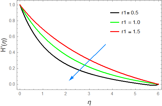
Figure 2 shows how the velocity profile responds to variations in the retardation time constant (r2). Unlike r1, increasing r2 shifts the velocity curves upward, suggesting that the fluid maintains its motion over a greater distance from the wall. This behavior reflects that fluids with higher r2 resist immediate deformation, as their internal structure reacts more slowly to applied stresses. Consequently, the momentum boundary layer thickens, producing fuller and more extended velocity profiles. The impact of the Grashof number (G1) on the velocity gradient is depicted in Figure 3. Higher G1 values strengthen buoyancy forces, enhancing fluid motion across the boundary layer. This trend demonstrates the typical free-convection effect: as thermal buoyancy increases, the fluid accelerates upward, generating a more energetic velocity profile. Physically, greater density variations from temperature differences (higher G1) produce stronger upward forces, increasing the fluid’s momentum.
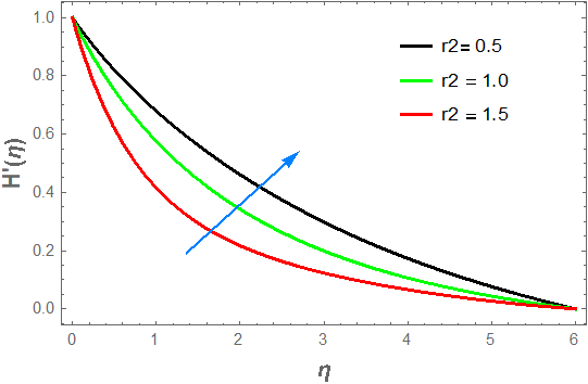
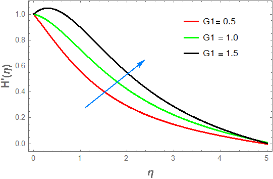
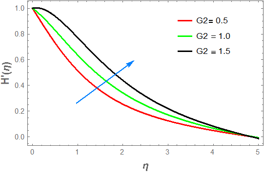
Figure 4 presents the influence of the buoyancy ratio (G2) on the velocity profile. The curves rise with increasing G2, indicating that combined buoyancy effects enhance fluid motion within the boundary layer. This occurs because solutal buoyancy reinforces the existing thermal buoyancy, providing additional lifting force. A higher G2 physically represents stronger concentration-driven density differences, which boost the fluid’s upward movement.
Finally, Figure 5 shows how the velocity profile changes with the Rayleigh number (G3). As G3 increases, the velocity grows gradually, reflecting stronger convection in the flow. Larger Rayleigh numbers indicate that buoyant forces dominate over viscous resistance, demonstrating the direct relationship between thermal-driven density variations and fluid acceleration. Physically, higher G3 values correspond to more pronounced temperature-induced buoyancy effects that propel the fluid more vigorously.
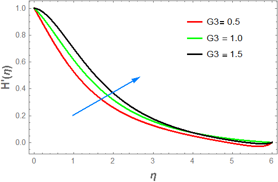
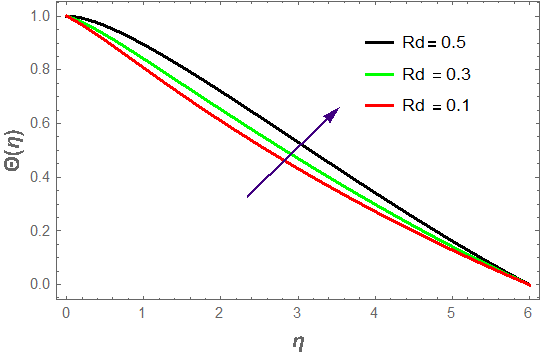
Figure 6 illustrates how the temperature profile responds to changes in the radiation parameter (Rd). As Rd increases, the temperature rises noticeably, highlighting the significant role of radiative heat transfer in enhancing thermal energy within the boundary layer. This trend indicates that higher radiative effects inject additional heat into the fluid, raising its overall temperature. Physically, a larger radiation parameter means that the fluid absorbs and re-emits thermal radiation more efficiently, intensifying heat transfer.
The effect of the thermal relaxation parameter (L1) on temperature is shown in Figure 7. With increasing L1, the temperature decreases, suggesting that thermal relaxation reduces heat buildup within the boundary layer. A higher thermal relaxation indicates that the fluid responds more slowly to temperature changes, limiting the rate of energy transfer. Physically, this delayed response lowers the effective heat conduction, as the fluid takes longer to adapt to imposed thermal gradients.
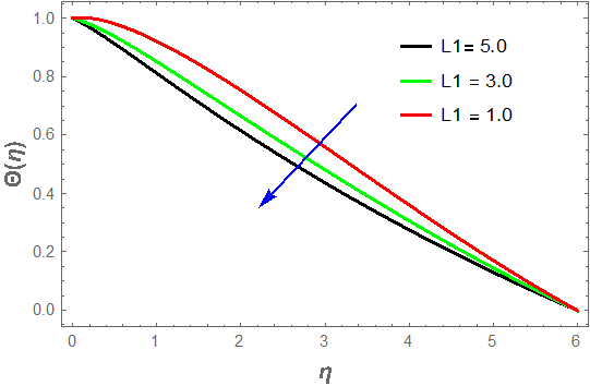
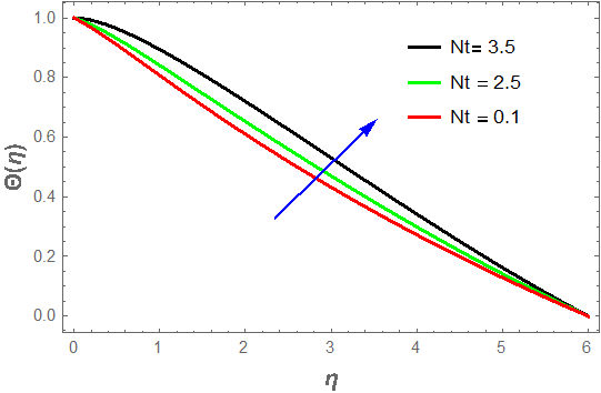
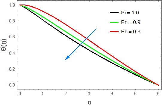
Figure 8 demonstrates the influence of the thermophoresis parameter (Nt) on the temperature profile. As Nt grows, the temperature rises, indicating that thermophoretic motion enhances heat accumulation in the boundary layer. This occurs because nanoparticles move from hotter regions toward cooler areas, transporting thermal energy into the surrounding fluid and enriching the temperature distribution. In physical terms, a larger thermophoresis parameter reflects stronger particle migration driven by temperature gradients. The impact of the Prandtl number (Pr) is presented in Figure 9. Higher Pr values lead to a sharper decline in the temperature profile, indicating that fluids with larger Prandtl numbers dissipate heat more efficiently and form a thinner thermal boundary layer. This behavior arises because momentum diffusion dominates over thermal diffusion in high-Pr fluids. Physically, a higher Pr corresponds to a fluid with relatively low thermal conductivity compared to its viscosity.
Finally, Figure 10 shows the effect of the Dufour number (B) on the temperature distribution. As B increases, the temperature rises significantly, reflecting enhanced heat transfer due to concentration gradients. This illustrates the Dufour (diffusion-thermo) effect, where mass diffusion contributes directly to thermal energy transport. Physically, a larger Dufour number indicates that solutal effects supply additional heat to the fluid, boosting the temperature beyond what is achieved by conduction and convection alone.
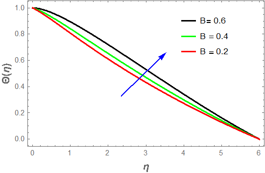
Figure 11 illustrates the effect of the thermophoresis parameter (Nt) on the concentration profile. As Nt increases, the concentration rises throughout the boundary layer, indicating that thermophoretic forces drive nanoparticles away from the heated surface, enhancing species accumulation deeper into the fluid. This upward trend highlights the influence of temperature-driven particle motion on the concentration field. Physically, a larger Nt corresponds to stronger nanoparticle migration due to temperature differences, causing the concentration to decrease more gradually with increasing eta as particles carry species from hot to cooler regions. The influence of the chemical reaction parameter (Cr) is shown in Figure 12. With higher Cr values, the concentration decreases sharply, reflecting the depletion of species caused by intensified chemical activity within the fluid. This behavior represents the accelerated consumption or decay of diffusing species due to faster reactions. Physically, a larger chemical reaction parameter signifies a more vigorous reaction rate, which reduces species levels more rapidly, particularly away from the wall, leading to a thinner concentration boundary layer.
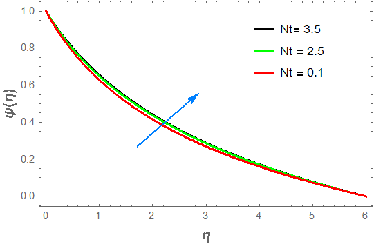
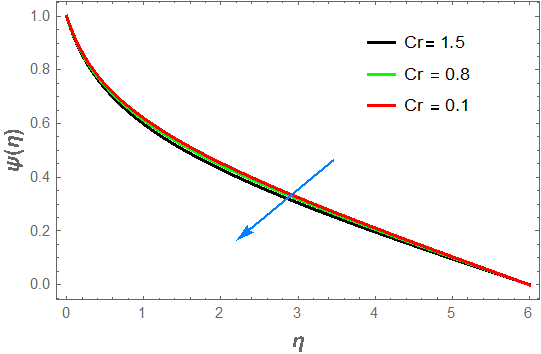
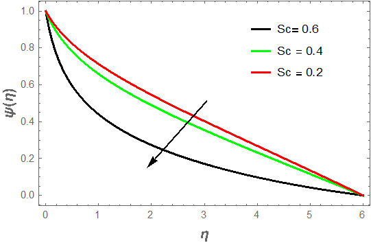
Figure 13 presents the effect of the Schmidt number (Sc) on the concentration distribution. As Sc increases, the concentration drops more steeply, indicating that species diffusion weakens while momentum diffusion dominates. This trend is typical of fluids with high Schmidt numbers, where mass diffusivity is low and the concentration adjusts rapidly near the surface. Physically, a higher Sc reflects lower molecular diffusivity of the species in the fluid.
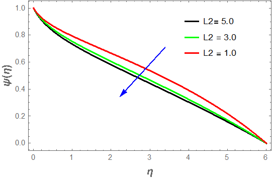
Finally, Figure 14 shows the impact of the concentration relaxation parameter (L2) on the concentration profile. As L2 rises, the concentration decreases steadily, suggesting that a longer relaxation time slows the diffusion-driven spread of species within the boundary layer. This downward shift indicates the delayed response of the concentration field to imposed gradients. Physically, a larger L2 means that species do not respond immediately to spatial changes, leading to a slower development of the concentration profile.
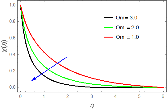
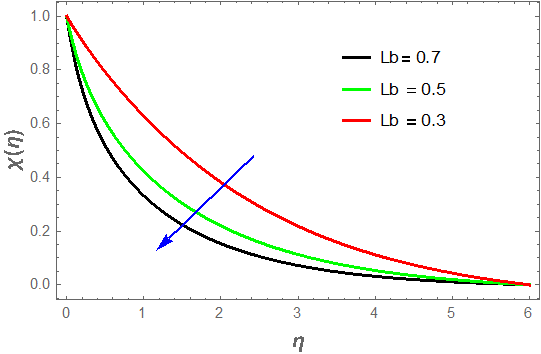
Figures 15-17 show the influence of the Peclet number (Pe), microorganism concentration difference (Om), and bio-convection Lewis number (Lb) on the distribution of microorganisms. In all cases, increasing these parameters reduces microorganism accumulation within the boundary layer, indicating that stronger advection, larger concentration gradients, and higher bio-convective resistance limit microbial dispersion. Physically, a higher Peclet number means convective transport dominates over diffusion, causing microorganisms to spread more rapidly and lowering their concentration near the surface. An increase in the concentration difference (Om) drives microbes away from regions of higher concentration, enhancing depletion. Similarly, a larger bio-convection Lewis number (Lb) decreases the effectiveness of microbial diffusion relative to bio-convective transport, resulting in a thinner, more confined microorganism concentration layer.

This study analyzed the flow and transport characteristics of Oldroyd-B nanofluid under the CCDD framework, incorporating mixed convection, Arrhenius-type chemical reactions, and motile microorganisms. The nonlinear governing equations were solved numerically using the CCM, capturing the non-Fourier and non-Fickian behavior of the model with stable and accurate results. Momentum transfer was found to be strongly affected by relaxation and retardation times, with increased relaxation slowing the fluid and higher retardation enhancing velocity. Buoyancy-driven parameters, including Grashof, buoyancy ratio, and Rayleigh numbers, enhanced fluid motion and expanded the momentum boundary layer.
Thermal and mass transport exhibited distinct responses to various physical factors. Radiation, thermophoresis, and the Dufour effect elevated temperature, while higher Prandtl numbers and thermal relaxation limited heat diffusion. Species concentration increased with thermophoresis and Dufour effects but decreased due to chemical reaction, concentration relaxation, and higher Schmidt numbers, which restrict diffusion or accelerate species depletion. Overall, resistive effects (high Prandtl or Schmidt numbers, and relaxation) compressed the boundary layer, whereas driving mechanisms (buoyancy, radiation, thermophoresis, Dufour) expanded it. The CCDD framework highlighted the delayed thermal and concentration responses compared to classical models, revealing complex but predictable interactions among nanoparticles, chemical reactions, and mixed convection that can be tuned to control heat and mass transport effectively.
The authors praise Ladoke Akintola University of Technology’s Department of Pure and Applied Mathematics for its excellent research facilities.
According to the authors, they have no conflicting interests.