
The development of flexible probability models remains an important topic in distribution theory and applied statistics. In many practical settings, including reliability, survival analysis, actuarial science, engineering, and finance, observed data exhibit right-skewness, varying tail behaviour, and hazard shapes that may be increasing, decreasing, bathtub-shaped, or unimodal. Classical distributions such as the exponential and Weibull models are often attractive because of their simplicity, but they may be too restrictive for these more complex patterns [1, 2]. This motivates the continuing search for distributional extensions that preserve tractability while allowing richer shapes.
A common strategy for constructing such models is to embed a baseline distribution inside a generator family. The resulting “G-family” approach has produced many useful classes, including the beta-G family [3], the Kumaraswamy-G family [4], the gamma-G family [5], and the Topp-Leone-G family [6]. By introducing additional shape mechanisms, these constructions often improve flexibility in the density and hazard functions while retaining interpretable links with established baseline models.
The Topp-Leone generator has been combined with several baseline distributions in the literature. Related examples include extensions based on Weibull, Fréchet, inverse Pareto, and other lifetime models [7– 15]. In parallel, the New Weighted-Weibull (NWW) distribution provides a useful Weibull-type baseline with additional shape control [16]. Bringing these two ideas together leads naturally to the Topp-Leone New Weighted-Weibull (TLNWW) construction studied in this paper.
The main purpose of this work is not merely to introduce the TLNWW form, but also to clarify its mathematical structure and practical interpretation. In particular, after substitution, the distribution depends on the composite rate parameter \(k=2\alpha(1+\beta^\theta)\) and can be written in exponentiated Weibull form. This observation is important because it shows that inference is most naturally carried out through the identifiable parameter set \((k,\theta,\lambda)\), while the original \((\alpha,\beta)\) representation should be viewed as a redundant reparameterization. Recognizing this point strengthens the theoretical development, avoids overstatement of novelty, and makes the inferential section more coherent.
Accordingly, the specific objectives of the study are to derive the distributional properties of the TLNWW model, establish its reduced composite-parameter representation, obtain estimation equations under maximum likelihood, examine finite-sample behaviour through Monte Carlo simulation, and assess empirical performance using two real datasets. The paper therefore contributes a more careful and transparent treatment of the TLNWW model: it preserves the original construction, clarifies its relationship to existing distributions, and evaluates its practical usefulness in comparison with related competitors.
The TL-G family CDF and PDF, with generator parameter \(\lambda>0\) and baseline CDF \(G(x)\), are given by \[F(x;\lambda)=\left[1-\bar{G}^{\,2}(x)\right]^\lambda,\] \[f(x;\lambda)=2\lambda g(x)\bar{G}(x)\left[1-\bar{G}^{\,2}(x)\right]^{\lambda-1},\] where \(\bar{G}(x)=1-G(x)\).
The PDF and CDF of the NWW distribution [16] with parameters \(\alpha,\theta,\beta>0\) are \[g(x;\alpha,\theta,\beta)=\alpha\theta x^{\theta-1}\left(1+\beta^\theta\right)e^{-\alpha(1+\beta^\theta)x^\theta}, \qquad x>0,\] \[G(x;\alpha,\theta,\beta)=1-e^{-\alpha(1+\beta^\theta)x^\theta}.\]
Applying the Topp-Leone generator to the NWW baseline yields the CDF and PDF of the TLNWW distribution: \[\label{eq1} F_{TLNWW}(x)=\left[1-e^{-2\alpha\left(1+\beta^\theta\right)x^\theta}\right]^\lambda, \qquad x>0,\ \alpha,\theta,\beta,\lambda>0, \tag{1}\] \[\label{eq2} f_{TLNWW}(x)=2\lambda\alpha\left(1+\beta^\theta\right)\theta x^{\theta-1}e^{-2\alpha\left(1+\beta^\theta\right)x^\theta}\left[1-e^{-2\alpha\left(1+\beta^\theta\right)x^\theta}\right]^{\lambda-1}. \tag{2}\]
If \[k=2\alpha\left(1+\beta^\theta\right),\] then Eqs. (1)–(2) become \[F_{TLNWW}(x)=\left[1-e^{-kx^\theta}\right]^\lambda,\] \[f_{TLNWW}(x)=\lambda k\theta x^{\theta-1}e^{-kx^\theta}\left[1-e^{-kx^\theta}\right]^{\lambda-1}.\] This reduced representation shows that the fitted distribution depends on \(\alpha\) and \(\beta\) only through the composite rate \(k\).
Proof of a valid PDF. Using \(\int_{0}^{\infty}f_{TLNWW}(x)\,dx=1\) and setting \(u=1-e^{-kx^\theta}\), we have \[du=k\theta x^{\theta-1}e^{-kx^\theta}dx,\] with limits \(x:0\to\infty\) corresponding to \(u:0\to1\). Therefore, \[\begin{aligned} \int_{0}^{\infty}f_{TLNWW}(x)dx &=\int_{0}^{\infty}\lambda k\theta x^{\theta-1}e^{-kx^\theta}\left[1-e^{-kx^\theta}\right]^{\lambda-1}dx \notag\\ &=\lambda\int_{0}^{1}u^{\lambda-1}du =\lambda\left[\frac{u^\lambda}{\lambda}\right]_{0}^{1}=1. \end{aligned} \tag{3}\]
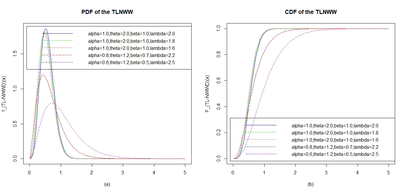
Figure 1 shows the TLNWW distribution for selected parameter values: panel (a) presents the PDF and panel (b) presents the CDF
The survival function of the TLNWW distribution is \[S_{TLNWW}(x)=1-F_{TLNWW}(x)=1-\left[1-e^{-kx^\theta}\right]^{\lambda}. \tag{4}\]
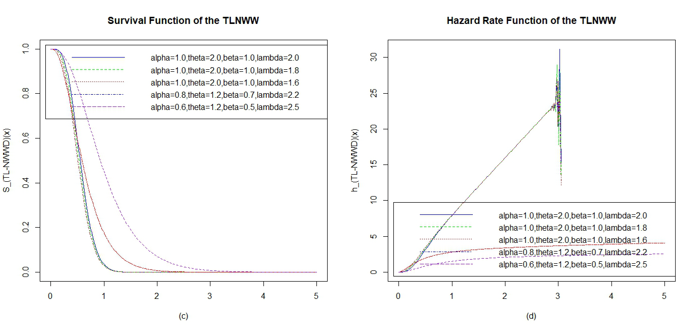
The hazard rate function is \[\begin{aligned} HF_{TLNWW}(x) &=\dfrac{f_{TLNWW}(x)}{S_{TLNWW}(x)} \notag\\ &=\dfrac{\lambda k\theta x^{\theta-1}e^{-kx^\theta}\left[1-e^{-kx^\theta}\right]^{\lambda-1}}{1-\left[1-e^{-kx^\theta}\right]^\lambda}, \end{aligned} \tag{5}\] and the corresponding cumulative hazard function is \[CH_{TLNWW}(x)=-\ln\left\{S_{TLNWW}(x)\right\} =-\ln\left\{1-\left[1-e^{-kx^\theta}\right]^{\lambda}\right\}. \tag{6}\] The form of the hazard function shows that the model can accommodate several shapes according to the values of \(\theta\) and \(\lambda\).
Figure 2 shows the TLNWW distribution for selected parameter values: panel (c) presents the survival function and panel (d) presents the hazard function.
Proposition 1. The TLNWW distribution is algebraically equivalent to an exponentiated Weibull distribution under the reparameterization \(a=\lambda\), \(b=k=2\alpha(1+\beta^\theta)\), and Weibull shape parameter \(\theta\). In the special case \(\lambda=1\), the model reduces to the Weibull distribution with CDF \(F(x)=1-e^{-kx^\theta}\). This observation is important for interpretation: the construction is naturally motivated through the Topp-Leone generator applied to the NWW baseline, but the identifiable fitted distribution is most appropriately expressed through the parameter set \((k,\theta,\lambda)\).
The moment generating function (MGF) of the TLNWW distribution is defined by \[M_X(t)=E\left[e^{tX}\right]=\int_{0}^{\infty}e^{tx}f_{TLNWW}(x)dx. \tag{7}\] For the present model, a convenient representation is obtained through its power-series expansion around \(t=0\), \[M_X(t)=\sum_{r=0}^{\infty}\frac{t^r}{r!}E\left[X^r\right], \tag{8}\] whenever the series converges in a neighbourhood of the origin.
For \(r>-\theta\), the \(r^{th}\) raw moment is \[\begin{aligned} \label{eq13} E\left[X^{r}\right] &=\int_{0}^{\infty}x^{r}f_{TLNWW}(x)dx=\int_{0}^{\infty}x^{r}\lambda k\theta x^{\theta-1}e^{-kx^\theta}\left[1-e^{-kx^\theta}\right]^{\lambda-1}dx. \end{aligned} \tag{9}\]
Let \(y=kx^\theta\). Then \(x=(y/k)^{1/\theta}\) and \(dy=k\theta x^{\theta-1}dx\), so that \[E\left[X^{r}\right]=\lambda k^{-r/\theta}\int_{0}^{\infty}y^{r/\theta}e^{-y}\left(1-e^{-y}\right)^{\lambda-1}dy.\]
Using the binomial expansion \[\left(1-e^{-y}\right)^{\lambda-1}=\sum_{j=0}^{\infty}(-1)^j\begin{pmatrix}\lambda-1\\ j\end{pmatrix}e^{-jy},\] we obtain \[\label{eq16} E\left[X^{r}\right] =\lambda k^{-r/\theta}\Gamma\left(\frac{r}{\theta}+1\right) \sum_{j=0}^{\infty}(-1)^j\begin{pmatrix}\lambda-1\\ j\end{pmatrix}\frac{1}{(j+1)^{\frac{r}{\theta}+1}}. \tag{10}\]
Hence the first four raw moments are obtained from Eq. (10) by taking \(r=1,2,3,4\), respectively. In particular, \[E[X]=\lambda k^{-1/\theta}\Gamma\left(\frac{1}{\theta}+1\right)\sum_{j=0}^{\infty}(-1)^j\begin{pmatrix}\lambda-1\\ j\end{pmatrix}\frac{1}{(j+1)^{\frac{1}{\theta}+1}},\] \[E[X^2]=\lambda k^{-2/\theta}\Gamma\left(\frac{2}{\theta}+1\right)\sum_{j=0}^{\infty}(-1)^j\begin{pmatrix}\lambda-1\\ j\end{pmatrix}\frac{1}{(j+1)^{\frac{2}{\theta}+1}},\] \[E[X^3]=\lambda k^{-3/\theta}\Gamma\left(\frac{3}{\theta}+1\right)\sum_{j=0}^{\infty}(-1)^j\begin{pmatrix}\lambda-1\\ j\end{pmatrix}\frac{1}{(j+1)^{\frac{3}{\theta}+1}},\] and \[E[X^4]=\lambda k^{-4/\theta}\Gamma\left(\frac{4}{\theta}+1\right)\sum_{j=0}^{\infty}(-1)^j\begin{pmatrix}\lambda-1\\ j\end{pmatrix}\frac{1}{(j+1)^{\frac{4}{\theta}+1}}.\]
The variance and central moments follow in the usual way: \[\sigma^2=E[X^2]-\mu^2,\] \[\mu_3=E[X^3]-3\mu E[X^2]+2\mu^3,\] \[\mu_4=E[X^4]-4\mu E[X^3]+6\mu^2E[X^2]-3\mu^4.\] Accordingly, the skewness and kurtosis coefficients are \[\gamma_1=\frac{\mu_3}{\sigma^3}, \qquad \gamma_2=\frac{\mu_4}{\sigma^4}.\]
The quantile function of the TLNWW distribution is defined by \[Q_{TLNWW}(u)=F^{-1}(u).\]
Let \[u=\left[1-e^{-2\alpha\left(1+\beta^{\theta}\right)x^{\theta}}\right]^\lambda.\] Since \(k=2\alpha\left(1+\beta^{\theta}\right)\), this becomes \[u=\left[1-e^{-kx^{\theta}}\right]^\lambda,\] and hence \[Q_{TLNWW}(u)=\left[-\dfrac{1}{2\alpha\left(1+\beta^{\theta}\right)}\ln\left(1-u^{\frac{1}{\lambda}}\right)\right]^{\frac{1}{\theta}}.\]
The same expression can be written as: \[\label{eq17} { Q_{TLNWW}(u)=\left[-\dfrac{1}{k}ln\left(1-u^{\frac{1}{\lambda}}\right)\right]^{\frac{1}{\theta}}} . \tag{11}\]
Eq. (11) is the quantile function of the TLNWW distribution. It can be used to compute the first quartile, median, and third quartile by taking \(u=0.25\), \(0.50\), and \(0.75\), respectively, after substituting the fitted parameter values.
The \(i^{th}\) order statistic \(X_{(1)},X_{(2)},\ldots,X_{(n)}\) from a sample of size \(n\) from the TLNWW distribution has density \[\label{eq18} f_{X_{(i)}}(x)=\dfrac{n!}{(i-1)!(n-i)!}\left[F_{TLNWW}(x)\right]^{i-1}\left[1-F_{TLNWW}(x)\right]^{n-i}f_{TLNWW}(x), \tag{12}\] where \(f_{TLNWW}(x)\) and \(F_{TLNWW}(x)\) are the PDF and CDF of the proposed distribution. Substituting Eqs. (1) and (2) into Eq. (12) gives
\[f_{X_{(i)}}(x)=\dfrac{n!}{(i-1)!(n-i)!}\lambda k\theta x^{\theta-1}e^{-kx^\theta}\left[1-e^{-kx^\theta}\right]^{\lambda i-1}\left\{1-\left[1-e^{-kx^\theta}\right]^\lambda\right\}^{n-i}. \tag{13}\]
For the minimum order statistic \((i=1)\), \[f_{X_{(1)}}(x)=n\lambda k\theta x^{\theta-1}e^{-kx^\theta}\left[1-e^{-kx^\theta}\right]^{\lambda-1}\left\{1-\left[1-e^{-kx^\theta}\right]^\lambda\right\}^{n-1}. \tag{14}\]
For the maximum order statistic \((i=n)\), \[f_{X_{(n)}}(x)=n\lambda k\theta x^{\theta-1}e^{-kx^\theta}\left[1-e^{-kx^\theta}\right]^{\lambda n-1}. \tag{15}\]
Because the TLNWW distribution depends on \(\alpha\) and \(\beta\) only through the composite rate \(k=2\alpha(1+\beta^\theta)\), likelihood-based inference is most naturally carried out for the identifiable parameter vector \((k,\theta,\lambda)\). For a random sample \(x_1,x_2,\ldots,x_n\), the likelihood function is \[L_{TLNWW}(x;k,\theta,\lambda)=\prod_{i=1}^{n}f_{TLNWW}(x_i). \tag{16}\]
Hence the log-likelihood function is \[\ell(k,\theta,\lambda)=n\ln\lambda+n\ln k+n\ln\theta+(\theta-1)\sum_{i=1}^{n}\ln x_i-k\sum_{i=1}^{n}x_i^\theta+(\lambda-1)\sum_{i=1}^{n}\ln\left(1-e^{-kx_i^\theta}\right). \tag{17}\]
Differentiating with respect to \(k\), \(\theta\), and \(\lambda\) gives the score equations \[\dfrac{\partial \ell}{\partial k}=\dfrac{n}{k}-\sum_{i=1}^{n}x_i^\theta+(\lambda-1)\sum_{i=1}^{n}\dfrac{x_i^\theta e^{-kx_i^\theta}}{1-e^{-kx_i^\theta}}, \tag{18}\] \[\label{eq30} \dfrac{\partial \ell}{\partial \theta} =\dfrac{n}{\theta}+\sum_{i=1}^{n}\ln x_i-k\sum_{i=1}^{n}x_i^\theta\ln x_i+(\lambda-1)k\sum_{i=1}^{n}\dfrac{x_i^\theta \ln x_i\, e^{-kx_i^\theta}}{1-e^{-kx_i^\theta}}, \tag{19}\] and \[\label{eq31} \dfrac{\partial \ell}{\partial \lambda} =\dfrac{n}{\lambda}+\sum_{i=1}^{n}\ln\left(1-e^{-kx_i^\theta}\right). \tag{20}\]
From Eq. (20), the profile update for \(\lambda\) is \[\hat{\lambda}=-\dfrac{n}{\sum_{i=1}^{n}\ln\left(1-e^{-k x_i^\theta}\right)},\] which is positive because \(\ln(1-e^{-k x_i^\theta})<0\) for all \(x_i>0\). The remaining equations do not admit closed-form solutions and were solved numerically with a Newton–Raphson routine implemented in R under positivity constraints. Multiple starting values were used to reduce sensitivity to local behaviour. For consistency with the original notation, the empirical tables later in the paper retain the four-parameter display \((\alpha,\theta,\beta,\lambda)\); however, inferential interpretation should be based on the implied composite rate \(k=2\alpha(1+\beta^\theta)\).
Based on the theoretical results presented earlier, this section reports a simulation study together with applications to two real datasets. The aim is to assess finite-sample estimation behaviour and to compare the empirical adequacy of the TLNWW model with closely related competitors. Because the fitted distribution is identified through \((k,\theta,\lambda)\), the discussion below emphasizes the implied composite-rate representation even when the original four-parameter notation is retained in the tables.
A Monte Carlo simulation with 5000 replications was conducted for sample sizes \(n=25,50,75,100,200,500,\) and \(1000\) under four representative settings corresponding to \((k,\theta,\lambda)=(10,2,1)\), \((8,1,2)\), \((4,2,3)\), and \((12,1,4)\). These settings arise from the original parameter combinations \(\ (\alpha=1.0, \theta=2, \beta=2.0, \lambda=1.0), \quad (\alpha=2.0, \theta=1.0, \beta=1.0, \lambda=2.0), \quad (\alpha=1.0, \theta=2.0, \beta=1.0, \lambda=3.0)\) and \(\ (\alpha=2.0, \theta=1.0, \beta=2.0, \lambda=4.0).\) The following summary measures were recorded: average bias (ABias), mean absolute error (MAE), mean squared error (MSE), root mean squared error (RMSE), coverage probability (CP), average width (AW), and mean absolute percentage error (MAPE). The results are displayed in Table 1.
| n | Setting | ABias | MAE | MSE | RMSE | CP | AW | MAPE |
|---|---|---|---|---|---|---|---|---|
| 25 | \(S_1\) | -0.4942 | 0.5007 | 0.3345 | 0.5783 | 0.6242 | 1.1775 | 0.5077 |
| 50 | -0.4992 | 0.5002 | 0.2912 | 0.5396 | 0.3218 | 0.8036 | 0.5002 | |
| 75 | -0.4973 | 0.4973 | 0.2751 | 0.5245 | 0.1512 | 0.6534 | 0.4973 | |
| 100 | -0.4999 | 0.4999 | 0.2709 | 0.5205 | 0.0696 | 0.5692 | 0.4999 | |
| 200 | -0.4963 | 0.4963 | 0.2568 | 0.5067 | 0.0016 | 0.3999 | 0.4963 | |
| 500 | -0.4993 | 0.4993 | 0.2535 | 0.5035 | 0.0000 | 0.2526 | 0.4993 | |
| 1000 | -0.5006 | 0.5006 | 0.2527 | 0.5027 | 0.0000 | 0.1718 | 0.5006 | |
| 25 | \(S_2\) | -0.0075 | 0.7344 | 0.8749 | 0.9354 | 0.9476 | 3.6670 | 0.3672 |
| 50 | 0.0010 | 0.5077 | 0.4131 | 0.6428 | 0.9472 | 2.5199 | 0.2539 | |
| 75 | 0.0075 | 0.4051 | 0.2626 | 0.5124 | 0.9486 | 2.0087 | 0.2026 | |
| 100 | 0.0041 | 0.3445 | 0.1881 | 0.4336 | 0.9546 | 1.7000 | 0.1722 | |
| 200 | -0.0041 | 0.2495 | 0.0986 | 0.3141 | 0.9514 | 1.2312 | 0.1248 | |
| 500 | 0.0015 | 0.1603 | 0.0402 | 0.2005 | 0.9500 | 0.7861 | 0.0816 | |
| 1000 | 0.0003 | 0.1132 | 0.0203 | 0.1426 | 0.9508 | 0.5589 | 0.0566 | |
| 25 | \(S_3\) | -1.4992 | 1.4997 | 2.4620 | 1.5691 | 0.0924 | 1.8153 | 0.4999 |
| 50 | -1.4968 | 1.4968 | 2.3409 | 1.5300 | 0.0040 | 1.2418 | 0.4989 | |
| 75 | -1.5035 | 1.5035 | 2.3281 | 1.5258 | 0.0000 | 1.0178 | 0.5012 | |
| 100 | -1.5036 | 1.5036 | 2.3105 | 1.5200 | 0.0000 | 0.8734 | 0.5012 | |
| 200 | -1.5009 | 1.5009 | 2.2772 | 1.5090 | 0.0000 | 0.6128 | 0.5003 | |
| 500 | -1.4995 | 1.4995 | 2.2586 | 1.5029 | 0.0000 | 0.3917 | 0.4998 | |
| 1000 | -1.5012 | 1.5012 | 2.2586 | 1.5029 | 0.0000 | 0.2803 | 0.5003 | |
| 25 | \(S_4\) | 0.0064 | 0.4721 | 0.3534 | 0.5945 | 0.9532 | 2.3306 | 0.1180 |
| 50 | 0.0075 | 0.3309 | 0.1744 | 0.4173 | 0.9454 | 1.6370 | 0.0827 | |
| 75 | -0.0064 | 0.2667 | 0.1120 | 0.3347 | 0.9508 | 1.3118 | 0.0667 | |
| 100 | 0.0028 | 0.2282 | 0.0820 | 0.2864 | 0.9490 | 1.1227 | 0.0571 | |
| 200 | 0.0002 | 0.1641 | 0.0425 | 0.2061 | 0.9490 | 0.8079 | 0.0410 | |
| 500 | -0.0013 | 0.1023 | 0.0165 | 0.1286 | 0.9482 | 0.5040 | 0.0256 | |
| 1000 | 0.0012 | 0.0721 | 0.0081 | 0.0902 | 0.9504 | 0.3537 | 0.0180 |
Table 1 indicates mixed finite-sample performance. In Settings \(S_2\) and \(S_4\), the bias, RMSE, and MAPE generally decrease as \(n\) increases, and the coverage probability remains close to the nominal level. By contrast, Settings \(S_1\) and especially \(S_3\) show persistent bias and severe undercoverage, even for large samples. These results suggest that likelihood-based inference for the TLNWW model can be stable in some regions of the parameter space but numerically challenging in others; consequently, the simulation evidence should be interpreted as scenario-dependent rather than uniformly favourable.
The proposed distribution, together with other competing distributions, is applied to two real datasets to evaluate flexibility and empirical fit. Model selection criteria, including the Akaike Information Criterion (AIC), Consistent Akaike Information Criterion (CAIC), Bayesian Information Criterion (BIC), and Hannan–Quinn Information Criterion (HQIC), are employed. In addition, parameter estimates, standard errors, Anderson–Darling (AD), Kolmogorov–Smirnov (KS), and the associated \(p\)-value are reported. The Shapiro–Wilk statistic (\(W\)) is retained in the tables as a descriptive benchmark, but model comparison is based primarily on likelihood-based criteria and distributional fit summaries.
Dataset 1: Comprises 100 observations on the breaking stress of carbon fibres, obtained from [17]. This dataset is used to evaluate the performance of the proposed model. The results, presented in Tables 2–4 and Figure 3, include the descriptive statistics, measures of goodness-of-fit, model selection criteria, and graphical assessments through the PDF, and Empirical Cumulative Distribution Function (ECDF) plots.
| Min | 1st Qu | Median | 3rd Qu | Mean | Var | Max | Skewness | Kurtosis |
|---|---|---|---|---|---|---|---|---|
| 0.390 | 1.840 | 2.700 | 3.220 | 2.621 | 1.025 | 5.560 | 0.368 | 3.105 |
| Model | \(\ \hat{\alpha}\) | \(\ \hat{\theta}\) | \(\ \hat{\beta}\) | \(\ \hat{\lambda}\) | W | AD | KS |
|---|---|---|---|---|---|---|---|
| TLNWW | 0.0438 | 2.4075 | 0.3163 | 1.3180 | 0.0704 | 0.4132 | 0.0645 |
| (0.0983) | (0.5923) | (5.0536) | (0.5854) | [0.7994] | |||
| TLWW | 0.0205 | 2.3628 | 1.1656 | 1.3619 | 0.0720 | 0.4169 | 0.0660 |
| (0.0261) | (0.5969) | (1.3361) | (0.6237) | [0.7778] | |||
| TLW | 0.0180 | 1.2821 | 2.3593 | 1.3684 | 0.0722 | 0.4172 | 0.0661 |
| (0.0208) | (1.3357) | (0.6196) | (0.6512) | [0.7753] | |||
| WD | 0.0133 | 1.6725 | 2.2919 | 1.4436 | 0.0750 | 0.4247 | 0.0677 |
| (0.0104) | (1.3240) | (0.6028) | (0.6970) | [0.7495] |
| Model | -2Logl | AIC | BIC | CAIC | HQIC |
|---|---|---|---|---|---|
| TLNWW | 141.332 | 290.664 | 301.085 | 291.085 | 294.882 |
| TLWW | 141.335 | 290.670 | 301.091 | 291.091 | 294.888 |
| TLW | 141.336 | 290.671 | 301.092 | 291.092 | 294.889 |
| WD | 141.352 | 290.705 | 301.125 | 291.126 | 294.922 |
Figure 3 shows the fitted distributions: panel (e) presents the PDF plots and panel (f) presents the CDF plots.
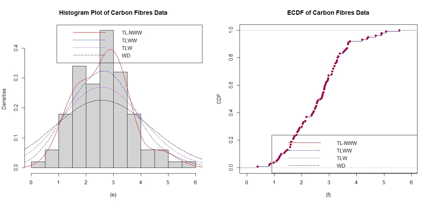
Tables 2–4 report the descriptive statistics, parameter estimates, and model selection criteria for Dataset 1. The data exhibit mild positive skewness (0.368) and moderate kurtosis (3.105), indicating a slightly asymmetric but not highly heavy-tailed distribution. The competing models fit this dataset very similarly: TLNWW attains the smallest information criteria, but the numerical differences from TLWW and TLW are slight. The goodness-of-fit measures and the fitted curves in Figure 3 therefore support the more cautious conclusion that TLNWW is competitive for Dataset 1 rather than decisively superior.
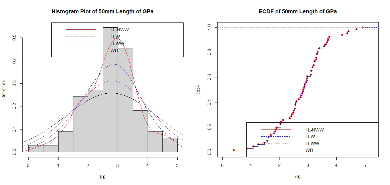
Dataset 2: Consists of measurements on 50 mm fibre length (GPa), originally reported by [18] and later utilized by [19]. This dataset is employed to further evaluate the performance of the proposed models. The results, summarized in Tables 5–7 and Figure 4, include the descriptive statistics, goodness-of-fit measures, model selection criteria, and graphical assessments through the PDF and ECDF plots.
| Min | 1st Qu | Median | 3rd Qu | Mean | Var | Max | Skewness | Kurtosis |
|---|---|---|---|---|---|---|---|---|
| 0.390 | 1.840 | 2.178 | 2.835 | 3.277 | 2.760 | 4.900 | 0.795 | 3.220 |
| Model | \(\ \hat{\alpha}\) | \(\ \hat{\theta}\) | \(\ \hat{\beta}\) | \(\ \hat{\lambda}\) | W | AD | KS |
|---|---|---|---|---|---|---|---|
| TLNWW | 0.0082 | 0.0261 | 3.6006 | 0.9080 | 0.0897 | 0.5159 | 0.0847 |
| (0.0056) | (6.1176) | (0.4605) | (0.2182) | [0.7305] | |||
| TLWW | 0.0091 | 0.0041 | 3.5320 | 0.9386 | 0.0910 | 0.5197 | 0.0853 |
| (0.0067) | (1.1626) | (0.4888) | (0.2398) | [0.7231] | |||
| TLW | 0.0090 | 0.0842 | 3.5400 | 0.9339 | 0.0908 | 0.5193 | 0.0853 |
| (0.0066) | (5.0395) | (0.5145) | (0.2470) | [0.7227] | |||
| WD | 0.0172 | 0.0322 | 3.1230 | 1.1543 | 0.1021 | 0.5635 | 0.0900 |
| (0.0183) | (9.2753) | (0.6913) | (0.4461) | [0.6584] |
| Model | -2Logl | AIC | BIC | CAIC | HQIC |
|---|---|---|---|---|---|
| TLNWW | 85.990 | 179.980 | 188.739 | 180.636 | 183.441 |
| TLWW | 86.014 | 180.028 | 188.786 | 180.683 | 183.489 |
| TLW | 86.101 | 180.021 | 188.780 | 180.677 | 183.482 |
| WD | 86.282 | 180.564 | 189.323 | 181.220 | 184.025 |
Tables 5–7 show that Dataset 2 is more clearly right-skewed than Dataset 1, and the TLNWW model again yields the smallest information criteria among the models considered. In this case the advantage is still modest, but it is somewhat more consistent across the reported criteria and fit summaries than in Dataset 1. The fitted PDF and CDF curves in Figure 4 are compatible with this ranking and indicate that the proposed model captures the upper-tail behaviour reasonably well.
The numerical results suggest that the TLNWW model is a useful and competitive distribution for positively skewed lifetime data, but they do not support an unqualified claim of uniform superiority. For Dataset 1, the improvement in information criteria over TLWW and TLW is very small, so the principal conclusion is one of comparable fit with a slight advantage to TLNWW. For Dataset 2, the advantage of TLNWW is somewhat clearer, although the competing models remain close. The graphical fits in Figures 3–4 are consistent with these findings.
An important outcome of the revised analysis is the clarification that the model is most appropriately interpreted through the composite rate parameter \(k=2\alpha(1+\beta^\theta)\). This reduced representation resolves the identifiability concern raised by the algebraic form of the distribution and aligns the theoretical development with the estimation procedure. The simulation study further shows that numerical performance depends on the parameter setting: some scenarios display the expected reduction in estimation error with increasing sample size, whereas others exhibit persistent bias and undercoverage. This pattern highlights the need for careful initialization, constraint handling, and diagnostic checking when fitting the model in practice.
Overall, the manuscript supports the view that the TLNWW construction provides a tractable exponentiated Weibull-type representation with flexible hazard behaviour and competitive empirical performance. Its value lies in the combination of generator-based motivation, transparent reparameterization, and practical applicability, rather than in claiming a wholly distinct identifiable four-parameter family.
This study examined the Topp–Leone New Weighted-Weibull distribution from both a constructive and inferential perspective. The main theoretical result is that the model obtained from the Topp–Leone generator applied to the NWW baseline can be written in the reduced form \[F(x)=\left[1-e^{-kx^\theta}\right]^\lambda,\] with \(k=2\alpha(1+\beta^\theta)\). This representation clarifies the model’s link with the exponentiated Weibull family and identifies the parameter set through which inference should be interpreted.
Within this framework, explicit expressions were obtained for the density, survival function, hazard function, quantile function, order statistics, and moments, and maximum likelihood estimation was formulated for the identifiable parameters. The simulation study showed that estimation performs well in some parameter settings but may be unstable in others, especially with respect to interval coverage. The real-data applications demonstrated that the TLNWW model provides competitive fits and can outperform related alternatives by small margins, particularly for right-skewed engineering data.
Consequently, the TLNWW model should be regarded as a useful and carefully reparameterized lifetime distribution with practical modelling value. Future work may focus on alternative estimation strategies, broader comparative studies, and residual-based diagnostics to better understand the parameter regions in which numerical fitting is most reliable.
Sokenu, M. R. contributed to the mathematical development and literature synthesis. Badmus, N. I. formulated the study, implemented the R code, and conducted the numerical analyses. Oyeyemi, S. T. contributed to the literature review, interpretation of results, and proofreading of the manuscript
The authors declare no conflict of interest.
The data used in this study were extracted from [17– 19].
No external funding was received for this research.
The authors thank the reviewers and colleagues whose comments helped improve the clarity and rigor of the manuscript
The authors declare no conflict of interest.