
In high-frequency financial markets, transaction durations provide essential information on market microstructure, liquidity formation, and risk transmission mechanisms [1]. Duration data are strictly positive and typically exhibit pronounced right skewness, heavy tails, and temporal dependence, with clustering behavior analogous to volatility clustering in asset returns [2]. These characteristics pose substantial challenges for classical duration models.
The Autoregressive Conditional Duration (ACD) model introduced by [3] addresses such dependence by decomposing observed durations into a conditional mean component and a stochastic innovation. Within this framework, the choice of the innovation distribution is critical, as it governs the shape of the conditional intensity function and the model’s capacity to capture persistence and tail behavior [4]. Although several extensions have been proposed, including the Weibull, Log-Weibull, and Generalized Gamma ACD models [5, 6], most of these specifications impose monotonic intensity structures and therefore failure to accommodate empirically observed non-monotonic patterns such as unimodal or bathtub-shaped intensities [7].
An additional challenge in ACD modeling concerns the treatment of intraday seasonality. Many existing studies adopt two-step pre-filtering procedures to remove calendar effects prior to model estimation [8]. This strategy implicitly assumes independence between deterministic intraday patterns and stochastic duration dynamics. In high-frequency financial markets, however, these components are often interrelated, and separating them may result in biased parameter estimates and distorted statistical inference [9].
Recent developments in distribution theory indicate that secant-based generators provide a flexible and analytically tractable framework for modeling heavy-tailed data with complex conditional intensity shape. In particular, the Secant-\(G\) family proposed by [10] allows for rich non-monotonic intensity structures. Despite its flexibility, this class of distributions has not yet been explored within the ACD modeling framework.
Motivated by these considerations, this study proposes the Secant-Weibull Autoregressive Conditional Duration model with calendar effects (SW-ACD-X). The model employs the Secant-Weibull distribution as a flexible innovation specification and incorporates calendar effects directly into the conditional mean equation. This joint modeling strategy captures intraday seasonality and stochastic duration dynamics simultaneously, thereby reducing the biases associated with conventional two-step approaches.
The following section establishes an ACD framework that incorporates calendar effects and presents the Secant-Weibull distribution as a flexible innovation specification. Parameter estimation is performed using a dual approach: Frequentist Maximum Likelihood Estimation (MLE) and Bayesian inference via RStan. The proposed framework is subsequently verified through empirical analysis and Monte Carlo simulation studies.
To describe the time interval between two consecutive events occurring at times \(t_i\) and \(t_{i-1}\), the duration is defined as \(x_i = t_i – t_{i-1}.\) Following the seminal Autoregressive Conditional Duration (ACD) framework of [3], each observed duration \(x_i\) is decomposed into a predictable conditional mean component \(\psi_i\) and a stochastic innovation \(\epsilon_i\), such that \[\begin{equation} x_i = \psi_i \epsilon_i, \qquad \epsilon_i \sim \text{i.i.d. } g(\epsilon; \boldsymbol{\theta}), \label{eq:1} \end{equation} \tag{1}\] where \(g(\cdot)\) is the probability density function of the innovation term, and \(E[\epsilon_i] = 1\).
A primary limitation of traditional ACD specifications is the need for external pre-filtering to remove diurnal seasonality. To address this issue, the SW–ACD–X(1,1) model incorporates calendar effects directly into the conditional mean by including a vector of indicator variables \(Z_{i-1,1}\) within the recursion as follows: \[\begin{equation} \psi_i = \omega + \alpha_1 x_{i-1} + \beta_1 \psi_{i-1} + \gamma_1 Z_{i-1,1} \label{eq:2}. \end{equation} \tag{2}\]
By estimating the calendar-effect coefficients \(\boldsymbol{\gamma_1}\) jointly with the Autoregressive parameters \(\alpha_1\) and \(\beta_1\), the proposed model captures the interaction between deterministic intraday patterns and stochastic duration clustering.
The Secant-Weibull (SW) distribution is a new and flexible two-parameter model developed from the Secant-G family [10]. It is obtained by applying a trigonometric secant transformation to the CDF of the classical Weibull distribution. This structure gives the SW distribution strong adaptability, enabling it to capture features often observed in financial duration data, such as skewness, heavy tails (leptokurtosis), and non-monotonic conditional intensity patterns. A major advantage of the SW distribution is its simplicity: with only two parameters, it can represent all six well-known intensity shapes including hump-shaped and bathtub-shaped that are difficult to capture with the standard Weibull or more complex models like the Log Weibull distribution. The SW distribution is a good option for modelling improvements in ACD models because of the balance between flexibility and symmetry. We use the CDF of Weibull distribution as the baseline,given by \[G(x) = 1 – e^{-(x/\lambda)^k}, \quad x \geq 0,\; \lambda > 0,\; k > 0 .\]
By applying the transformation defined in the preceding equation, we derive the Secant-Weibull distribution,with the CDF given by \[\begin{equation} F(x) = \sec\left( \frac{\pi}{3} \left( 1 – e^{-(x/\lambda)^k} \right) \right) – 1 . \label{eq:3} \end{equation} \tag{3}\]
The PDF of SW distribution is given by \[\begin{equation} f(x) = \frac{\pi k}{3 \lambda} \left( \frac{x}{\lambda} \right)^{k-1} e^{-(x/\lambda)^k} \sec \left[ \frac{\pi}{3} \left( 1 – e^{-(x/\lambda)^k} \right) \right] \tan \left[ \frac{\pi}{3} \left( 1 – e^{-(x/\lambda)^k} \right) \right] . \label{eq:4} \end{equation} \tag{4}\]
The conditional intensity function is given by
\[h(x) = \frac{f(x)}{1 – F(x)} .\]
Substituting the PDF \(f(x)\) and duration function \(1 – F(x)\), we get the following conditional intensity function: \[h(x) = \frac{ \frac{\pi k}{3\lambda} \left(\frac{x}{\lambda}\right)^{k-1} e^{-(x/\lambda)^k} \cdot \sec\left(\frac{\pi}{3}\left(1 – e^{-(x/\lambda)^k}\right)\right) \tan\left(\frac{\pi}{3}\left(1 – e^{-(x/\lambda)^k}\right)\right) }{ 2 – \sec\left(\frac{\pi}{3}\left(1 – e^{-(x/\lambda)^k}\right)\right) }.\]
The secant and tangent transformations in the Secant-Weibull distribution allow for non-monotonic, heavy-tailed shapes of conditional intensity. This flexibility improves model fit for financial durations that often display overdispersion, extreme events, and volatility clustering.
Quantile Function. The Quantile function is essential for Monte Carlo simulations and is derived by inverting the CDF: \[\begin{equation} Q(u) = \lambda \left[ -\ln \left( 1 – \frac{3}{\pi} \operatorname{arcsec} (u+1) \right) \right]^{1/k}, \label{Eq:6} \end{equation} \tag{5}\] where \(u\in (0,1)\).This allows for the direct generation of Secant-Weibull random variables.
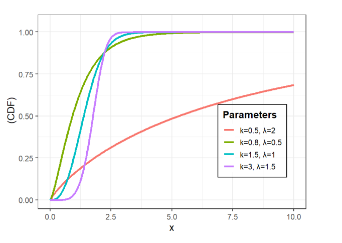
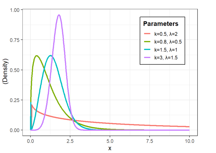
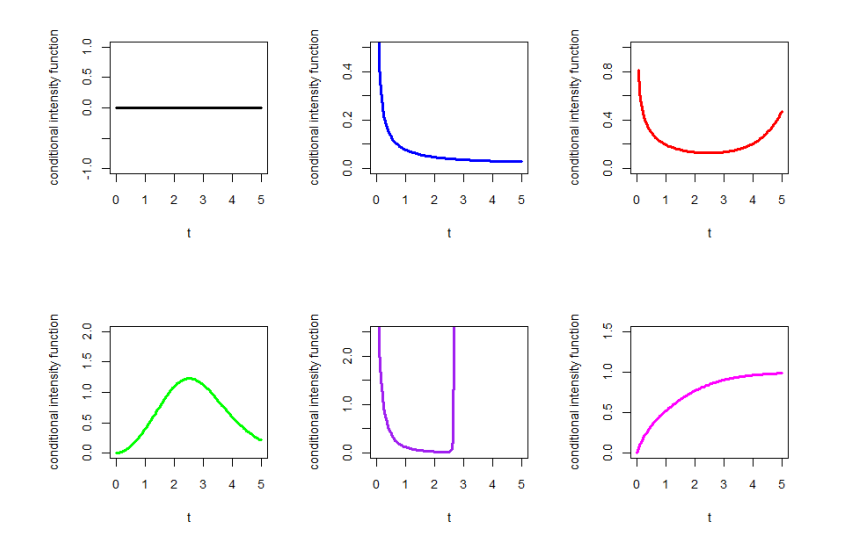
In this subsection, we present the different shapes of the CDF and PDF shown in Figures 1 and 2 respectively. Figure 3 illustrate six distinct forms of the conditional intensity function: constant, decreasing, bathtub, unimodal, modified bathtub, and increasing intensity.
To evaluate the persistence, information flow, and risk dynamics of high-frequency durations, we derive three key properties of the SW distribution: Rényi Entropy, the expected Remaining Wait Time , and Order Statistics.
Rényi entropy measures the uncertainty or “disorder” in the timing of market events. It generalizes Shannon entropy and is particularly useful for understanding information flow in limit order books. For the SW distribution, Rényi entropy of order \(v\) (\(v > 0\), \(v \neq 1\)) for a random variable \(X\) with PDF \(f(x)\) is defined as follows: \[\begin{equation} \text{RE}_X(v) = \frac{1}{1-v} \log \left[ \int_0^\infty f^v(x)\, dx \right]. \end{equation} \tag{6}\]
For the SW distribution with scale PDF is (4).
Substituting \(f(x)\) into the integral gives
\[\begin{equation} \int_0^\infty f^v(x) \, dx = \left( \frac{\pi k}{3 \lambda} \right)^v \int_0^\infty \left(\frac{x}{\lambda}\right)^{v(k-1)} e^{-v(x/\lambda)^k} \left[ \sec\left( \frac{\pi}{3} (1 – e^{-(x/\lambda)^k}) \right) \tan\left( \frac{\pi}{3} (1 – e^{-(x/\lambda)^k}) \right) \right]^v dx. \end{equation} \tag{7}\]
Expanding the trigonometric term via a series and applying the binomial theorem,we get \[\begin{equation} \left[ \sec\left( \frac{\pi}{3} (1 – e^{-(x/\lambda)^k}) \right) \tan\left( \frac{\pi}{3} (1 – e^{-(x/\lambda)^k}) \right) \right]^v \\ = \sum_{m=0}^\infty \sum_{j=0}^\infty a_m(v) \binom{2m+v}{j} (-1)^j \left( \frac{\pi}{3} \right)^{2m+v} e^{-j(x/\lambda)^k}, \end{equation} \tag{8}\] where the coefficients \(a_m(v)\) are determined from derivatives of \([\sec(s)\tan(s)]^v\) at \(s=0\).
Performing the change of variable \(y = (x/\lambda)^k\) so that \(x = \lambda y^{1/k}\) and \(dx = \frac{\lambda}{k} y^{1/k-1} dy\), the integral becomes a gamma function:
\[\begin{equation} \int_0^\infty \left(\frac{x}{\lambda}\right)^{v(k-1)} e^{-(v+j)(x/\lambda)^k} dx = \lambda k \, \Gamma\left( \frac{v(k-1)+1}{k} \right) (v+j)^{-(v(k-1)+1)/k}. \end{equation} \tag{9}\]
Substituting back, the Rényi entropy is
\[\begin{equation} RE_X(v) = \frac{1}{1-v} \log \Bigg[ \Gamma\left( \frac{v(k-1)+1}{k} \right) \sum_{m=0}^\infty \sum_{j=0}^\infty a_m(v) \binom{2m+v}{j} (-1)^j \left( \frac{\pi}{3} \right)^{2m+v} \lambda k (v+j)^{-(v(k-1)+1)/k} \Bigg]. \end{equation} \tag{10}\]
In financial contexts, higher entropy indicates a high degree of ”market noise” or randomness in trade arrivals. Conversely, a decrease in entropy suggests a more structured arrival process, typically associated with periods of informed trading or institutional ”meta-order” execution where durations become more predictable (clustering).
The expected Remaining Wait Time is crucial for algorithmic execution. It represents the expected time until the next trade occurs, given that \(t\) seconds have already elapsed since the last event. Within the framework of the SW distribution, this function is derived as: \[m(t) = E[X – t \mid X > t] = \frac{1}{S(t)} \int_{t}^{\infty} S(x) \, dx.\]
For the Secant-Weibull specification with duration function \(S(x) = 2 – \sec\left[ \frac{\pi}{3}(1 – e^{-(x/\lambda)^k}) \right]\), this definition leads to the expression: \[m(t) = \frac{\displaystyle \int_{t}^{\infty} \left\{ 2 – \sec\left[ \frac{\pi}{3}\left(1 – e^{-(x/\lambda)^k}\right) \right] \right\} dx}{\, 2 – \sec\left[ \frac{\pi}{3}\left(1 – e^{-(t/\lambda)^k}\right) \right] \,}.\]
For a liquidity provider, \(m(t)\) measures the “Expected Remaining Wait Time.” Unlike the standard Weibull model, which imposes monotonic waiting times, the SW distribution allows for a bathtub-shaped trajectory . This captures a realistic market scenario where, if a long period passes without a trade, the expected time until the next trade may actually increase as the market becomes illiquid or “stale.”
To quantify the behavior of the fastest trades (HFT activity) and the longest gaps (liquidity dry-ups), we utilize order statistics. Let \(X_{(i)}\) denote the \(i\)-th order statistic in a sample of \(n\) durations. The probability density function (PDF) of \(X_{(i)}\) is given by:
\[\begin{equation} f_{i:n}(x) = \frac{n!}{(i-1)!(n-i)!} f(x) [F(x)]^{i-1} [1-F(x)]^{n-i}, \label{eq:14} \end{equation} \tag{11}\] where \(f(x)\) and \(F(x)\) are the PDF and CDF of the underlying duration distribution. Substituting specific form \(f(x)\) and \(F(x)\) into Eq. (11) yields the distribution of extreme duration events.
\[\begin{aligned} f_{i:n}(x) =& \frac{n!}{(i-1)!(n-i)!} \cdot \left[\frac{\pi k}{3\lambda}\left(\frac{x}{\lambda}\right)^{k-1} e^{-(x/\lambda)^k}\right] \times \sec\left[\frac{\pi}{3}\left(1-e^{-(x/\lambda)^k}\right)\right] \tan\left[\frac{\pi}{3}\left(1-e^{-(x/\lambda)^k}\right)\right] \\ &\times \left[\sec\left[\frac{\pi}{3}\left(1-e^{-(x/\lambda)^k}\right)\right] – 1\right]^{i-1} \times \left[2 – \sec\left[\frac{\pi}{3}\left(1-e^{-(x/\lambda)^k}\right)\right]\right]^{n-i}. \end{aligned}\] In the context of high-frequency trading, the extreme values of trade durations provide critical insights into market microstructure. The first order statistic \(X_{(1)}\) represents the “Maximum Market Speed” in a sample, while the \(n\)-th statistic \(X_{(n)}\) captures the “Maximum Liquidity Gap.” This formulation is essential for stress-testing trading algorithms against “flash-clumps” (many trades in milliseconds) or “flash-crashes” (total cessation of trading).
The first Order Statistic :the minimum duration \(X_{(1)}\) (\(i = 1\)), the PDF simplifies to \[\begin{aligned} f_{X_{(1)}}(x) &= n \; f(x) \; [1 – F(x)]^{n-1} \\ &= n \cdot \left[ \frac{\pi k}{3\lambda} \left(\frac{x}{\lambda}\right)^{\!k-1} e^{-(x/\lambda)^k} \right] \times \sec\!\left[\frac{\pi}{3}\left(1 – e^{-(x/\lambda)^k}\right)\right] \tan\!\left[\frac{\pi}{3}\left(1 – e^{-(x/\lambda)^k}\right)\right] \\ &\quad \times \left[ 2 – \sec\!\left[\frac{\pi}{3}\left(1 – e^{-(x/\lambda)^k}\right)\right] \right]^{n-1}. \end{aligned}\]
The n-the Order Statistic :the maximum duration \(X_{(n)}\) (\(i = n\)), the PDF simplifies to \[\begin{aligned} f_{X_{(n)}}(x) &= n \; f(x) \; [F(x)]^{n-1} \\ &= n \cdot \left[ \frac{\pi k}{3\lambda} \left(\frac{x}{\lambda}\right)^{\!k-1} e^{-(x/\lambda)^k} \right] \times \sec\!\left[\frac{\pi}{3}\left(1 – e^{-(x/\lambda)^k}\right)\right] \tan\!\left[\frac{\pi}{3}\left(1 – e^{-(x/\lambda)^k}\right)\right] \\ &\quad \times \left[ \sec\!\left[\frac{\pi}{3}\left(1 – e^{-(x/\lambda)^k}\right)\right] – 1 \right]^{n-1}. \end{aligned}\]
These expressions are mathematically valid only for \(x\) satisfying the domain condition of the secant function, that is \(0 \leq (\pi/3)\left(1 – e^{-(x/\lambda)^k}\right) < (\pi/2).\)
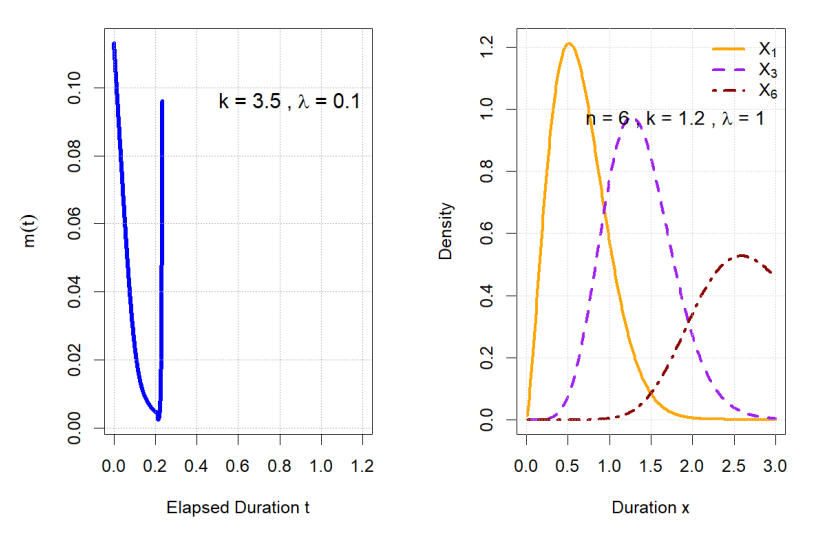
Figure 4 illustrates these properties: the right plot (Expected Remaining Wait Time) displays the bathtub shape essential for realistic liquidity modeling, while the left plot (Order Statistics) shows the distribution of extremes, which is crucial for algorithmic trading risk analysis.
The SW-ACD-X model characterizes durations as \(x_i = \psi_i \epsilon_i\), where \(\epsilon_i\) is a stochastic innovation and \(\psi_i\) is the conditional mean. To account for deterministic intraday patterns simultaneously with stochastic clustering, we specify the conditional mean as Eq. (2). where \(Z_{i-1,1}\) represents exogenous calendar variables (time-of-day dummies). The standard SW-ACD model is recovered as a special case of this formulation when \(\gamma_l = 0\) for all \(l\). To ensure model identifiability and maintain the interpretation of \(\psi_i\) as the actual conditional expected duration, we impose the unit-mean constraint \(E[\epsilon_i] = 1\).
The \(r\)-th raw moment of the SW distribution is essential for defining the structural properties of the innovation term. Substituting the PDF from Eq. (4) into the moment definition \(\mathbb{E}[\epsilon^r] = \int_0^\infty x^r f(x) dx\), we obtain
\[\begin{equation} \mu'_r = \mathbb{E}[\epsilon^r] = \frac{\pi k}{3\lambda} \int_0^\infty x^r \left( \frac{x}{\lambda} \right)^{k-1} e^{-(x/\lambda)^k} \sec\left[ \frac{\pi}{3} \left( 1 – e^{-(x/\lambda)^k} \right) \right] \tan\left[ \frac{\pi}{3} \left( 1 – e^{-(x/\lambda)^k} \right) \right] dx . \end{equation} \tag{12}\]
To evaluate this integral analytically, we utilize the power series expansion of the circular trigonometric product \(\sec(z)\tan(z)\) via Euler numbers \(E_{2m+1}\). The \(r\)-th moment is derived as \[\begin{equation} \mu'_r = \lambda^r \Gamma \left( 1 + \frac{r}{k} \right) \sum_{m=0}^{\infty} \frac{E_{2m+1}}{(2m+1)!} \left( \frac{\pi}{3} \right)^{2m+2} \sum_{j=0}^{2m+1} \binom{2m+1}{j} \frac{(-1)^j}{(j+1)^{1+r/k}}, \label{eq:19} \end{equation} \tag{13}\] where \(E_{2m+1}\) are the Euler numbers. To satisfy the ACD requirement \(\mathbb{E}[\epsilon_i] = 1\), we set \(r = 1\) and define the scaling factor \(\Lambda_k\) such that \[\begin{equation} \Lambda_k = \Gamma \left( 1 + \frac{1}{k} \right) \sum_{m=0}^{\infty} \frac{E_{2m+1}}{(2m+1)!} \left( \frac{\pi}{3} \right)^{2m+2} \sum_{j=0}^{2m+1} \binom{2m+1}{j} \frac{(-1)^j}{(j+1)^{1+1/k}} .\label{eq:20} \end{equation} \tag{14}\]
By imposing the identification constraint \(\lambda = 1/\Lambda_k\), the scale parameter becomes a restricted function of the shape parameter \(k\). This reduces the parameter space by one dimension, preventing numerical redundancy and resolving the structural competition between the intercept \(\omega\) and the scale parameter. This moment property and identification constraint are identical for both the SW–ACD and SW–ACD–X models. For numerical implementation, the infinite series in Eq. (14) is evaluated using a truncation at \(M = 50\) terms, as follows: \[\begin{equation} \Lambda_k \approx \Gamma \left( 1 + \frac{1}{k} \right) \sum_{m=0}^{50} \frac{E_{2m+1}}{(2m+1)!} \left( \frac{\pi}{3} \right)^{2m+2} \sum_{j=0}^{2m+1} \binom{2m+1}{j} \frac{(-1)^j}{(j+1)^{1+1/k}}. \label{eq:21} \end{equation} \tag{15}\]
The truncation error is rigorously controlled by the radius of convergence of the power series (\(|z| < \pi/2\)). Since the argument is \(z = \pi/3\), the ratio \(z/R = 2/3\) ensures a geometric decay of terms, allowing the approximation to reach machine precision (\(< 10^{-16}\)) at \(M=50\). Numerical stability is preserved for the shape parameter range \(0.5 < k < 5\) typically observed in financial durations, as the factorial growth in the denominator effectively offsets the growth of the Euler numbers.
By substituting the identification constraint into the general density, the PDF of the standardized innovations \(\epsilon_i \sim SW(k)\) is expressed as follows: \[\begin{equation} \begin{aligned} g(\epsilon_i; k) = & \frac{\pi k \Lambda_k}{3} (\epsilon_i \Lambda_k)^{k-1} \exp \left[ -(\epsilon_i \Lambda_k)^k \right] \cdot \sec \left[ \frac{\pi}{3} \left( 1 – e^{-(\epsilon_i \Lambda_k)^k} \right) \right] \tan \left[ \frac{\pi}{3} \left( 1 – e^{-(\epsilon_i \Lambda_k)^k} \right) \right], \quad \epsilon_i > 0. \end{aligned} \end{equation} \tag{16}\]
This standardized innovation distribution is common to both the SW–ACD–X and the SW–ACD models.
Given the transformation \(\epsilon_i = x_i/\psi_i\) and the Jacobian \(\left| d\epsilon_i/dx_i \right| = 1/\psi_i\), the conditional PDF of the observed duration \(x_i\) given the filtration \(\mathcal{F}_{i-1}\) is \[\begin{align} \label{eq:23} f(x_i \mid \mathcal{F}_{i-1}; \boldsymbol{\theta}) &= \frac{1}{\psi_i} \cdot g\left(\frac{x_i}{\psi_i}; k\right) \notag\\ &= \frac{\pi k \Lambda_k}{3\psi_i} \left(\frac{x_i \Lambda_k}{\psi_i}\right)^{k-1} \exp\left[-\left(\frac{x_i \Lambda_k}{\psi_i}\right)^k\right] \times \sec\left[\frac{\pi}{3}\left(1 – \exp\left[-\left(\frac{x_i \Lambda_k}{\psi_i}\right)^k\right]\right)\right] \notag\\ &\quad \times \tan\left[\frac{\pi}{3}\left(1 – \exp\left[-\left(\frac{x_i \Lambda_k}{\psi_i}\right)^k\right]\right)\right], \end{align} \tag{17}\] where \(\boldsymbol{\theta} = (\omega, \alpha_1, \beta_1, k)^\top\) is the parameter vector, and \(\Lambda_k\) is computed from \(k\) via Eq. (13).
The SW–ACD–X model yields an analytical Quantile function that integrates the Autoregressive dynamics and the seasonal parameters \(\gamma_l\). For a probability level \(\tau \in (0,1)\), the \(\tau\)-Quantile is given by: \[\begin{equation} Q_{x_i}(\tau | \mathcal{F}_{i-1}) = \frac{\psi_i}{\Lambda_k} \left[ -\ln \left( 1 – \frac{3}{\pi} \operatorname{arcsec}(\tau + 1) \right) \right]^{1/k}. \label{eq:24} \end{equation} \tag{18}\]
where \(\psi_i\) is defined as in Eq. (2). this analytical formulation facilitates both Monte Carlo simulation and direct likelihood evaluation for parameter estimation, while nesting the SW–ACD model as a special case where \(\gamma_l = 0\) for all \(l\).
The conditional intensity function \(h(x_i \mid \mathcal{F}_{i-1})\) provides crucial insights into market dynamics by quantifying the instantaneous probability of a trade occurring given the time elapsed since the last transaction and past market information. The formula of conditional intensity function is: \[\begin{equation} h(x_i \mid \mathcal{F}_{i-1}) = \frac{\frac{\pi k \Lambda_k}{3 \psi_i} (x_i \Lambda_k / \psi_i)^{k-1} \exp \left[ -(x_i \Lambda_k / \psi_i)^k \right] \sec \left( \frac{\pi}{3} \left[ 1 – e^{-(x_i \Lambda_k / \psi_i)^k} \right] \right) \tan \left( \frac{\pi}{3} \left[ 1 – e^{-(x_i \Lambda_k / \psi_i)^k} \right] \right)}{2 – \sec \left( \frac{\pi}{3} \left[ 1 – e^{-(x_i \Lambda_k / \psi_i)^k} \right] \right)}. \end{equation} \tag{19}\]
The conditional intensity function \(h(x_i \mid \mathcal{F}_{i-1})\) characterizes the instantaneous probability of an event, dynamically scaled by the conditional mean \(\psi_i\) to reflect varying market speeds. Its unique trigonometric specification allows the model to capture complex, non-monotonic conditional intensity such as consolidation periods and momentum building while the standardization \(\Lambda_k\) ensures that the innovation process remains scale-invariant with a unit mean.
This section details the estimation procedures for the Secant-Weibull distribution and the subsequent ACD frameworks, utilizing both Frequentist and Bayesian paradigms. Frequentist estimation is conducted via (MLE), while Bayesian inference is implemented using (HMC) with the (NUTS). The numerical properties of the SW distribution allow for flexible and complex shapes in the conditional intensity of durations across both frameworks.
The parameter vector of the SW distribution, \(\boldsymbol{\theta} = (\lambda, k)^\top\), is estimated using the (MLE) method. By maximizing the likelihood function associated with the observed data, the frequentist estimates of the parameters \(\lambda\) and \(k\) are obtained.
Let \(\mathbf{x} = (x_1, x_2, \ldots, x_n)\) denote a random sample of \(n\) independent and identically distributed (i.i.d.) observations drawn from the SW distribution. The likelihood function \(L(\boldsymbol{\theta}\mid \mathbf{x})\)is defined as the joint probability density of the sample and is given by \[\begin{equation} \begin{aligned} L(\boldsymbol{\theta}\mid \mathbf{x}) = \prod_{i=1}^n \Biggl[ & \frac{\pi}{3} \cdot \frac{k}{\lambda} \left( \frac{x_i}{\lambda} \right)^{k – 1} e^{-(x_i / \lambda)^k} \cdot \sec\left( \frac{\pi}{3} \left( 1 – e^{-(x_i / \lambda)^k} \right) \right) \cdot \tan\left( \frac{\pi}{3} \left( 1 – e^{-(x_i / \lambda)^k} \right) \right) \Biggr]. \end{aligned} \label{eq:26} \end{equation} \tag{20}\]
The log-likelihood function is obtained by taking the natural logarithm of the likelihood function, as follows:
\[\begin{align*} \ell(\boldsymbol{\theta} \mid \mathbf{x}) &= \sum_{i=1}^n \ln \Biggl[ \frac{\pi}{3} \cdot \frac{k}{\lambda} \left( \frac{x_i}{\lambda} \right)^{k – 1} e^{-(x_i / \lambda)^k} \cdot \sec\left( \frac{\pi}{3} \left(1 – e^{-(x_i / \lambda)^k} \right) \right) \cdot \tan\left( \frac{\pi}{3} \left(1 – e^{-(x_i / \lambda)^k} \right) \right) \Biggr]. \end{align*}\]
When accounting for temporal dependencies and intraday seasonality, the observed durations \(x_i\) are no longer i.i.d. Instead, they are modeled as \(x_i = \psi_i \epsilon_i\), where the stochastic innovations follow a Secant-Weibull distribution, denoted as \(\epsilon_i \sim \text{SW}(k)\). The parameter vector to be estimated is defined as \(\boldsymbol{\theta} = (\omega, \alpha_1, \beta_1, \gamma_1,k)^\top\).
While the specification of the conditional mean \(\psi_i\) differs between the standard SW–ACD and the SW–ACD–X (the latter incorporating calendar effects \(\gamma_l\)), both models share the same conditional density structure. We estimate the parameters by maximizing the conditional log-likelihood. Given the information set \(\mathcal{F}_{i-1}\), the density of \(x_i\) is determined by the innovation distribution, and the conditional likelihood function is \[\begin{equation*} \begin{aligned} L(\boldsymbol{\theta}\mid\mathbf{x}) &= \prod_{i=1}^{n} f(x_i \mid \mathcal{F}_{i-1}; \boldsymbol{\theta}) \\ &= \prod_{i=1}^{n} \left[ \frac{\pi k \Lambda_k}{3 \psi_i} \left(\frac{x_i \Lambda_k}{\psi_i}\right)^{k-1} \exp\left[-\left(\frac{x_i \Lambda_k}{\psi_i}\right)^k\right] \right. \times \sec\left[\frac{\pi}{3}\left(1 – \exp\left[-\left(\frac{x_i \Lambda_k}{\psi_i}\right)^k\right]\right)\right] \\ &\quad \left. \times \tan\left[\frac{\pi}{3}\left(1 – \exp\left[-\left(\frac{x_i \Lambda_k}{\psi_i}\right)^k\right]\right)\right] \right]. \end{aligned} \end{equation*}\]
Taking natural logarithms, the conditional log-likelihood function \(\ell(\theta)\) is expressed as \[\begin{equation*} \begin{aligned} \ell(\boldsymbol{\theta} \mid \mathbf{x}) &= \sum_{i=1}^{n} \left( \ln\left(\frac{\pi}{3}\right) + \ln(k) + k \ln(\Lambda_k) – k \ln(\psi_i) + (k-1) \ln(x_i) – \left[ \frac{x_i \Lambda_k}{\psi_i} \right]^k \right. \\ &\quad + \ln\left[ \sec\left( \frac{\pi}{3} \left( 1 – \exp\left[ -\left( \frac{x_i \Lambda_k}{\psi_i} \right)^k \right] \right) \right) \right] \left. + \ln\left[ \tan\left( \frac{\pi}{3} \left( 1 – \exp\left[ -\left( \frac{x_i \Lambda_k}{\psi_i} \right)^k \right] \right) \right) \right] \right). \end{aligned} \end{equation*}\]
The SW–ACD model is nested within this framework and can be estimated by imposing the restriction \(\gamma_l = 0\) for all \(l\).
The maximum likelihood estimates \(\hat{\boldsymbol{\theta}}\) cannot be obtained analytically due to the recursive form of the conditional mean \(\psi_i\) and the nonlinearity of the Secant–Weibull density. Therefore, the log-likelihood must be maximized using iterative numerical methods, such as the BFGS algorithm, to estimate the parameters. To initialize the recursion for \(\psi_i\) at \(i = 1\), the pre-sample values \((x_0, \psi_0)\) and the exogenous variables \(Z_{l,0}\) are set equal to their respective sample means. During maximum likelihood estimation, these initial values are treated as fixed constants rather than parameters to be estimated.
Parameters are regarded as random variables with prior distributions in the Bayesian method. The posterior distributions are obtained by updating these priors with the observed data using the Bayes theorem. Given the data \(\mathbf{x} = (x_1, \dots, x_n)\) for the Secant–Weibull distribution, the joint posterior distribution of the parameters \(\lambda\) and \(k\) is:
\[p(\lambda, k \mid x) \propto p(x \mid \lambda, k) \cdot p(\lambda) \cdot p(k).\]
For the Secant-Weibull parameters, we specify conditionally independent priors: \[k \sim \text{Gamma}(a_1,c_1), \quad p(k) = \frac{c_1^{a_1}}{\Gamma(a_1)} k^{a_1 – 1} e^{-c_1 k}, \quad k>0, a_1>0, c_1>0,\] \[\lambda \sim \text{Gamma}(a_2, c_2), \quad p(\lambda) = \frac{b_2^{a_2}}{\Gamma(a_2)} \lambda^{a_2 – 1} e^{-c_2 \lambda}, \quad \lambda>0, a_2>0, c_2>0,\] with hyperparameters \(a_1, c_1, a_2, c_2 > 0\). The Gamma prior ensures positivity and provides flexibility in representing prior beliefs about the scale and shape parameters.
The joint posterior distribution combining the likelihood from Eq. (18) with the priors is:
\[\begin{aligned} p(\boldsymbol{\theta}\mid \mathbf{x})&\propto \left[ \prod_{i=1}^{n} f(x_i; \lambda, k) \right] \times p(\lambda) \times p(k) \\ &= \left[ \prod_{i=1}^{n} \frac{\pi}{3} \cdot \frac{k}{\lambda} \left(\frac{x_i}{\lambda}\right)^{k-1} e^{-(x_i/\lambda)^k} \times \sec\left(\frac{\pi}{3} \left(1 – e^{-(x_i/\lambda)^k}\right)\right) \cdot \tan\left(\frac{\pi}{3} \left(1 – e^{-(x_i/\lambda)^k}\right)\right) \right] \\ &\quad \times \frac{c_2^{a_2}}{\Gamma(a_2)} \lambda^{a_2 – 1} e^{-c_2 \lambda} \times \frac{c_1^{a_1}}{\Gamma(a_1)} k^{a_1 – 1} e^{-c_1 k}. \end{aligned}\]
Using the NUTS sampler, we estimate the posterior distributions for \(k\) and \(\lambda\) with Gamma priors for both parameters. The model’s performance is assessed through MCMC diagnostics, ensuring that the potential scale reduction factor (\(\hat{R}\)) is close to 1.00 and that the effective sample size is adequate for reliability .
Bayesian inference provides a probabilistic framework for parameter estimation by combining prior information with observed data through Bayes’ theorem [11]. In this framework, prior distributions represent initial beliefs about the parameters, which are updated using the likelihood of the observed durations to obtain the posterior distribution.
To avoid the structural identification redundancy between the scale of the ACD process (\(\omega\)) and the scale parameter of the innovation distribution (\(\lambda\)), the scale parameter is not estimated directly. Instead, it is treated as a deterministic function of the shape parameter \(k\) such that \(\lambda = 1/\Lambda_k\), where \(\Lambda_k\) is the normalizing constant that ensures the unit mean constraint \(E[\epsilon_i] = 1\). Under this identified specification, the parameter vectors are defined as \(\boldsymbol{\theta} = (\omega, \alpha_1, \beta_1, k)^\top\) for the SW–ACD model, and \(\boldsymbol{\theta}_{X} = (\omega, \alpha_1, \beta_1, \gamma_1, k)^\top\) for the SW–ACD–X model that incorporates calendar-effects.
Weakly informative priors are assigned to ensure that the likelihood dominates the posterior inference while maintaining valid parameter domains, as follows:
\[\omega \sim \text{Gamma}(a_3,c_3), \quad p(\omega) = \frac{c_3^{a_3}}{\Gamma(a_3)} \omega^{a_3 – 1} e^{-c_3 \omega}.\]
\[\alpha_1 \sim \text{Beta}(a_4, b_4), \quad p(\alpha_1) = \frac{\Gamma(a_4 + b_4)}{\Gamma(a_4)\Gamma(b_4)} \alpha_1^{a_4-1} (1-\alpha_1)^{b_4-1}.\]
\[\beta_1 \sim \text{Beta}(a_5, b_5), \quad p(\beta_1) = \frac{\Gamma(a_5 + b_5)}{\Gamma(a_5)\Gamma(b_5)} \beta_1^{a_5-1} (1-\beta_1)^{b_5-1}.\]
For the SW-ACD-X model, the calendar-effect coefficients follow Normal priors,as follows:
\[\gamma_l \sim \text{Normal}(a_6,c_6), \quad p(\gamma_l) = \frac{1}{\sqrt{2\pi c_6}} \exp\left[-\frac{(\gamma_l-a_6)^2}{2c_6}\right].\]
The posterior distribution, \(p(\boldsymbol{\theta} \mid \mathbf{x})\), is derived by combining the conditional likelihood of the SW–ACD model with the joint prior distribution via Bayes’ theorem,as follows: \[p(\boldsymbol{\theta} \mid \mathbf{x}) \propto L(\mathbf{x} \mid \boldsymbol{\theta}) \cdot p(\boldsymbol{\theta}).\]
The joint prior \(p(\boldsymbol{\theta})\) is the product of the individual marginal distributions: \[\begin{equation} p(\boldsymbol{\theta}) = p(\omega) \cdot p(\alpha_1) \cdot p(\beta_1) \cdot p(k). \end{equation} \tag{21}\]
For the SW-ACD(1,1) model, the joint posterior distribution is proportional to \[\begin{align} \label{eq:39} p(\boldsymbol{\theta} \mid \mathbf{x}) &\propto \prod_{i=1}^{n} \Bigg[ \frac{\pi k \Lambda_k}{3 \psi_i} \left( \frac{x_i \Lambda_k}{\psi_i} \right)^{k-1} \exp \left[ -\left( \frac{x_i \Lambda_k}{\psi_i} \right)^k \right] \times \sec \left( \frac{\pi}{3} \left[ 1 – \exp \left[ -\left( \frac{x_i \Lambda_k}{\psi_i} \right)^k \right] \right] \right) \notag\\ &\quad \times \tan \left( \frac{\pi}{3} \left[ 1 – \exp \left[ -\left( \frac{x_i \Lambda_k}{\psi_i} \right)^k \right] \right] \right) \Bigg] \times \frac{c_1^{a_1}}{\Gamma(a_1)} k^{a_1 – 1} e^{-c_1 k} \times \frac{c_3^{a_3}}{\Gamma(a_3)} \omega^{a_3 – 1} e^{-c_3 \omega} \notag\\ &\quad \times \frac{\Gamma(a_4 + b_4)}{\Gamma(a_4)\Gamma(b_4)} \alpha_1^{a_4 – 1} (1 – \alpha_1)^{b_4 – 1} \times \frac{\Gamma(a_5 + b_5)}{\Gamma(a_5)\Gamma(b_5)} \beta_1^{a_5 – 1} (1 – \beta_1)^{b_5 – 1}. \end{align} \tag{22}\]
For the SW–ACD–X specification, the posterior additionally incorporates the priors of the calendar-effect parameters,as follows:
\[\begin{aligned} p(\boldsymbol{\theta}_X \mid \mathbf{x}) &\propto L(\mathbf{x}\mid\boldsymbol{\theta}_X) \, p(\omega)\,p(\alpha_1)\,p(\beta_1)\,p(k) \prod_{l=1}^{m} p(\gamma_l), \end{aligned}\] \[\begin{aligned} p(\boldsymbol{\theta}_{\text{X}} \mid \mathbf{x}) &\propto \prod_{i=1}^{n} \left[ \frac{\pi k \Lambda_k}{3 \psi_i} \left(\frac{x_i \Lambda_k}{\psi_i}\right)^{k-1} \exp\left[-\left(\frac{x_i \Lambda_k}{\psi_i}\right)^k\right] \right. \times \sec\left(\frac{\pi}{3}\left[1 – \exp\left[-\left(\frac{x_i \Lambda_k}{\psi_i}\right)^k\right]\right]\right) \\ &\quad \left. \times \tan\left(\frac{\pi}{3}\left[1 – \exp\left[-\left(\frac{x_i \Lambda_k}{\psi_i}\right)^k\right]\right]\right) \right] \times \frac{c_1^{a_1}}{\Gamma(a_1)} k^{a_1-1} e^{-c_1 k} \times \frac{c_3^{a_3}}{\Gamma(a_3)} \omega^{a_3-1} e^{-c_3 \omega} \\ &\quad \times \frac{\Gamma(a_4 + b_4)}{\Gamma(a_4)\Gamma(b_4)} \alpha_1^{a_4-1} (1-\alpha_1)^{b_4-1}\times \frac{\Gamma(a_5 + b_5)}{\Gamma(a_5)\Gamma(b_5)} \beta_1^{a_5-1} (1-\beta_1)^{b_5-1} \\ &\quad \times \prod_{l=1}^{m} \left[ \frac{1}{\sqrt{2\pi c_6}} \exp\left[-\frac{(\gamma_l – a_6)^2}{2c_6}\right] \right]. \end{aligned}\]
Because the posterior involves nonlinear trigonometric functions and recursive conditional means \(\psi_i\), closed-form solutions are not available. Therefore, parameter estimation is performed using Markov Chain Monte Carlo (MCMC) methods. Specifically, this study employs Hamiltonian Monte Carlo (HMC) with the No-U-Turn Sampler (NUTS) implemented in Stan, which efficiently explores the high-dimensional posterior space and provides stable convergence [12].
To assess the empirical performance of the developed SW–ACD–X model, we compare it with four set up competing specifications. To confirm model identifiability, each innovation process has its unit mean (\(E[\epsilon_i] = 1\)) normalized. The following is a definition of the conditional log-likelihood functions for the competing specifications.
Weibull –ACD–X model. The conditional Log-Likelihood of W–ACD–X is given by \[\begin{align} \ell(\theta) &=\sum_{i=1}^{n} \Bigg[ \log \left( \frac{k}{\psi_i} \right) + \log \left( \left( \Gamma\left(1 + \frac{1}{k}\right) \right)^k \right) + \log \left( \left( \frac{x_i}{\psi_i} \right)^{k-1} \right) – \left( \frac{x_i \cdot \Gamma\left(1 + \frac{1}{k}\right)}{\psi_i} \right)^k \Bigg]. \end{align} \tag{23}\]
Gompertz–ACD–X Model. The conditional Log-Likelihood of G–ACD–X is given by \[\begin{equation} \ell(\theta) = n \ln(b) – \sum_{i=1}^{n} \ln(\psi_i) + b \sum_{i=1}^{n} x_i – \sum_{i=1}^{n} \left( \frac{e^{b x_i} – 1}{\psi_i} \right). \end{equation} \tag{24}\]
Lomax–ACD–x model. The conditional log-likelihood of Lomax–ACD–X model is given by \[\begin{equation} \ell(\theta) = n \ln(k) – \sum_{i=1}^{n} \ln\left[ \psi_i(k-1) \right] – (k+1) \sum_{i=1}^{n} \ln\left( 1 + \frac{x_i}{\psi_i(k-1)} \right). \end{equation} \tag{25}\]
log-weibull–ACD–X model. The conditional log-likelihood of LW–ACD–X model is given by \[\begin{align*} \ell(\theta) &= \sum_{i=1}^n \Bigg[ \ln(k) + k \ln\!\left( \Gamma\!\left(1 + \frac{1}{k}\right) \right) + (k – 1)\ln(x_i) – k \ln(\psi_i) – \left( \Gamma\!\left(1 + \frac{1}{k}\right)\frac{x_i}{\psi_i} \right)^{k} \Bigg]. \end{align*}\]
This section outlines the frequentist and Bayesian approaches employed to compare the proposed SW–ACD–X model with other competing specifications. These metrics allow us to determine the optimal model for capturing the complex dynamics of the data.
In the frequentist framework, model comparison balances goodness-of-fit with model complexity. This study employs two widely used information criteria: the Akaike Information Criterion (AIC), defined as \(\text{AIC} = -2\ell(\hat{\boldsymbol{\theta}}) + 2p\), and the Bayesian Information Criterion (BIC), defined as \(\text{BIC} = -2\ell(\hat{\boldsymbol{\theta}}) + p\ln(n)\), where \(\ell(\hat{\boldsymbol{\theta}})\) denotes the maximized log-likelihood, \(p\) is the number of estimated parameters, and \(n\) is the sample size.
Bayesian model comparison focuses on predictive performance and model evidence, relying on the full posterior distribution rather than point estimates. In this study, model evaluation is conducted using the Watanabe–Akaike Information Criterion (WAIC) and Leave-One-Out Cross-Validation (LOOIC), both of which assess out-of-sample predictive accuracy based on posterior inference.
This section assesses the numerical stability, parameter identifiability, and finite-sample performance of the SW distribution and its dynamic expansions, namely the SW–ACD and SW–ACD–X models. We evaluate the robustness of the suggested estimators in both static and dynamic data-generating environments using both Frequentist and Bayesian frameworks.
Monte Carlo simulations are captured for sample sizes \(n \in \{100, 200, \dots, 1000\}\), with \(R = 100\) independent replications for each design. The finite-sample performance of the estimators is assessed using the Average Bias (AB) and the Mean Squared Error (MSE), defined as \[\begin{equation} AB(\theta) = \frac{1}{N} \sum_{i=1}^{N} \left( \hat{\theta}^{(i)} – \theta \right), \end{equation} \tag{26}\] \[\begin{equation} MSE(\theta) = \frac{1}{N} \sum_{i=1}^{N} \left( \hat{\theta}^{(i)} – \theta \right)^2. \end{equation} \tag{27}\]
Recursively, durations are produced used inverse transform method and i.i.d.\(\epsilon_i\) is first extracted from a unit-mean SW distribution . The Quantile function is then applied to uniform random variables \(u\in (0,1)\). Next, the observed durations are formed as \(x_i = \psi_i \epsilon_i\), where \(\psi_i\) is the conditional mean. This process is equivalent to taking a direct sample at each time point \(i\) from the conditional Quantile function of the model.
we use two different statistical methods. To have a thorough understanding of model dependability and parameter uncertainty.
The simulation is structured to assess three levels of model complexity:
Baseline SW Distribution. The parameter vector is \(\boldsymbol{\theta} = (\lambda, k)\). We evaluate the MLE across sample sizes \(n \in \{100, \dots, 1000\}\) with \(R = 100\) independent Monte Carlo replications. The true values are set at \(\lambda = 0.8\) and \(k = 1.2\).
SW–ACD Model. The dynamic parameter vector is \(\boldsymbol{\theta} = (\omega, \alpha_1, \beta_1, k)\). True values are fixed at \(\omega = 0.2, \alpha_1 = 0.15, \beta_1 = 0.7\), and \(k = 1.2\). This setup assesses the model’s ability to capture Autoregressive clustering.
SW–ACD–X Model. The vector expands to \(\boldsymbol{\theta} = (\omega, \alpha_1, \beta_1, \gamma_1, k)\), where \(\gamma_1 = 0.02\) represents a deterministic calendar effect. This design tests the simultaneous estimation of stochastic and exogenous components.
In the Bayesian framework, posterior recovery is assessed using a
synthetic dataset of size \(n = 1000\).
Inference is conducted via the HMC–NUTS sampler in Stan
using four parallel chains and 2,000 iterations (including 1,000 warm up
draws). To ensure reproducibility, hyperparameters are set to weakly
informative values: the intercept follows \(\omega \sim \text{Gamma}(1, 10)\),while the
scale and shape parameters follow \(\lambda
\sim \text{Gamma}(2,2)\) and \(k \sim
\text{Gamma}(2,2)\), respectively. For the Autoregressive
parameters, we specify jointly truncated Beta priors over the
stationarity simplex to strictly satisfy \(\alpha_1 + \beta_1 < 1\), with \(\alpha_1 \sim \text{Beta}(1.5, 15)\) and
\(\beta_1 \sim \text{Beta}(15, 1.5)\).
The calendar effect coefficient is assigned a \(\gamma_1 \sim \text{Normal}(0, 0.25)\)
prior.
This setup ensures that the likelihood dominates the posterior while keeping parameters within their theoretically valid domains. Convergence is monitored via trace plots and the Gelman-Rubin diagnostic, ensuring all parameters achieve \(\hat{R} < 1.01\).
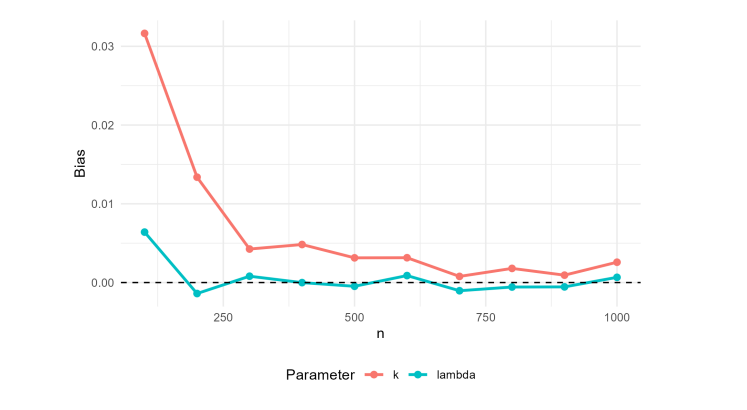
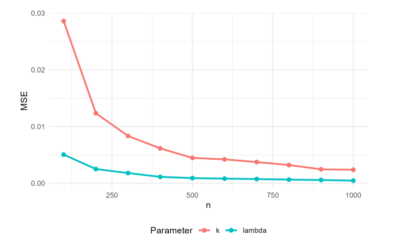
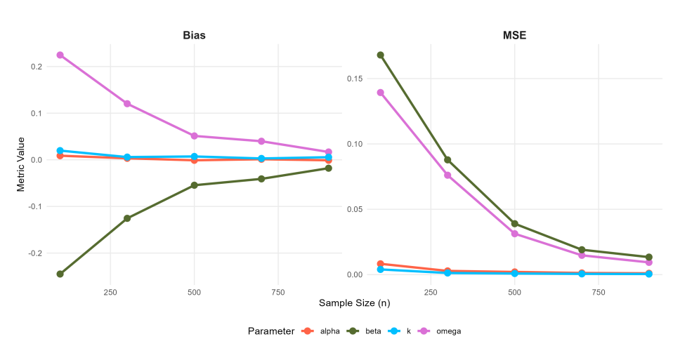
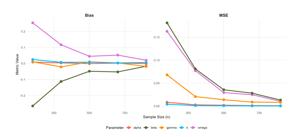
The frequentist simulation results for the SW, SW–ACD, and SW–ACD–X models are summarized in Tables 1, 2, and 3, and visualized in Figures 5, 6, 7, and 8. The results indicate that while the MLEs are asymptotically consistent, they are not uniformly robust across all sample sizes. In the small-sample regime (\(n=100\)), the dynamic SW–ACD and SW–ACD–X models exhibit sizable biases, particularly for the intercept \(\omega\) (positive bias \(\approx 0.25\)) and the persistence parameter \(\beta_1\) (negative bias \(\approx -0.26\)). These outcomes reflect an identification challenge in sparse data environments, where the estimator struggles to disentangle baseline durations from Autoregressive clustering. Conversely, in the larger sample regime (\(n \ge 700\)), both bias and MSE diminish significantly, with absolute values approaching zero by \(n=1000\). Consequently, the proposed estimators are dependable for asymptotic inference and confidence interval generation, provided the sample size is sufficiently large to mitigate these inherent small-sample biases.
| \(\lambda\) | \(k\) | |||
|---|---|---|---|---|
| \(n\) | Bias | MSE | Bias | MSE |
| 100 | 0.0064 | 0.0051 | 0.0316 | 0.0286 |
| 200 | -0.0014 | 0.0025 | 0.0134 | 0.0124 |
| 300 | 0.0008 | 0.0018 | 0.0043 | 0.0083 |
| 400 | 0.0000 | 0.0011 | 0.0048 | 0.0062 |
| 500 | -0.0005 | 0.0009 | 0.0031 | 0.0045 |
| 600 | 0.0009 | 0.0008 | 0.0032 | 0.0042 |
| 700 | -0.0010 | 0.0008 | 0.0008 | 0.0037 |
| 800 | -0.0006 | 0.0006 | 0.0018 | 0.0032 |
| 900 | -0.0006 | 0.0006 | 0.0009 | 0.0025 |
| 1000 | 0.0007 | 0.0005 | 0.0026 | 0.0024 |
| \(\omega\) | \(\alpha_1\) | \(\beta_1\) | \(k\) | |||||
|---|---|---|---|---|---|---|---|---|
| \(n\) | Bias | MSE | Bias | MSE | Bias | MSE | Bias | MSE |
| 100 | 0.2247 | 0.1393 | 0.0088 | 0.0083 | -0.2449 | 0.1680 | 0.0198 | 0.0040 |
| 300 | 0.1203 | 0.0761 | 0.0032 | 0.0028 | -0.1255 | 0.0878 | 0.0058 | 0.0012 |
| 500 | 0.0512 | 0.0313 | -0.0010 | 0.0020 | -0.0545 | 0.0390 | 0.0072 | 0.0008 |
| 700 | 0.0398 | 0.0147 | 0.0012 | 0.0013 | -0.0409 | 0.0190 | 0.0029 | 0.0006 |
| 900 | 0.0168 | 0.0094 | -0.0010 | 0.0010 | -0.0180 | 0.0134 | 0.0056 | 0.0004 |
| \(\omega\) | \(\alpha_1\) | \(\beta_1\) | \(\gamma_1\) | \(k\) | ||||||
|---|---|---|---|---|---|---|---|---|---|---|
| \(n\) | Bias | MSE | Bias | MSE | Bias | MSE | Bias | MSE | Bias | MSE |
| 100 | 0.2533 | 0.1628 | 0.0090 | 0.0085 | -0.2650 | 0.1813 | 0.0109 | 0.0682 | 0.0250 | 0.0043 |
| 300 | 0.1167 | 0.0773 | 0.0036 | 0.0029 | -0.1124 | 0.0811 | -0.0216 | 0.0208 | 0.0073 | 0.0013 |
| 500 | 0.0447 | 0.0295 | -0.0008 | 0.0021 | -0.0484 | 0.0357 | 0.0101 | 0.0140 | 0.0081 | 0.0009 |
| 700 | 0.0522 | 0.0249 | 0.0022 | 0.0013 | -0.0525 | 0.0283 | 0.0037 | 0.0090 | 0.0035 | 0.0006 |
| 900 | 0.0202 | 0.0106 | -0.0007 | 0.0010 | -0.0172 | 0.0133 | -0.0189 | 0.0083 | 0.0062 | 0.0005 |
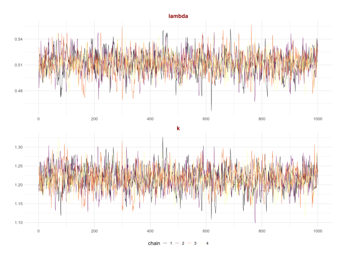
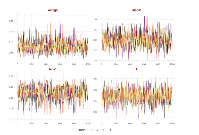
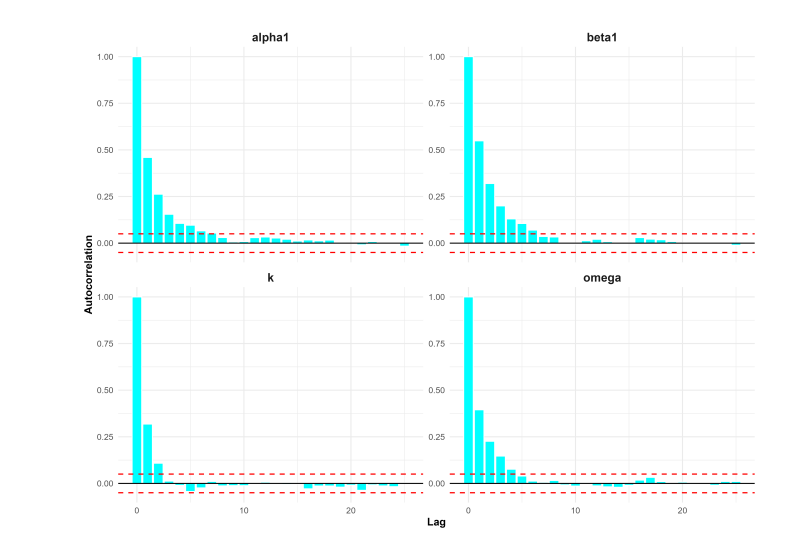
The Bayesian estimation results for the SW, SW–ACD, and SW–ACD–X models Table 4 demonstrates a highly reliable and robust framework. MCMC diagnostics confirm numerical stability and convergence across all specifications. Specifically, the trace plots Figures 9 to 11 show well-mixed chains, and the autocorrelation plots Figures 12 to 14 exhibit rapid decay, ensuring that the posterior samples are independent. This stability is further supported by \(\hat{R}\) values near 1.00 and high effective sample sizes (\(n_{\text{eff}} > 1000\)). Furthermore, parameter recovery is highly accurate; posterior means closely match the true values and fall within the 95% credible intervals. Notably, the successful identification of the calendar effect (\(\gamma_1\)) in the SW-ACD-X model proves that the framework is computationally efficient and statistically sound for application to real-world high-frequency financial data.
| Model | Parameter | Mean | SD | 2.5% | 50% | 97.5% | \(n_{\text{eff}}\) | Rhat |
|---|---|---|---|---|---|---|---|---|
| SW | \(\lambda\) | 0.5119 | 0.0130 | 0.4843 | 0.5122 | 0.5372 | 1132 | 1.0044 |
| \(k\) | 1.2167 | 0.0302 | 1.1554 | 1.2167 | 1.2751 | 1173 | 1.0043 | |
| SW–ACD | \(\omega\) | 0.0799 | 0.0264 | 0.0360 | 0.0773 | 0.1383 | 1415 | 1.0011 |
| \(\alpha_1\) | 0.0797 | 0.0129 | 0.0566 | 0.0789 | 0.1069 | 1059 | 1.0028 | |
| \(\beta_1\) | 0.8212 | 0.0307 | 0.7560 | 0.8229 | 0.8762 | 1019 | 1.0027 | |
| \(k\) | 1.2205 | 0.0302 | 1.1608 | 1.2196 | 1.2808 | 2092 | 1.0020 | |
| SW–ACD–X | \(\omega\) | 0.0966 | 0.0268 | 0.0514 | 0.0944 | 0.1561 | 1753 | 1.0001 |
| \(\alpha_1\) | 0.1141 | 0.0141 | 0.0873 | 0.1136 | 0.1449 | 1478 | 1.0012 | |
| \(\beta_1\) | 0.7479 | 0.0326 | 0.6791 | 0.7498 | 0.8076 | 1280 | 1.0010 | |
| \(\gamma_1\) | 0.0634 | 0.0192 | 0.0256 | 0.0635 | 0.0999 | 3169 | 1.0016 | |
| \(k\) | 1.1718 | 0.0290 | 1.1170 | 1.1712 | 1.2296 | 3114 | 1.0000 |
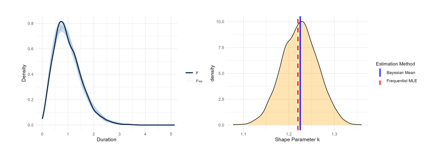
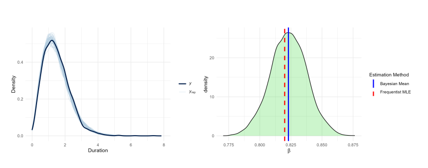
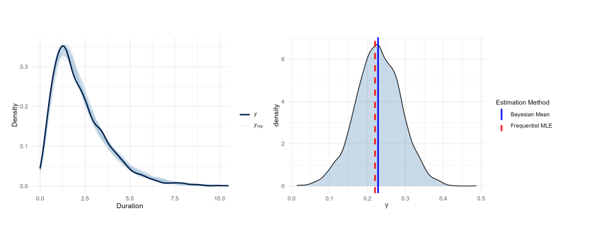
Posterior predictive checks confirm the structural adequacy of the Secant-Weibull specifications, with generated densities closely matching observed data. High estimation consistency is evidenced by the near-perfect alignment between frequentist MLEs (red dashed lines) and Bayesian posterior means (blue solid lines).
As shown in Figure 15, the model successfully recovers the shape parameter \(k\) while validating the trigonometric density. Figure 16 demonstrates similar precision for the persistence parameter \(\beta_1\), where the MLE coincides with the posterior peak. Finally, Figure 17 confirms that the SW-ACD-X model accurately identifies the exogenous calendar effect \(\gamma_1\). This convergence across all parameters (\(k, \beta_1, \gamma_1\)) highlights the numerical stability and superior generative performance of the proposed framework.
This section presents the empirical application of the SW-ACD-X model to high-frequency IBM transaction data. We conduct a comparative analysis against benchmarks like W–ACD–X, LW–ACD–X, Lomax–ACD–X, and G–ACD–X models, validating our specification through Frequentist and Bayesian frameworks. We assess model performance using the AIC and BIC for maximum likelihood, along with the WAIC and LOOIC for posterior analysis. This dual-method approach rigorously tests the SW–ACD–X model’s efficiency in capturing heavy-tailed innovations and intraday calendar effects
The empirical study utilizes 3,534 IBM transaction durations (\(x_i\)) sampled from the
ibm.txt dataset covering November 1–7, 1990. After removing
overnight gaps to isolate active trading sessions. Table 5 shows that the series displays
high variability and positive skewness, meaning that most durations are
short but occasionally very long. The density plot in Figure 18 supports this finding,
revealing a clearly right-skewed and leptokurtic distribution. These
features indicate heavy-tailed behavior, where extreme durations occur
more often than under normality.
In terms of temporal dependence, the autocorrelation function in Figure 19 shows significant persistence across several lags, reflecting strong duration clustering and long-memory effects. Additionally, Figure 20 highlights clear intraday seasonality, with trading activity following a U-shaped pattern high at the market open and close and lower during midday.
| Statistic | Mean | Median | Std. Dev | Minimum | Maximum | Skewness | Kurtosis |
|---|---|---|---|---|---|---|---|
| Duration | 32.913 | 19 | 41.788 | 1 | 466 | 2.99 | 14.00 |
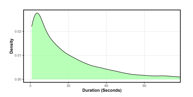
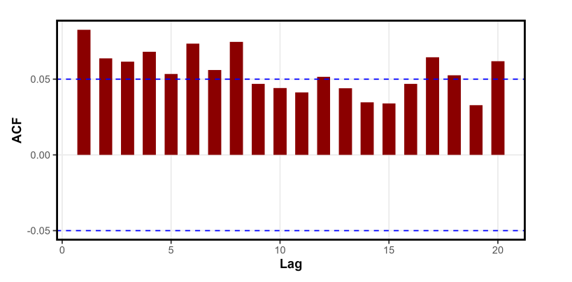
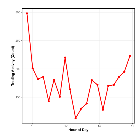
Table 6 demonstrates that the parameters are statistically significant for all five ACD–X frameworks, and the total of \(\alpha_1\) and \(\beta_1\) are constantly approaching unity to suggest great duration persistence. Additionally, a persistent calendar effect is shown by the large negative estimates for \(\gamma_1\), underscoring the significance of exogenous intraday seasonality in understanding duration dynamics.
| Model | Parameter | Estimate | Standard Error |
|---|---|---|---|
| SW–ACD–X | \(\omega\) | 0.039945 | 0.00582501 |
| \(\alpha_1\) | 0.061808 | 0.00638065 | |
| \(\beta_1\) | 0.899111 | 0.00003311 | |
| \(\gamma_1\) | \(-0.006380\) | 0.00218803 | |
| \(k\) | 0.562063 | 0.00728921 | |
| Lomax–ACD–X | \(\omega\) | 0.038920 | 0.00584951 |
| \(\alpha_1\) | 0.062239 | 0.00644485 | |
| \(\beta_1\) | 0.900361 | 0.00003315 | |
| \(\gamma_1\) | \(-0.006119\) | 0.00219196 | |
| \(k\) | 4.634004 | 0.48441160 | |
| W–ACD–X | \(\omega\) | 0.041658 | 0.00572901 |
| \(\alpha_1\) | 0.062016 | 0.00627033 | |
| \(\beta_1\) | 0.896670 | 0.00003302 | |
| \(\gamma_1\) | \(-0.007084\) | 0.00216018 | |
| \(k\) | 0.877165 | 0.01126426 | |
| LW–ACD–X | \(\omega\) | 0.040860 | 0.0062359 |
| \(\alpha_1\) | 0.062842 | 0.0088468 | |
| \(\beta_1\) | 0.878802 | 0.0209124 | |
| \(\gamma_1\) | \(-0.010831\) | 0.0034417 | |
| \(k\) | 0.880423 | 0.0112986 | |
| G–ACD–X | \(\omega\) | 0.007753 | 0.00205410 |
| \(\alpha_1\) | 0.010645 | 0.00171512 | |
| \(\beta_1\) | 0.842204 | 0.02467935 | |
| \(\gamma_1\) | \(-0.001715\) | 0.00052593 | |
| \(k\) | 0.100000 | 0.00915312 |
Table 7 summarizes the SW–ACD–X model’s performance in comparison to rival specifications. With the highest log-likelihood and the lowest information criteria values, the SW–ACD–X model exhibits superior fit and simplicity based on the Log-Likelihood, AIC, and BIC. Additionally, strong p-values from the Ljung-Box diagnostic tests show that the model effectively takes duration clustering into account and leaves the standardized residuals free of significant autocorrelation.
| Model | LogLik | AIC | BIC | LB_Stat | LB_pVal |
|---|---|---|---|---|---|
| SW–ACD–X | \(-3337.39\) | 6684.78 | 6715.63 | 5.12 | 0.883 |
| Lomax–ACD–X | \(-3347.85\) | 6705.71 | 6736.56 | 5.15 | 0.881 |
| W–ACD–X | \(-3362.83\) | 6735.65 | 6766.50 | 5.16 | 0.880 |
| LW–ACD–X | \(-3362.83\) | 6735.65 | 6766.50 | 5.16 | 0.880 |
| G–ACD–X | \(-3561.47\) | 7132.94 | 7163.79 | 9.37 | 0.497 |
This section summarizes the posterior distributions and convergence diagnostics for the proposed SW–ACD–X model and its benchmarks, confirming the stability and efficiency of the Bayesian estimation process across all specifications.
Table 8 reports the posterior estimates of the ACD–X models under different distributional assumptions. Across all specifications, the persistence parameters indicate strong duration dependence, with \(\alpha_1+\beta_1\) remaining close to unity. The posterior means are well identified with reasonably tight credible intervals for most parameters. The covariate effect \(\gamma_1\) is positive across all models, indicating a consistent influence of exogenous information on conditional durations. Convergence diagnostics are satisfactory for all models, as reflected by large effective sample sizes (neff) and \(\hat{R}\) values close to one.
| Model | Param. | Mean | SD | 2.5% | 50% | 97.5% | \(n_{\text{eff}}\) | \(\hat{R}\) |
|---|---|---|---|---|---|---|---|---|
| SW–ACD–X | \(\omega\) | 0.0220 | 0.0065 | 0.0114 | 0.0212 | 0.0371 | 1328 | 1.0035 |
| \(\alpha_1\) | 0.0289 | 0.0045 | 0.0205 | 0.0287 | 0.0386 | 1396 | 1.0023 | |
| \(\beta_1\) | 0.8783 | 0.0220 | 0.8286 | 0.8803 | 0.9149 | 1142 | 1.0043 | |
| \(\gamma_1\) | -0.0036 | 0.0015 | -0.0069 | -0.0034 | -0.0012 | 1844 | 1.0021 | |
| \(k\) | 0.5611 | 0.0074 | 0.5464 | 0.5611 | 0.5756 | 1852 | 1.0003 | |
| W–ACD–X | \(\omega\) | 0.0466 | 0.0137 | 0.0247 | 0.0445 | 0.0782 | 1575 | 1.0003 |
| \(\alpha_1\) | 0.0645 | 0.0101 | 0.0463 | 0.0638 | 0.0859 | 1681 | 1.0011 | |
| \(\beta_1\) | 0.8895 | 0.0198 | 0.8456 | 0.8918 | 0.9218 | 1390 | 1.0009 | |
| \(\gamma_1\) | -0.0079 | 0.0032 | -0.0150 | -0.0076 | -0.0027 | 1986 | 0.9993 | |
| \(k\) | 0.8766 | 0.0112 | 0.8544 | 0.8766 | 0.8981 | 2112 | 1.0017 | |
| LW–ACD–X | \(\omega\) | 0.0416 | 0.0133 | 0.0200 | 0.0400 | 0.0719 | 1166 | 1.0026 |
| \(\alpha_1\) | 0.0666 | 0.0115 | 0.0461 | 0.0658 | 0.0907 | 1357 | 1.0022 | |
| \(\beta_1\) | 0.9072 | 0.0175 | 0.8688 | 0.9088 | 0.9372 | 1022 | 1.0035 | |
| \(\gamma_1\) | -0.0043 | 0.0028 | -0.0107 | -0.0040 | 0.0007 | 1684 | 1.0027 | |
| \(k\) | 1.3016 | 0.0151 | 1.2720 | 1.3016 | 1.3319 | 1891 | 1.0015 | |
| G–ACD–X | \(\omega\) | 0.0480 | 0.0119 | 0.0273 | 0.0469 | 0.0741 | 1183 | 1.0023 |
| \(\alpha_1\) | 0.0653 | 0.0091 | 0.0491 | 0.0646 | 0.0844 | 1286 | 1.0015 | |
| \(\beta_1\) | 0.8890 | 0.0171 | 0.8523 | 0.8903 | 0.9184 | 976 | 1.0031 | |
| \(\gamma_1\) | -0.0084 | 0.0028 | -0.0145 | -0.0081 | -0.0035 | 1662 | 1.0011 | |
| \(b\) | 0.0112 | 0.0011 | 0.0100 | 0.0109 | 0.0142 | 2537 | 1.0013 | |
| Lomax–ACD–X | \(\omega\) | 0.0446 | 0.0133 | 0.0231 | 0.0431 | 0.0749 | 1523 | 1.0010 |
| \(\alpha_1\) | 0.0653 | 0.0105 | 0.0462 | 0.0649 | 0.0866 | 1623 | 1.0017 | |
| \(\beta_1\) | 0.8921 | 0.0194 | 0.8497 | 0.8939 | 0.9258 | 1369 | 1.0017 | |
| \(\gamma_1\) | -0.0070 | 0.0031 | -0.0141 | -0.0067 | -0.0019 | 1954 | 0.9996 | |
| \(k\) | 4.6553 | 0.4796 | 3.8342 | 4.6212 | 5.6779 | 2053 | 1.0007 |
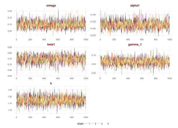
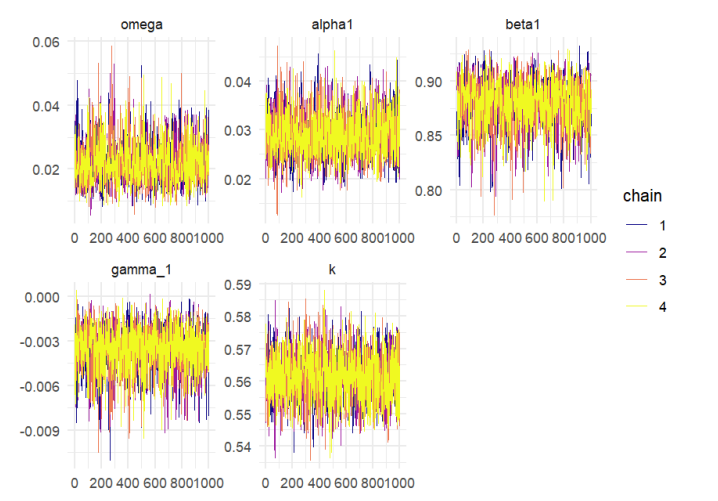
Figure 21 shows the trace plots of the parameters for the proposed SW–ACD–X model. The chains move smoothly around constant levels and mix well across all iterations, which indicates that the MCMC algorithm has successfully converged to the target posterior distribution.
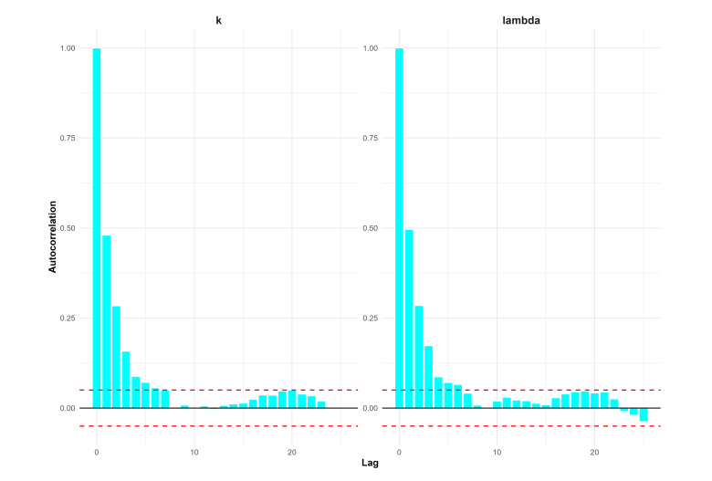
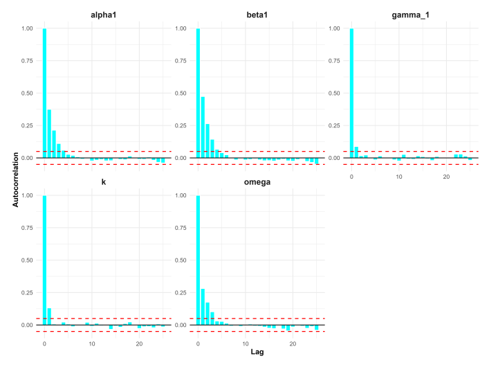
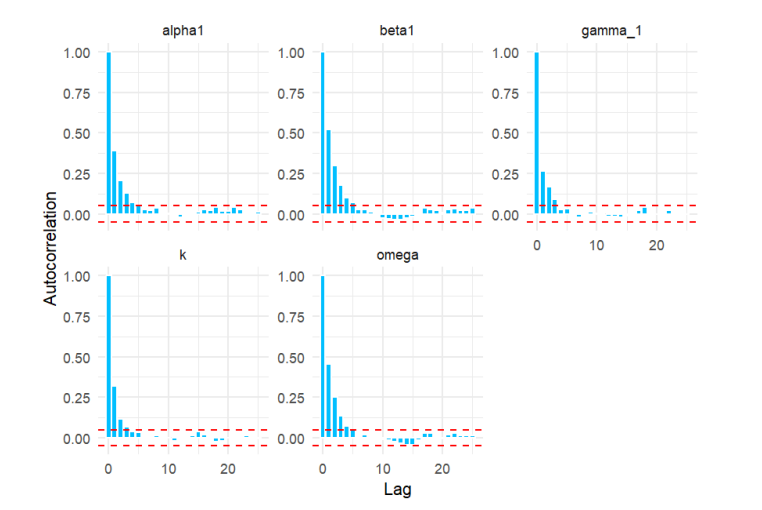
Figure 22 presents the corresponding autocorrelation function (ACF) plots. These plots show that autocorrelation decreases quickly and approaches zero after only a few lags. Together, the stable trace plots and low autocorrelation confirm the efficiency of the NUTS sampler and support the reliability of the Bayesian parameter estimates for the proposed model.
This study utilizes a Bayesian approach to model transaction duration data, estimating model parameters based on suitably defined prior distributions. We perform a comprehensive comparative analysis of five Autoregressive conditional duration specifications: W–ACD–X, LW–ACD–X , G–ACD–X, Lomax–ACD–X, and the newly introduced SW–ACD–X model.
To assess model adequacy and predictive capability, we calculate the LOOIC using posterior samples derived from Stan. As noted by [13], LOOIC serves as a robust metric for Bayesian model selection. Additionally, in line with the suggestions of [14], we also compute the WAIC to further validate the LOOIC findings.
The most efficient model in this model selection framework is the one with the lowest information criterion values. The SW–ACD–X consistently achieves the lowest LOOIC and WAIC scores when compared to the other models, according to the empirical data, which are given in Table 9. Consequently, the SW–ACD–X model exhibits the lowest LOOIC and WAIC values, indicating that it provides the best fit for capturing the duration data when calendar effects are incorporated.
| Model | WAIC | LOOIC |
|---|---|---|
| SW-ACD-X | 6693.245 | 6693.258 |
| Lomax -ACD-X | 6706.116 | 6706.127 |
| W-ACD-X | 6736.272 | 6736.286 |
| LW-ACD-X | 6729.241 | 6729.25 |
| G- ACD-X | 6867.873 | 6867.89 |
The empirical findings of this study provide a promising case for the adoption of the SW–ACD–X framework in high-frequency financial modeling. By synthesizing advances in trigonometric distribution theory with the Autoregressive Conditional Duration structure, this model seeks to bridge the gap between statistical flexibility and econometric tractability. Our analysis indicates that the framework offers several advantages over traditional duration models, serving as a robust tool for capturing the complex dynamics of irregularly spaced transaction data.
The performance of the model is rooted in the flexibility of the Secant-Weibull innovation distribution. While standard ACD models, such as the Weibull–ACD, are typically restricted by monotonic hazard functions, the SW–ACD–X inherits the ability to capture non-monotonic conditional intensities. The visual and statistical evidence suggests that the secant-transformed Weibull effectively accommodates unimodal and bathtub-shaped intensities. In a market context, the bathtub-shaped trajectory is particularly relevant; it suggests that during extended periods without transactions, the probability of a trade occurring may decrease a phenomenon frequently associated with “stale” market conditions or periods of low liquidity.
Furthermore, the endogenous treatment of calendar effects represents an integrated methodological approach. While traditional two-step filtering procedures often assume independence between intraday seasonality and stochastic duration dynamics, our joint estimation strategy suggests these components are interlinked. By estimating the calendar-effect coefficients (\(\gamma_1\)) simultaneously with the Autoregressive parameters (\(\alpha_1, \beta_1\)), the SW–ACD–X seeks to capture the interaction between deterministic diurnal patterns and stochastic clustering, providing a unified representation of the data-generating process.
From a statistical standpoint, the consistency between the Frequentist (MLE) and Bayesian (HMC–NUTS) results supports the numerical stability of the framework. In the reported IBM application, the SW–ACD–X model shows promising fit advantages as demonstrated by the AIC, BIC, WAIC, and LOOIC scores. The improvement in these information criteria over established benchmarks suggests that the added complexity of the secant transformation and exogenous variables is justified by the gain in model fit and statistical adequacy.
Our findings, supported by Monte Carlo simulations and empirical application, demonstrate the potential of the Bayesian HMC–NUTS sampler for this class of models. While the SW–ACD–X offers a robust framework for liquidity analysis, additional validation across diverse assets and market conditions is necessary to establish its broad practical superiority for trading and risk management. Future research may extend this framework to a multivariate context to explore the co-dependencies of durations across multiple assets, or incorporate volatility duration interactions to further refine our understanding of market microstructure dynamics.