
In recent years, many researchers have developed various methods for generating flexible continuous distributions due to their wide range of applications in fields such as physics, biology, medicine, finance, economics, and engineering. These distributions provide greater flexibility, allowing for more accurate modeling of different real-world phenomena. Consequently, a broad spectrum of parameter extension techniques has been proposed, leading to the development of numerous new families of probability distributions. Among the most prominent examples of these generalized families are the exponentiated-G by Gupta and Kundu [1], beta-G by Eugene et al. [2], Weibull-G by Bourguignon et al. [3], the Topp-Leone-G (TL-G) by Al-Shomrani et al. [4], the logistic-X by Tahir et al. [5], generalized TL-G by Mahdavi [6], the generalized transmuted family-G by Alizadeh et al. [7], the Marshall-Olkin half logistic-G by Makubate et al. [8], the beta odd Lindley-G by Chipepa et al. [9], the exponential Lindley odd log-logistic-G by Korkmaz et al. [10], type I half-logistic (TIHL) exponentiated-G by Bello et al. [11], the TIHL Burr X-G by Algarni et al. [12], the new TL-G by Hassan et al. [13], the xgamma-G by Cordeiro et al. [14], odd inverted Topp-Leone-G by Hassan et al. [15], odd Chen-G by Anzagra et al. [16] and others.
A recent approach aims to construct families of continuous distributions by applying trigonometric transformations and their inverses; these functions improve the performance of the model without requiring additional parameters. The main advantage of trigonometric transformations lies in their ability to strengthen the properties of the resulting distribution while maintaining a simple model structure. For example, the sine-G family by Mahmood et al. [17], the cosine-G family by Souza et al. [18], the new transformed sine-G family by Osi et al. [19], the arctan-G family by Gomez-Deniz and Calderin-Ojeda [20], the sine Topp-Leone (STL)-G family by Al-Babtain et al. [21], several recent models that have been developed using trigonometric transformations, including the sine inverted exponentiated Weibull distribution by Hassan et al. [22], the sine power unit inverse Lindley distribution by Hassan et al. [23], the arctan inverse Weibull distribution by Alrashidi [24], the sine Kumaraswamy Shanker distribution by Almetwally et al. [25], the arctan Lomax distribution by Chaudhary and Kumar [26], the sine inverted exponentiated Pareto by Hassan et al. [27], and the tangent exponentiated odd log-logistic Weibull model by Mustpha et al. [28].
In this paper, we focus on the sine Topp–Leone–G (STL-G) family, which is a new trigonometric family obtained by combining the well-known sine-G and Topp–Leone generated (TL-G) families, which inspired the name STL-G family. We show that the STL-G family possesses distinctive mathematical and practical properties, making it highly applicable for data analysis, as stated in Al-Babtain et al. [21]. The cumulative distribution function (CDF) and the probability density function (PDF) of the STL-G are determined by the following expressions: \[\label{1} F_{STL-G}(t;\phi)=\sin\Big[\frac{\pi}{2}\Big(1-\big(1-G(t;\phi)\big)^2\Big)^\lambda\Big],\hspace{4cm}t\in R, \tag{1}\] and \[\label{2} \begin{aligned} f_{STL-G}(t;\phi)=\pi\lambda& g(t;\phi)\big(1-G(t;\phi)\big)\Big[1-\big(1-G(t;\phi)\big)^2\Big]^{\lambda-1} \times\cos\Big[\frac{\pi}{2}\Big(1-\big(1-G(t;\phi)\big)^2\Big)^\lambda\Big],\hspace{1cm}t\in R, \end{aligned} \tag{2}\] where \(G(t;\phi)\) and \(g(t;\theta)\) symbolize the CDF and the PDF of any baseline distribution, \(\phi\) is the set of parameters, and \(\lambda\) is the shape parameter.
In this study, we consider the length-biased truncated Lomax (LBTL) distribution as the baseline model. This distribution was proposed by Hassan et al. [29]. The LBTL distribution is a flexible statistical model obtained by combining the concept of length-biased weighted distributions with the truncated Lomax distribution. Its importance lies in its strong ability to model positive bounded data exhibiting pronounced right skewness, particularly in situations where the probability of observation is influenced by the magnitude or duration of the underlying phenomenon. The LBTL distribution is characterized by its simplicity, as it involves only one parameter, while still maintaining considerable flexibility in the shapes of its probability density function and hazard rate function. Specifically, it is capable of modeling increasing hazard rates and unimodal density shapes, making it well suited for applications in reliability analysis, survival studies, medical research, and economic data analysis. The CDF and PDF of the LBTL distribution are expressed as follows: \[\label{3} G(t;\alpha)=C(\alpha)\Big[\big(1+t\big)^{-\alpha}\big(1+\alpha t\big)-1\Big], \hspace{2 cm} 0<t<1,\quad \alpha>0,\alpha \neq 1, \tag{3}\] and \[\label{4} g(t;\alpha)=\alpha C(\alpha)(1-\alpha)t\big(1+t\big)^{-(\alpha+1)}, \hspace{2 cm} 0<t<1,\quad \alpha>0, \alpha \neq 1, \tag{4}\] where \(C(\alpha)=\frac{1}{2^{-\alpha}(1+\alpha)-1}\), and \(\alpha\) is the shape parameter. We applied the STL-G transformation to the LBTL distribution because:
It increases the flexibility of the density function, allowing for different levels of skewness and a single-peaked (unimodal) structure.
It provides a flexible form for the hazard rate function, which in this study exhibits an increasing behavior.
The enhanced model becomes more suitable for reliability analysis, survival studies, medical research, and economic data, which often require flexible modeling of positive data.
No previous research has applied the STL-G transformation to the LBTL distribution, making this study a novel contribution.
In this research, notable progress is achieved in developing the STL-G family by integrating it with the recently proposed LBTL distribution, leading to the introduction of the sine Topp-Leone length biased truncated Lomax (STLLBTL) distribution. The primary aim of the STLLBTL distribution is to improve the performance and flexibility of the LBTL distribution across a variety of datasets. We investigate the structural properties of the STLLBTL distribution, including its quantile function (QF), linear representation of the density function, moments, incomplete moments, and entropy measures (Renyi and Tsallis). This paper examines both maximum likelihood (ML) and Bayesian approaches for parameter estimation. Within the Bayesian framework, several loss functions are considered, including the squared error (SE), linear exponential (LINEX), and minimum expected loss function (MLF), under both informative prior (INP) and non-informative prior (NINP) distributions. Markov Chain Monte Carlo (MCMC) techniques are employed to carry out the required computations, and the performance of the proposed estimation methods is assessed through Monte Carlo simulation studies. Applications to two real datasets are presented to demonstrate the superior performance of the STLLBTL distribution over competing models. The study concludes by emphasizing the overall efficiency and robustness of the proposed distribution.
The paper is structured as follows: §2 introduces the STLLBTL distribution, while §3 discusses its mathematical properties. Methods for parameter estimation are presented in §4, followed by simulation studies in §5 to assess the performance of the proposed estimators. §6 illustrates the flexibility and practical relevance of the STLLBTL model through applications to two real datasets. Finally, §7 concludes the paper with key remarks.
The PDF of the STLLBTL distribution, with shape parameters \(\alpha>0,\alpha \neq 1\) and \(\lambda>0\), is obtained by substituting Eqs. (3) and (4) into Eq. (2), yielding the following expression: \[\label{5} \begin{aligned} f_{STLLBTL}(t;\phi)=&\pi\lambda\alpha C(\alpha)(1-\alpha)t(1+t)^{-(\alpha+1)}\Big(1-G(t;\alpha)\Big)\Big[1-\Big(1-G(t;\alpha)\Big)^2\Big]^{\lambda-1}\\& \times \cos\Bigg(\frac{\pi}{2}\Big[1-\Big(1-G(t;\alpha)\Big)^2\Big]^\lambda\Bigg),\hspace{2 cm} 0<t<1, \end{aligned} \tag{5}\] and the CDF of the STLLBTL distribution is obtained by substituting Eq. (3) into Eq. (1), yielding the following expression: \[\label{6} F_{STLLBTL}(t;\phi)=\sin\Bigg(\frac{\pi}{2}\Big[1-\Big(1-G(t;\alpha)\Big)^2\Big]^\lambda\Bigg),\hspace{1 cm} 0<t<1,\quad \lambda>0, \alpha>0,\alpha \neq 1, \tag{6}\] where \(\phi=(\alpha,\lambda)^T\) denotes the set of parameters, with \(\alpha\) and \(\lambda\) are the shape parameters.
The survival function, hazard rate function (HRF) and reversed HRF of STLLBTL distribution are shown below: \[\label{7} S_{STLLBTL}(t;\phi)=1-\sin\Bigg(\frac{\pi}{2}\Big[1-\Big(1-G(t;\alpha)\Big)^2\Big]^\lambda\Bigg),\hspace{1 cm} 0<t<1,\quad \lambda>0, \alpha>0,\alpha \neq 1, \tag{7}\] \[\begin{aligned} &h_{STLLBTL}(t;\phi)=\\&\frac{\pi\lambda\alpha C(\alpha)(1-\alpha)t(1+t)^{-(\alpha+1)}\Big(1-G(t;\alpha)\Big)\Big[1-\Big(1-G(t;\alpha)\Big)^2\Big]^{\lambda-1} \cos\Bigg(\frac{\pi}{2}\Big[1-\Big(1-G(t;\alpha)\Big)^2\Big]^\lambda\Bigg)}{1-\sin\Bigg(\frac{\pi}{2}\Big[1-\Big(1-G(t;\alpha)\Big)^2\Big]^\lambda\Bigg)}, \end{aligned} \tag{8}\] and \[\begin{aligned} &r_{STLLBTL}(t;\phi)=\\&\pi\lambda\alpha C(\alpha)(1-\alpha)t(1+t)^{-(\alpha+1)}\Big(1-G(t;\alpha)\Big)\Big[1-\Big(1-G(t;\alpha)\Big)^2\Big]^{\lambda-1} \cot\Bigg(\frac{\pi}{2}\Big[1-\Big(1-G(t;\alpha)\Big)^2\Big]^\lambda\Bigg). \end{aligned} \tag{9}\]
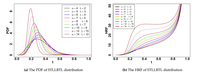
The PDF may exhibit a single peak and right skewness, while the HRF can display an increasing trend, as illustrated in Figure 1.
This section presents the principal statistical properties of the STLLBTL distribution, including the linear representation of the PDF, QF, moments, incomplete moments, and entropy measures.
This subsection provides a detailed expansion of the PDF of the newly developed distribution, facilitating a comprehensive analysis of the structural properties of the STLLBTL distribution. We will use the Maclaurin series expansion of the cosine function: \[\label{8} \cos y=\sum\limits_{i=0}^{\infty}\frac{(-1)^i y^{2i}}{(2i)!}. \tag{10}\]
Then, the PDF (5) is expressed as follows: \[\label{aa} \begin{aligned} f_{STLLBTL}(t;\phi)=\sum\limits_{i=0}^{\infty}\frac{(-1)^i \pi^{2i+1}\lambda\alpha C(\alpha)(1-\alpha)}{2^{2i}(2i)!}t(1+t)^{-(\alpha+1)}\Big(1-G(t;\alpha)\Big) \Big[1-\Big(1-G(t;\alpha)\Big)^2\Big]^{2i\lambda+\lambda-1}. \end{aligned} \tag{11}\]
Using the following expansion \[\label{9} (1 – z)^b = \sum\limits_{i = 0}^\infty {\left( { – 1} \right)^i \left( {\begin{array}{*{20}c} b \\ i \\ \end{array} } \right)z^i } ,\,\,\left| z \right| < 1, \tag{12}\]
in Eq. (11) yields: \[f_{STLLBTL}(t;\phi)=\sum\limits_{i,j=0}^{\infty}\frac{(-1)^{i+j} \pi^{2i+1}\lambda\alpha C(\alpha)(1-\alpha)\binom{2i\lambda+\lambda-1}{j}}{2^{2i}(2i)!}t(1+t)^{-(\alpha+1)}\Big(1-G(t;\alpha)\Big)^{2j+1}.\]
Applying the binomial Expansion (12) once more leads to \[f_{STLLBTL}(t;\phi)=\sum\limits_{i,j,k=0}^{\infty} C_{i,j,k}^*(\alpha) \lambda t(1+t)^{-(\alpha+1)}\Big[\big(1+t\big)^{-\alpha}\big(1+\alpha t\big)-1\Big]^k,\] where \[C_{i,j,k}^*(\alpha)=\frac{(-1)^{i+j+k}\pi^{2i+1}\alpha \Big(C(\alpha)\Big)^{1+k}(1-\alpha)\binom{2i\lambda+\lambda-1}{j}\binom{2j+1}{k}}{2^{2i}(2i)!}.\]
By expanding once again, we obtain \[f_{STLLBTL}(t;\phi)=\sum\limits_{i,j,k=0}^{\infty}\sum\limits_{m=0}^{k} D_{i,j,k,m}t(1+t)^{-\alpha(1+m)-1}(1+\alpha t)^m, \] where \[D_{i,j,k,m}=C_{i,j,k}^*(\alpha)(-1)^{k-m} \lambda\binom{k}{m}.\]
By expanding the last two terms \[\label{10} f_{STLLBTL}(t;\phi)=\sum\limits_{i,j,k,d=0}^{\infty}\sum\limits_{m=0}^{k}\sum\limits_{l=0}^{m}B_{i,j,k,m,l,d}t^{l+d+1}, \tag{13}\] where \[B_{i,j,k,m,l,d}=D_{i,j,k,m}(-1)^d\binom{m}{l}\binom{\alpha(1+m)+d}{d}\alpha^l.\]
The QF, also referred to as the inverse CDF, assigns to each probability level a corresponding value of the random variable. It plays a vital role in numerous statistical applications. By defining \(Q(u)=F^{-1}(u)\), where \(0<u<1\) denotes a uniformly distributed random variable, Eq. (6) can be rewritten as: \[u=\sin\Bigg(\frac{\pi}{2}\Big[1-\Big(1-\frac{\big(1+Q(u)\big)^{-\alpha}\big(1+\alpha Q(u)\big)-1}{2^{-\alpha}(1+\alpha)-1}\Big)^2\Big]^\lambda\Bigg).\]
After simplification, the QF of the STLLBTL model is \[\label{d11} \big(1+Q(u)\big)^{-\alpha}\big(1+\alpha Q(u)\big)=1+\Bigg(1-\Big[1-\Big(\frac{2}{\pi}\sin^{-1}u\Big)^{\frac{1}{\lambda}}\Big]^{\frac{1}{2}}\Bigg)\Bigg(2^{-\alpha}(1+\alpha)-1\Bigg), \hspace{8mm} u \in (0,1). \tag{14}\]
Random samples can be generated by drawing u \(\sim\) U (0,1) and numerically solving Eq. (14) using a root-finding method to obtain \(Q(u)\).
Moments are fundamental tools in probability and statistics that summarize key characteristics of a random variable. They describe the shape, central tendency, and variability of a distribution, helping to understand features such as symmetry, skewness, and kurtosis, the \(r^{th}\) moment of the STLLBTL model is given by using the PDF (13) of STLLBTL distribution as below:
\[\begin{aligned} \label{12} \mu_r'&= \int_{0}^{1} t^r f(t;\phi) dt=\sum\limits_{i,j,k,d=0}^{\infty}\sum\limits_{m=0}^{k}\sum\limits_{l=0}^{m}B_{i,j,k,m,l,d}\int_{0}^{1}t^{r+l+d+1} dt\notag\\& =\sum\limits_{i,j,k,d=0}^{\infty}\sum\limits_{m=0}^{k}\sum\limits_{l=0}^{m}\frac{B_{i,j,k,m,l,d}}{r+l+d+2}. \end{aligned} \tag{15}\]
The mean is obtained at \(r=1\): \[\mu_1'=\sum\limits_{i,j,k,d=0}^{\infty}\sum\limits_{m=0}^{k}\sum\limits_{l=0}^{m}\frac{B_{i,j,k,m,l,d}}{l+d+3}. \tag{16}\]
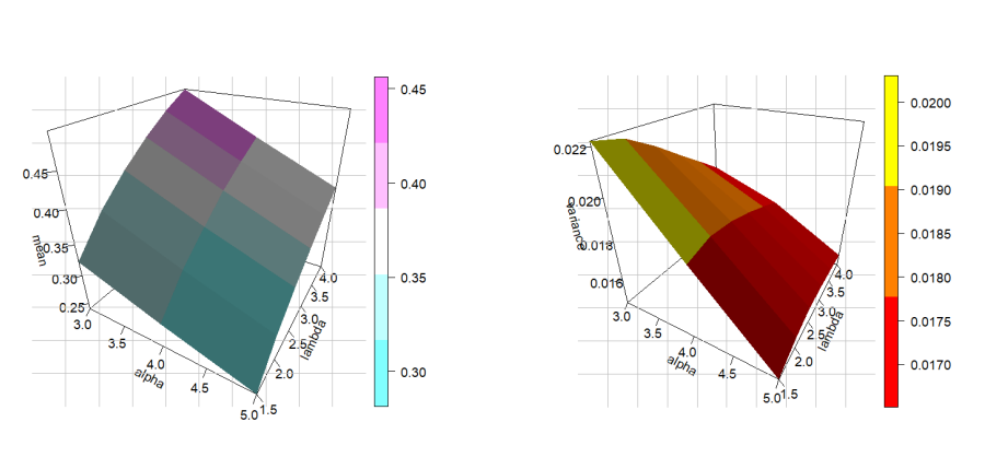
Table 1 presents the first four moments, variance (\(\sigma^2\)), skewness (S), and kurtosis (K) of the STLLBTL distribution for selected sets of parameter values.
| \(\alpha\) | \(\lambda\) | \(\mu'_1\) | \(\mu'_2\) | \(\mu'_3\) | \(\mu'_4\) | \(\sigma^2\) | S | K |
|---|---|---|---|---|---|---|---|---|
| 0.6 | 0.2 | 0.0814540 | 0.0202963 | 0.0075059 | 0.0034402 | 0.0136616 | 2.2715060 | 8.9507870 |
| 0.5 | 0.2151871 | 0.0741271 | 0.0323232 | 0.0163311 | 0.0278216 | 0.9477877 | 3.4510960 | |
| 1 | 0.3557464 | 0.1577525 | 0.0802699 | 0.0449644 | 0.0311970 | 0.3545375 | 2.5473770 | |
| 1.5 | 0.2 | 0.0695039 | 0.0154747 | 0.0052702 | 0.0022693 | 0.0106439 | 2.4724470 | 10.4386800 |
| 0.5 | 0.1868652 | 0.0579644 | 0.0233256 | 0.0110657 | 0.0230457 | 1.1093770 | 3.9860560 | |
| 1 | 0.31482590 | 0.1269290 | 0.0598556 | 0.0315171 | 0.0278137 | 0.5135428 | 2.7828520 |
Based on the results in Table 1, the following properties can be observed:
When the value of \(\alpha\) is fixed and the value of \(\lambda\) increases, we observe the following:
The values of the first four moments and the \(\sigma^2\) increase proportionally with the increase of \(\lambda\). This means that the distribution widens and its center shifts to the right.
We observe a significant decrease in the values of S and K. This indicates that the distribution becomes closer to the shape of a normal distribution (less peaked and with shorter tails) as the value of \(\lambda\) increases.
When \(\alpha\) changes while \(\lambda\) is kept fixed, we observe the following:
We observe that the values of the first four moments and the \(\sigma^2\) slightly decrease as \(\alpha\) increases.
The values of S and K are higher at \(\alpha=1.5\) compared to \(\alpha=0.6\) (for the same value of \(\lambda\)). This means that increasing \(\alpha\) makes the distribution more right-skewed and more peaked (leptokurtic).
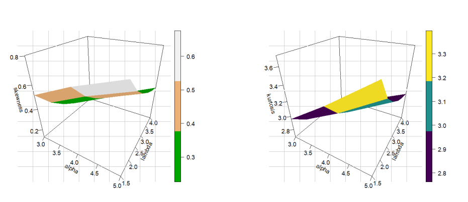
All S values in the table are positive, confirming that the STLLBTL distribution is right-skewed in all tested cases.
Most K values are much higher than 3, so the distribution is considered leptokurtic
The 3D plots of \(\mu_1'\), \(\sigma^2\), S and K measures are shown in Figures 2 and 3 to provide more clarification and explanation.
The \(r^{th}\) incomplete moment of STLLBTL distribution is obtained by using the PDF (13) as follows
\[\begin{aligned} T_r(t_{1}) &= \int_{0}^{t_{1}} t^r f(t;\phi) dt= \sum\limits_{i,j,k,d=0}^{\infty}\sum\limits_{m=0}^{k}\sum\limits_{l=0}^{m}B_{i,j,k,m,l,d}\int_{0}^{t_{1}}t^{r+l+d+1} dt =\sum\limits_{i,j,k,d=0}^{\infty}\sum\limits_{m=0}^{k}\sum\limits_{l=0}^{m} \frac{B_{i,j,k,m,l,d}}{l+d+r+2} t_{1}^{r+l+d+2}. \end{aligned} \tag{17}\]
Entropy is a key measure in information theory that quantifies uncertainty or randomness in a probability distribution and the information content of a system, refer to [30]–[32]. Shannon entropy is the classical form and forms the basis for generalized measures such as Rényi entropy [33], which introduces an order parameter for greater flexibility, and Tsallis entropy, developed for non-extensive systems. These measures are widely used to assess variability and information in probabilistic models.The Rényi entropy of the STLLBTL distribution is obtained by substituting Eq. (5) into the Rényi entropy formula
\[\label{19} \Xi(\rho)=\big(1-\rho\big)^{-1}log\Big[\int_{0}^{1}\Big(f(t;\phi)\Big)^\rho dt\Big],\hspace{2 cm} \rho>0 \quad and\quad \rho \neq 1, \tag{18}\] where \(\rho\) is the entropy order. We must obtain \(\Big(f(t;\phi)\Big)^\rho\), as follows: \[\label{20} \begin{aligned} \Big(f(t;\phi)\Big)^\rho=& (\pi\lambda)^\rho\alpha^\rho \big(C(\alpha)\big)^\rho(1-\alpha)^\rho t^\rho(1+t)^{-\rho(\alpha+1)}\Big(1-G(t;\alpha)\Big)^\rho \Big[1-\Big(1-G(t;\alpha)\Big)^2\Big]^{\rho\lambda-\rho}\\& \times \cos^\rho\Bigg(\frac{\pi}{2}\Big[1-\Big(1-G(t;\alpha)\Big)^2\Big]^\lambda\Bigg). \end{aligned} \tag{19}\]
Using the binomial theory, then \(\cos^\rho\Bigg(\frac{\pi}{2}\Big[1-\Big(1-G(t;\alpha)\Big)^2\Big]^\lambda\Bigg)\) is expanded as follows: \[\cos^\rho\Bigg(\frac{\pi}{2}\Big[1-\Big(1-G(t;\alpha)\Big)^2\Big]^\lambda\Bigg) =1+\sum\limits_{i=1}^{\infty}\binom{\rho}{i}\Big[1-\Big(1-G(t;\alpha)\Big)^2\Big]^{2\lambda i}\Bigg[\sum\limits_{k=0}^{\infty} w_{k}\Big[1-\Big(1-G(t;\alpha)\Big)^2\Big]^{2\lambda k}\Bigg]^i,\] where \(w_{k}=\frac{(-1)^{k+1} \pi^{2(k+1)}}{\big(2(k+1)\big)!2^{2(k+1)}}\). Using the power series expansion formula:
\[\Bigg( \sum\limits_{k=0}^{\infty} a_k
x^k \Bigg)^j = \sum\limits_{k=0}^{\infty} C_k x^k,\] where \(k\) is a positive integer and \(C_0 = a_0^j, \quad C_m = \left(\frac{1}{m
a_0}\right) \sum\limits_{k=1}^m (kj – m + k) a_k C_{m-k}, \quad m \geq
1.\)
We obtain the expanded form: \[\cos^\rho\Bigg(\frac{\pi}{2}\Big[1-\Big(1-G(t;\alpha)\Big)^2\Big]^\lambda\Bigg)
=1+\sum\limits_{i=1}^{\infty}\binom{\rho}{i}\sum\limits_{k=0}^{\infty}w^*_{k}\Big[1-\Big(1-G(t;\alpha)\Big)^2\Big]^{2\lambda
(k+i)},\] where \[\omega_0^* =
\omega_0^i \quad \text{and} \quad \omega_m^* = \left(\frac{1}{m
\omega_0}\right) \sum\limits_{k=1}^m (mi – m + k) \omega_k
\omega_{m-k}^*, \quad m \ge 1.\]
Then \[\label{22} \cos^\rho\Bigg(\frac{\pi}{2}\Big[1-\Big(1-G(t;\alpha)\Big)^2\Big]^\lambda\Bigg) =1+\sum\limits_{i=1}^{\infty}\sum\limits_{k=0}^{\infty}w^*_{k,i}\Big[1-\Big(1-G(t;\alpha)\Big)^2\Big]^{2\lambda (k+i)}, \tag{20}\] where \(w^*_{k,i}=\binom{\rho}{i}w^*_{k}\), substituting Eq. (20) in Eq. (19), gives \[\begin{aligned} \Big(f(t;\phi)\Big)^\rho= &At^\rho(1+t)^{-\rho(\alpha+1)}\Big(1-G(t;\alpha)\Big)^\rho \Big[1-\Big(1-G(t;\alpha)\Big)^2\Big]^{\rho\lambda-\rho}\\& \times\Bigg[1+\sum\limits_{i=1}^{\infty}\sum\limits_{k=0}^{\infty}w^*_{k,i}\Big[1-\Big(1-G(t;\alpha)\Big)^2\Big]^{2\lambda (k+i)}\Bigg], \end{aligned}\] where \(A=(\pi\lambda)^\rho\alpha^\rho \big(C(\alpha)\big)^\rho(1-\alpha)^\rho,\) then \[\label{23} \begin{aligned} \Big(f(t;\phi)\Big)^\rho=I_{1}+I_{2}, \end{aligned} \tag{21}\] where \[I_{1}=A t^\rho(1+t)^{-\rho(\alpha+1)}\Big(1-G(t;\alpha)\Big)^\rho \Big[1-\Big(1-G(t;\alpha)\Big)^2\Big]^{\rho\lambda-\rho},\] and \[\begin{aligned} I_{2}=&\sum\limits_{i=1}^{\infty}\sum\limits_{k=0}^{\infty}w^*_{k,i}A t^\rho(1+t)^{-\rho(\alpha+1)}\Big(1-G(t;\alpha)\Big)^\rho \Big[1-\Big(1-G(t;\alpha)\Big)^2\Big]^{\lambda(\rho+2k+2i)-\rho}. \end{aligned}\]
After simplification, \[\label{24} I_{1}=\sum\limits_{j,m,b=0}^{\infty}\sum\limits_{a=0}^{m}\sum\limits_{d=0}^{a}M_{j,m,b,a,d} t^{\rho+b+d}, \tag{22}\] where \[M_{j,m,b,a,d}=(-1)^{j+2m-a+b}\binom{\rho \lambda-\rho}{j}\binom{\rho+2j}{m}\binom{m}{a}\binom{\alpha(\rho+a)+\rho+b-1}{b}\binom{a}{d} A \alpha^d \big(C(\alpha)\big)^m,\]
and \[\label{25} I_{2}=\sum\limits_{i=1}^{\infty}\sum\limits_{k,e,f,n=0}^{\infty}\sum\limits_{l=0}^{f}\sum\limits_{h=0}^{l}N_{i,k,e,f,n,l,h} t^{\rho+n+h}, \tag{23}\] where \[N_{i,k,e,f,n,l,h}= (-1)^{e+2f-l+n}\binom{\lambda(\rho+2k+2i)-\rho}{e}\binom{\rho+2e}{f}\binom{f}{l}\binom{\alpha(\rho+l)+\rho+n-1}{n}\binom{l}{h} w^*_{k,i} A \alpha^h \big(C(\alpha)\big)^f.\]
Substituting Eqs. (22) and (23) in Eq. (21) \[\label{26} \begin{aligned} \Big(f(t;\phi)\Big)^\rho=\sum\limits_{j,m,b=0}^{\infty}\sum\limits_{a=0}^{m}\sum\limits_{d=0}^{a}M_{j,m,b,a,d} t^{\rho+b+d}+\sum\limits_{i=1}^{\infty}\sum\limits_{k,e,f,n=0}^{\infty}\sum\limits_{l=0}^{f}\sum\limits_{h=0}^{l}N_{i,k,e,f,n,l,h} t^{\rho+n+h}. \end{aligned} \tag{24}\]
Substituting Eq. (24) in Eq. (18) \[\Xi(\rho)=\big(1-\rho\big)^{-1}log\Bigg[\sum\limits_{j,m,b=0}^{\infty}\sum\limits_{a=0}^{m}\sum\limits_{d=0}^{a}M_{j,m,b,a,d}\int_{0}^{1} t^{\rho+b+d}dt +\sum\limits_{i=1}^{\infty}\sum\limits_{k,e,f,n=0}^{\infty}\sum\limits_{l=0}^{f}\sum\limits_{h=0}^{l}N_{i,k,e,f,n,l,h} \int_{0}^{1}t^{\rho+n+h}dt\Bigg].\]
Then the Rényi entropy of STLLBTL distribution can be written as \[\Xi(\rho)=\big(1-\rho\big)^{-1}log\Bigg[\sum\limits_{j,m,b=0}^{\infty}\sum\limits_{a=0}^{m}\sum\limits_{d=0}^{a}\frac{M_{j,m,b,a,d}}{\rho+b+d+1} +\sum\limits_{i=1}^{\infty}\sum\limits_{k,e,f,n=0}^{\infty}\sum\limits_{l=0}^{f}\sum\limits_{h=0}^{l}\frac{N_{i,k,e,f,n,l,h}}{\rho+n+h+1} \Bigg].\]
Additionally, the Tsallis entropy, presented by Tsallis [34], for the STLLBTL distribution is determined by employing the following equation \[\Xi_{1}(\rho)=\Big(1-\rho\Big)^{-1}\Big[1-\int_{0}^{1}\Big(f(t;\phi)\Big)^\rho dt\Big],\hspace{2 cm} \rho>0 \quad and \quad \rho \neq 1.\]
Using the similar procedure discussed above, then \[\Xi_{1}(\rho)=\big(1-\rho\big)^{-1}\Bigg[1-\Bigg(\sum\limits_{j,m,b=0}^{\infty}\sum\limits_{a=0}^{m}\sum\limits_{d=0}^{a}\frac{M_{j,m,b,a,d}}{\rho+b+d+1} +\sum\limits_{i=1}^{\infty}\sum\limits_{k,e,f,n=0}^{\infty}\sum\limits_{l=0}^{f}\sum\limits_{h=0}^{l}\frac{N_{i,k,e,f,n,l,h}}{\rho+n+h+1}\Bigg) \Bigg]. \tag{25}\]
Table 2 presents the entropy values, which provide a quantitative measure of the uncertainty and information content associated with the STLLBTL distribution under different parameter values. Lower entropy values indicate that the distribution is more peaked, implying less randomness and greater predictability of outcomes within the interval (0,1). In contrast, higher entropy values suggest that the distribution is more spread out, leading to a greater degree of uncertainty. For instance, when \(\alpha\) increases while \(\lambda\) is fixed, the Rényi and Tsallis entropy measures decrease, indicating reduced dispersion and increased predictability and when \(\alpha\) is fixed while \(\lambda\) increases, the entropy increases, indicating greater variability in the data. It is important to note that the negative values of Rényi and Tsallis entropies are theoretically valid in this case, since the distribution is defined on a bounded support (0,1), where the PDF may exceed one.
| \(\alpha\) | \(\lambda\) | \(\rho = 0.3\) | \(\rho =0.5\) | \(\rho =0.8\) | |||
|---|---|---|---|---|---|---|---|
| \(\Xi(\rho)\) | \(\Xi_1(\rho)\) | \(\Xi(\rho)\) | \(\Xi_1(\rho)\) | \(\Xi(\rho)\) | \(\Xi_1(\rho)\) | ||
| 0.6 | 0.2 | -0.6689968 | -0.5341899 | -1.0264742 | -0.8028903 | -1.5389199 | -1.3246295 |
| 0.5 | -0.2987588 | -0.2695874 | -0.4102927 | -0.3709438 | -0.5231584 | -0.4967190 | |
| 1 | -0.1869393 | -0.1752246 | -0.2538851 | -0.2384314 | -0.3210725 | -0.3109809 | |
| 1.5 | 0.2 | -0.7578673 | -0.5881335 | -1.1510197 | -0.8751639 | -1.6979621 | -1.4396976 |
| 0.5 | -0.3665767 | -0.3233218 | -0.5027608 | -0.4445471 | -0.6389774 | -0.5998332 | |
| 1 | -0.2292309 | -0.2117850 | -0.3095310 | -0.2867679 | -0.3884976 | -0.3737880 | |
In this section, the parameters of the STLLBTL distribution are estimated using both ML and Bayesian methods. In the Bayesian approach, several loss functions are employed, including SE, LINEX, and MLF loss functions.
Assume that a simple random sample \(\underline{\mathbf{t}} = (t_1, t_2, …, t_n)\) of size \(n\) is drawn from a population that follows the STLLBTL distribution given in Eq. (5), where the parameter vector \(\phi = (\alpha, \lambda)^T\) is unknown. The corresponding likelihood function \(L(\phi | \underline{\mathbf{t}})\) can then be expressed as follows: \[\label{28} \begin{aligned} L(\phi|\underline{\mathbf{t}})=&\pi^n\lambda^n \alpha^n \big(C(\alpha)\big)^n (1-\alpha)^n\prod_{i=1}^{n}\Bigg[t_{i}(1+t_{i})^{-(\alpha+1)}\Big(1-G(t_{i};\alpha)\Big)\Big[1-\Big(1-G(t_{i};\alpha)\Big)^2\Big]^{\lambda-1}\\& \times \cos\Bigg(\frac{\pi}{2}\Big[1-\Big(1-G(t_{i};\alpha)\Big)^2\Big]^\lambda\Bigg)\Bigg], \hspace{0.5cm}\lambda>0,\quad \alpha>0,\alpha \neq 1. \end{aligned} \tag{26}\]
The log likelihood function for \(\phi\), say \(logL(\phi|\underline{\mathbf{t}})\), will be \[\begin{aligned} \log L(\phi|\underline{\mathbf{t}})=&n\log\pi+n\log\lambda+n\log \alpha+n\log C(\alpha)+n\log(1-\alpha)+\sum\limits_{i=1}^{n}\log t_{i}-(\alpha+1)\sum\limits_{i=1}^{n}\log(1+t_{i})\\&+\sum\limits_{i=1}^{n}\log(1- G(t_{i};\alpha))+(\lambda-1)\sum\limits_{i=1}^{n}\log K(t_{i};\alpha) +\sum\limits_{i=1}^{n}\log\Bigg[ \cos\Bigg(\frac{\pi}{2}K^\lambda(t_{i};\alpha)\Bigg)\Bigg], \end{aligned}\]
where \(K(t_{i};\alpha)=1-\Big(1-G(t_{i};\alpha)\Big)^2.\) Differentiating \(logL(\phi|\underline{\mathbf{t}})\) with respect to \(\lambda\) and \(\alpha\) \[\label{29} \frac{\partial logL(\phi|\underline{\mathbf{t}})}{\partial \lambda}=\frac{n}{\lambda}+\sum\limits_{i=1}^{n}\log K(t_{i};\alpha)+\sum\limits_{i=1}^{n}\Bigg[-\frac{\pi}{2}K^\lambda(t_{i};\alpha) \log K(t_{i};\alpha)\tan\Big(\frac{\pi}{2}K^\lambda(t_{i};\alpha)\Big)\Bigg], \tag{27}\]
\[\label{30} \begin{aligned} \frac{\partial logL(\phi|\underline{\mathbf{t}})}{\partial \alpha}=&\frac{n}{\alpha}+n\frac{C'(\alpha)}{C(\alpha)}-\frac{n}{1-\alpha}-\sum\limits_{i=1}^{n}\log (1+t_{i})-\sum\limits_{i=1}^{n}\frac{G'(t_{i};\alpha)}{1-G(t_{i};\alpha)}+2(\lambda-1)\sum\limits_{i=1}^{n}\frac{\Big(1-G(t_{i};\alpha)\Big)G'(t_{i};\alpha)}{K(t_{i};\alpha)}\\& -\pi \lambda\sum\limits_{i=1}^{n}\Big(1-G(t_{i};\alpha)\Big)G'(t_{i};\alpha)K^{\lambda-1}(t_{i};\alpha)\tan\Big(\frac{\pi}{2}K^\lambda(t_{i};\alpha)\Big), \end{aligned} \tag{28}\] where \[C'(\alpha)=\frac{2^{-\alpha} (1+\alpha)\log(2)-2^{-\alpha}}{\Bigg[2^{-\alpha}(1+\alpha)-1\Bigg]^2},\] and \[\begin{aligned} G'(t_{i};\alpha)=C'(\alpha)\Big[\big(1+t_{i}\big)^{-\alpha}\big(1+\alpha t_{i}\big)-1\Big]+C(\alpha)\Big[\big(1+t_{i}\big)^{-\alpha}\Big(t_{i}-(1+\alpha t_{i}) \log (1+t_{i})\Big)\Big]. \end{aligned}\]
The ML estimators for parameters \(\lambda\) and \(\alpha\) are obtained by numerically solving Eqs. (27) and (28) after equating them to zero, using the bbmle package in the R programming environment, employing the L-BFGS-B algorithm with constraints \(\alpha>0,\alpha \neq 1\) and \(\lambda>0\).
This subsection discusses Bayesian estimation of the STLLBTL distribution with parameters \(\alpha\) and \(\lambda\). Both symmetric (SE) and asymmetric (LINEX, MLF) loss functions are considered under INP and NINP scenarios. Following El-Din et al. [35], Behairy and Al-Sayed [36], and Mahmoud et al. [37], the parameters are assumed independent, with separate gamma distributions used as priors for flexibility or convenience, the joint prior density function, denoted as \(\pi(\alpha, \lambda)\), is defined as the product of the marginal gamma densities for each parameter: \[\label{31} \pi(\phi)\propto \alpha^{a_{1}-1} \lambda^{a_{2}-1} e^{-\alpha b_{1}-\lambda b_{2}}, \hspace{4 cm} \lambda, a_{i}, b_{i}>0,\quad \alpha>0,\alpha \neq 1, \tag{29}\] where \(a_{i}, b_{i}, i=1,2\) are the hyperparameters. Incorporating the likelihood function (26) and the INP distribution (29) yields the joint posterior density function: \[\begin{aligned} \pi^*(\phi|\underline{\mathbf{t}})=& J \alpha^{n+a_{1}-1} \lambda^{n+a_{2}-1} e^{-\big(\alpha b_{1}+\lambda b_{2}\big)} \big(C(\alpha)\big)^n (1-\alpha)^n \prod_{i=1}^{n} t_{i}(1+t_{i})^{-(\alpha+1)}\Big(1-G(t_{i};\alpha)\Big)\\& \times K^{\lambda-1}(t_{i},\alpha)\cos\Bigg(\frac{\pi}{2}K^\lambda(t_{i};\alpha)\Bigg), \end{aligned}\] where \[\begin{aligned} J^{-1}=&\int_{0}^{\infty} \int_{0}^{\infty} \alpha^{n+a_{1}-1} \lambda^{n+a_{2}-1} e^{-\big(\alpha b_{1}+\lambda b_{2}\big)} \big(C(\alpha)\big)^n (1-\alpha)^n \prod_{i=1}^{n}t_{i}(1+t_{i})^{-(\alpha+1)}\Big(1-G(t_{i};\alpha)\Big)\\& \times K^{\lambda-1}(t_{i};\alpha) \cos\Bigg(\frac{\pi}{2}(K(t_{i};\alpha))\Bigg) d\alpha d\lambda. \end{aligned}\]
Then, \[\label{32} \begin{aligned} \pi^*(\phi|\underline{\mathbf{t}})&\propto \alpha^{n+a_{1}-1} \lambda^{n+a_{2}-1} e^{-\big(\alpha b_{1}+\lambda b_{2}\big)} \big(C(\alpha)\big)^n (1-\alpha)^n \prod_{i=1}^{n} t_{i}(1+t_{i})^{-(\alpha+1)}\Big(1-G(t_{i};\alpha)\Big)\\& \times K^{\lambda-1}(t_{i};\alpha) \cos\Bigg(\frac{\pi}{2}(K(t_{i};\alpha))\Bigg). \end{aligned} \tag{30}\]
The conditional posterior density function of \(\alpha\) given \(\lambda\) is \[\label{33} \begin{aligned} \pi^*(\alpha|\lambda, \underline{\mathbf{t}})\propto \alpha^{n+a_{1}-1} e^{-\alpha b_{1}}\big(C(\alpha)\big)^n (1-\alpha)^n \prod_{i=1}^{n}t_{i}(1+t_{i})^{-(\alpha+1)}\Big(1-G(t_{i};\alpha)\Big) K^{\lambda-1}(t_{i};\alpha) \cos\Bigg(\frac{\pi}{2}(K(t_{i};\alpha))\Bigg) . \end{aligned} \tag{31}\]
Also, the conditional posterior density function of \(\lambda\) given \(\alpha\) is \[\label{34} \begin{aligned} \pi^*(\lambda|\alpha,\underline{\mathbf{t}})\propto \lambda^{n+a_{2}-1} e^{-\lambda b_{2}} \prod_{i=1}^{n}t_{i}(1+t_{i})^{-(\alpha+1)}\Big(1-G(t_{i};\alpha)\Big) K^{\lambda-1}(t_{i};\alpha) \cos\Bigg(\frac{\pi}{2}(K(t_{i};\alpha))\Bigg). \end{aligned} \tag{32}\]
Traditional sampling methods cannot directly draw samples from Eqs. (31) and (32) since they cannot be represented using standard distributions. Therefore, the Metropolis–Hastings (M-H) algorithm, which is based on the MCMC method, is employed to generate estimators for the following loss functions. Under the SE loss, the Bayesian estimate of \(\phi\) is computed as follows: \[\label{35} \hat {\phi}= \int_{0}^{\infty}\int_{0}^{\infty} \phi\pi^*(\phi|\underline{\mathbf{t}}) d\alpha d\lambda. \tag{33}\]
According to the LINEX, The Bayesian estimator of \(\phi\) is obtained as follows
\[\hat {\phi}= \frac{-1}{\tau}ln\Big[\int_{0}^{\infty} \int_{0}^{\infty} e^{- \tau\phi} \pi^*(\phi|\underline{\mathbf{t}}) d\alpha d\lambda\Big], \tag{34}\] where \(\tau\) represents the direction and degree of asymmetry. According to the MLF, the Bayesian estimator of \(\phi\) is obtained as follows:
\[\label{37} \hat {\phi}=\frac{\int_{0}^{\infty} \int_{0}^{\infty}\phi^{-1} \pi^*(\phi|\underline{\mathbf{t}}) d\alpha d\lambda}{\int_{0}^{\infty} \int_{0}^{\infty}\phi^{-2} \pi^*(\phi|\underline{\mathbf{t}}) d\alpha d\lambda}. \tag{35}\]
For INP, we assign independent gamma distributions as priors for the parameters \(\alpha\) and \(\lambda\). Specifically, we define \(\alpha\) \(\sim\) gamma \((a_{1},b_{1})\) and \(\lambda\) \(\sim\) gamma \((a_{2},b_{2})\), where \(a_{i}\) and \(b_{i}\) denote the shape and scale parameters, respectively. To determine these hyperparameters, we apply the method of moments by matching the prior mean and variance with the sample mean and variance of the the ML estimates (MLEs) obtained from \(N\) simulation iterations. Let \(\hat{\alpha}^j\) and \(\hat{\lambda}^j\) (j=1,2,…,N) be the MLEs for each iteration. We first calculate the sample means and variances as follows: \[\bar{\alpha}=\frac{1}{N}\sum\limits_{j=1}^{N}\hat{\alpha}^j,S^{2}_{\alpha}=\frac{1}{N-1}\sum\limits_{j=1}^{N} \Big(\hat{\alpha}^j-\bar{\alpha}\Big)^2,\] \[\bar{\lambda}=\frac{1}{N}\sum\limits_{j=1}^{N}\hat{\lambda}^j,S^{2}_{\lambda}=\frac{1}{N-1}\sum\limits_{j=1}^{N} \Big(\hat{\lambda}^j-\bar{\lambda}\Big)^2.\]
By equating the theoretical moments of the gamma distribution to the sample moments, the explicit formulas for the hyperparameters are derived as: For the parameter \(\alpha\): \[a_1 = \frac{\bar{\alpha}^2}{S^2_{\alpha}}, \quad b_1 = \frac{\bar{\alpha}}{S^2_{\alpha}}.\]
For the parameter \(\lambda\): \[a_2 = \frac{\bar{\lambda}^2}{S^2_{\lambda}}, \quad b_2 = \frac{\bar{\lambda}}{S^2_{\lambda}}.\]
For the NINP, we assume hyper-parameter values close to zero (\(a_{1}=a_{2}=b_{1}=b_{2}=0.0001\)).
The steps of the M-H algorithm are described below:
Inputs: Observed data \(\underline{\mathbf{t}}\); posterior density \(\pi(\phi\mid \underline{\mathbf{t}})\), where \(\phi=(\alpha,\lambda)\); proposal covariance matrix \(\Sigma\); total iterations \(N\); burn-in size \(M\); LINEX parameter \(\tau \neq 0\).
Initialization: Set the initial value \(\phi^{(0)}\).
MCMC Sampling: For \(i=1,2,\ldots,N\) repeat:
Generate candidates. \(\phi' \sim \text{Normal}_2(\phi^{(i-1)},\Sigma)\).
Compute the acceptance probability \(\alpha=\min(1, \frac{\pi(\phi'\mid \underline{\mathbf{t}})} {\pi(\phi^{(i-1)}\mid \underline{\mathbf{t}})} ).\)
Generate \(u \sim U(0,1)\).
If \(u \le \alpha\), set \(\phi^{(i)}=\phi'\); otherwise set \(\phi^{(i)}=\phi^{(i-1)}\).
Burn-in: Discard the first \(M\) samples and retain \(\{\phi^{(M+1)},\ldots,\phi^{(N)}\}\). Let \(L=N-M\).
Bayesian Estimation:
Under SE loss: \(\tilde{\phi}_{SE} = \frac{1}{L} \sum\limits_{i=M+1}^{N} \phi^{(i)}.\)
Under LINEX loss: \(\tilde{\phi}_{LINEX} = -\frac{1}{\tau} \ln\Bigg[ \frac{1}{L} \sum\limits_{i=M+1}^{N} \exp(-\tau \phi^{(i)}) \Bigg].\)
Under MLF loss: \(\tilde{\phi}_{MLF} = \frac { \frac{1}{L}\sum\limits_{i=M+1}^{N} (\phi^{(i)})^{-1}} { \frac{1}{L}\sum\limits_{i=M+1}^{N} (\phi^{(i)})^{-2}}.\)
Outputs: The Markov chain \(\{\phi^{(1)},\ldots,\phi^{(N)}\}\) and the Bayesian estimates (BEs) \(\tilde{\phi}_{SE}\), \(\tilde{\phi}_{LINEX}\), and \(\tilde{\phi}_{MLF}\).
A simulation study was conducted to evaluate the performance of the ML and Bayesian estimation methods. For this purpose, 1000 samples were generated from the STLLBTL distribution across four distinct sample sizes (\(n = 20, 50, 75,\) and \(100\)). The analysis was carried out under six different parameter scenarios, defined as follows:
Set 1 (\(\alpha=0.5\), \(\lambda=1\)), Set 2 (\(\alpha=0.5\), \(\lambda\)=1.5), Set 3 (\(\alpha=0.5\), \(\lambda\)=2), Set 4 (\(\alpha=0.8\), \(\lambda\)=1), Set 5 (\(\alpha=1.5\), \(\lambda\)=1), and Set 6 (\(\alpha=2\), \(\lambda\)=1). To compute the MLEs, we used the bbmle (R package). For the BEs under the SE, LINEX with \(\tau=(-0.5,0.5)\), and MLF loss functions, we employed MCMC in both INP and NINP cases, where for INP, hyperparameter values were computed using the procedure outlined in §4.2 and for NINP, we selected hyperparameter values \(a_{1}=a_{2}=b_{1}=b_{2}=0.0001\).
Here, the M-H algorithm was implemented in R using a random-walk normal proposal distribution with covariance matrix \(\Sigma=\text{diag} (0.0001^2, 0.0001^2)\). The Markov chain was run for 10,000 iterations, and a burn-in period of 20% (2,000 iterations) was discarded to reduce the influence of initial values. The remaining 8,000 samples were retained for posterior inference. No thinning was applied, and all post-burn-in samples were used. The choice of the burn-in period was based on ensuring convergence of the Markov chain to its stationary distribution, and due to the variation in sample size n and parameter values across different simulation scenarios, the acceptance rate was computed separately for each model. The values were found to range from 0.2 to 0.4, all of which fall within the optimal range for the random-walk Metropolis algorithm. The performance was evaluated using two metrics: mean squared errors (MSEs) and absolute biases (ABs) where \(MSE(\phi)=\frac{1}{1000}\sum\limits_{g=1}^{1000} \Big(\hat{\phi}_{g}-\phi_{g}\Big) ^2\) and \(AB(\phi)=\Big|\sum\limits_{g=1}^{1000}\frac{1}{1000} \Big(\hat{\phi}_{g}-\phi_{g}\Big)\Big|\).
For parameter estimation, the MLE procedure was initialized at \(\alpha=0.1\) and \(\lambda=0.1\), while the MCMC algorithm was initialized using the corresponding MLEs.
The numerical results of the simulation study are presented in Tables 3 to 5. Based on these tables, the following observations can be made:
The ABs and MSEs for most estimates decrease as n increases.
When \(\alpha\) is held constant and \(\lambda\) increases, the ABs and MSEs generally increase.
When value of \(\alpha\) increases while \(\lambda\) remains fixed, the ABs of \(\alpha\) estimate increase in most cases; however, the corresponding MSEs decrease in most cases. For \(\lambda\) estimate, both the ABs and MSEs decrease in most cases.
The MLEs are less efficient than the BEs of the STLLBTL distribution parameters.
The BEs based on the LINEX with positive weights are superior to the BEs of the LINEX with negative weight value in approximately most situations, particularly for small sample sizes.
The BE in the INP case performs better than the corresponding one in the NINP case in the most of situations.
Using the positive LINEX loss function leads to more efficient BEs than the negative LINEX case.
We found that as n increases, the accuracy of both MLs and BEs improves.
In most cases, the MLF outperforms the other considered loss functions.
| n | Parameters | Measures | MLE | INP | NINP | ||||||
| \(SE\) |
LINEX
(\(\tau=-0.5\)) |
LINEX
(\(\tau=0.5\)) |
MLF | \(SE\) |
LINEX
(\(\tau=-0.5\)) |
LINEX
(\(\tau=0.5\)) |
MLF | ||||
| Set1 (\(\alpha=0.5, \lambda=1\)) | |||||||||||
| 20 | \(\alpha\) | AB | 0.3922654 | 0.4331726 | 0.4332340 | 0.4331111 | 0.4326454 | 0.3679671 | 0.3679704 | 0.3679638 | 0.3679370 |
| MSE | 4.6517315 | 0.1876556 | 0.1877089 | 0.1876023 | 0.1871986 | 0.1354213 | 0.1354237 | 0.1354189 | 0.1353993 | ||
| \(\lambda\) | AB | 0.2637020 | 0.2143505 | 0.2143773 | 0.2143238 | 0.2141763 | 0.2695827 | 0.2696060 | 0.2695593 | 0.2694357 | |
| MSE | 0.5383254 | 0.0459505 | 0.0459620 | 0.0459391 | 0.0458759 | 0.0726960 | 0.0727087 | 0.0726834 | 0.0726165 | ||
| 50 | \(\alpha\) | AB | 0.1246441 | 0.2146676 | 0.2151201 | 0.2142148 | 0.2095702 | 0.0964869 | 0.0968195 | 0.0961528 | 0.0918505 |
| MSE | 1.7495115 | 0.0460917 | 0.0462862 | 0.0458974 | 0.0439287 | 0.0093231 | 0.0093872 | 0.0092588 | 0.0084518 | ||
| \(\lambda\) | AB | 0.0815378 | 0.0631486 | 0.0631672 | 0.0631301 | 0.0630092 | 0.1752520 | 0.1753283 | 0.1751753 | 0.1747176 | |
| MSE | 0.0958929 | 0.0039881 | 0.0039905 | 0.0039858 | 0.0039705 | 0.0307144 | 0.0307411 | 0.0306875 | 0.0305274 | ||
| 75 | \(\alpha\) | AB | 0.0496695 | 0.1531409 | 0.1536222 | 0.1526595 | 0.1472241 | 0.0619873 | 0.0620639 | 0.0619108 | 0.0609227 |
| MSE | 1.1149468 | 0.0234609 | 0.0236087 | 0.0233137 | 0.0216830 | 0.0038448 | 0.0038543 | 0.0038353 | 0.0037136 | ||
| \(\lambda\) | AB | 0.0474721 | 0.0468963 | 0.0469152 | 0.0468775 | 0.0467521 | 0.0206589 | 0.0206303 | 0.0206872 | 0.0208844 | |
| MSE | 0.0542067 | 0.0021996 | 0.0022014 | 0.0021978 | 0.0021861 | 0.0004272 | 0.0004260 | 0.0004283 | 0.0004365 | ||
| 100 | \(\alpha\) | AB | 0.0304083 | 0.1490723 | 0.1495820 | 0.1485627 | 0.1427718 | 0.0050591 | 0.0055564 | 0.0045615 | 0.0028967 |
| MSE | 0.8252207 | 0.0222324 | 0.0223847 | 0.0220807 | 0.0203929 | 0.0000354 | 0.0000406 | 0.0000307 | 0.0000200 | ||
| \(\lambda\) | AB | 0.0399569 | 0.0132668 | 0.0132825 | 0.0132511 | 0.0131430 | 0.0107622 | 0.0107367 | 0.0107875 | 0.0109677 | |
| MSE | 0.0423812 | 0.0001764 | 0.0001768 | 0.0001760 | 0.0001731 | 0.0003316 | 0.0003305 | 0.0003326 | 0.0003301 | ||
| Set2 (\(\alpha=0.5, \lambda=1.5\)) | |||||||||||
| 20 | \(\alpha\) | AB | 0.4518427 | 0.3958700 | 0.3958733 | 0.3958667 | 0.3958406 | 0.4519767 | 0.4519784 | 0.4519751 | 0.4519628 |
| MSE | 5.0994188 | 0.1567352 | 0.1567378 | 0.1567325 | 0.1567118 | 0.2043068 | 0.2043083 | 0.2043053 | 0.2042941 | ||
| \(\lambda\) | AB | 0.6514087 | 0.5842312 | 0.5842454 | 0.5842170 | 0.5841767 | 0.6507241 | 0.6507258 | 0.6507224 | 0.6507179 | |
| MSE | 4.1418654 | 0.3413492 | 0.3413658 | 0.3413327 | 0.3412858 | 0.4234656 | 0.4234678 | 0.4234634 | 0.4234575 | ||
| 50 | \(\alpha\) | AB | 0.1881490 | 0.1028485 | 0.1030016 | 0.1026957 | 0.1008520 | 0.2323591 | 0.2324335 | 0.2322848 | 0.2315480 |
| MSE | 2.0357100 | 0.0105892 | 0.0106208 | 0.0105578 | 0.0101817 | 0.0540023 | 0.0540369 | 0.0539677 | 0.0536255 | ||
| \(\lambda\) | AB | 0.2236369 | 0.0394503 | 0.0398214 | 0.0390798 | 0.0375316 | 0.1125094 | 0.1129667 | 0.1120521 | 0.1102397 | |
| MSE | 0.4965951 | 0.0015630 | 0.0015924 | 0.0015339 | 0.0014155 | 0.0126668 | 0.0127699 | 0.0125642 | 0.1216172 | ||
| 75 | \(\alpha\) | AB | 0.0351198 | 0.0235417 | 0.0236265 | 0.0234562 | 0.0221535 | 0.1274647 | 0.1279304 | 0.1269990 | 0.1215097 |
| MSE | 1.2145965 | 0.0005644 | 0.0005683 | 0.0005604 | 0.0005017 | 0.0162576 | 0.0163767 | 0.0161390 | 0.0147742 | ||
| \(\lambda\) | AB | 0.0918321 | 0.0167320 | 0.0163601 | 0.0171023 | 0.0187084 | 0.0691912 | 0.0692412 | 0.0691411 | 0.0689366 | |
| MSE | 0.1870726 | 0.0002844 | 0.0002721 | 0.0002970 | 0.0003544 | 0.0047886 | 0.0047955 | 0.0047816 | 0.0047534 | ||
| 100 | \(\alpha\) | AB | 0.0297838 | 0.0125416 | 0.0132649 | 0.0121356 | 0.0121359 | 0.1218211 | 0.1222917 | 0.1213508 | 0.1157831 |
| MSE | 0.8890604 | 0.0004464 | 0.0004638 | 0.0004040 | 0.0004109 | 0.0148510 | 0.0149660 | 0.0147366 | 0.0134155 | ||
| \(\lambda\) | AB | 0.0724070 | 0.0152320 | 0.0156310 | 0.0160213 | 0.0177082 | 0.0232697 | 0.0232889 | 0.0232505 | 0.0231693 | |
| MSE | 0.1430838 | 0.0001834 | 0.0001273 | 0.0001885 | 0.0002456 | 0.0005427 | 0.0005436 | 0.0005418 | 0.0005380 | ||
| n | Parameters | Measures | MLE | INP | NINP | ||||||
| \(SE\) |
LINEX
(\(\tau=-0.5\)) |
LINEX
(\(\tau=0.5\)) |
MLF | \(SE\) |
LINEX
(\(\tau=-0.5\)) |
LINEX
(\(\tau=0.5\)) |
MLF | ||||
| Set3 (\(\alpha=0.5, \lambda=2\)) | |||||||||||
| 20 | \(\alpha\) | AB | 0.5950821 | 0.5951571 | 0.5951587 | 0.5951554 | 0.5951450 | 0.4627514 | 0.4628063 | 0.4626964 | 0.4622964 |
| MSE | 5.9975894 | 0.3542346 | 0.3542366 | 0.3542327 | 0.3542202 | 0.2141601 | 0.2142111 | 0.2141092 | 0.2137387 | ||
| \(\lambda\) | AB | 1.1834020 | 1.1833820 | 1.1833830 | 1.1833800 | 1.1833780 | 1.1593130 | 1.1593920 | 1.1592330 | 1.1591120 | |
| MSE | 10.7127340 | 1.4004160 | 1.4004200 | 1.4004120 | 1.4004060 | 1.3440290 | 1.3442130 | 1.3438460 | 1.3435640 | ||
| 50 | \(\alpha\) | AB | 0.1882421 | 0.1527502 | 0.1527690 | 0.1527314 | 0.1525230 | 0.2343053 | 0.2345295 | 0.2340818 | 0.2319115 |
| MSE | 2.1761172 | 0.0233409 | 0.0233466 | 0.0233352 | 0.0232717 | 0.0549054 | 0.0550106 | 0.0548007 | 0.0537890 | ||
| \(\lambda\) | AB | 0.3096573 | 0.4223538 | 0.4228498 | 0.4218580 | 0.4207164 | 0.4344207 | 0.4347144 | 0.4341263 | 0.4334496 | |
| MSE | 0.8952303 | 0.1783914 | 0.1788106 | 0.1779727 | 0.1770107 | 0.1887257 | 0.1889809 | 0.1884700 | 0.1878828 | ||
| 75 | \(\alpha\) | AB | 0.1163674 | 0.1503999 | 0.1507457 | 0.1500547 | 0.1461964 | 0.1906051 | 0.1907631 | 0.1904472 | 0.1887780 |
| MSE | 1.3509116 | 0.0226287 | 0.0227329 | 0.0225249 | 0.0213812 | 0.0363412 | 0.0364016 | 0.0362810 | 0.0356473 | ||
| \(\lambda\) | AB | 0.2088492 | 0.2984210 | 0.2985810 | 0.2982606 | 0.2978614 | 0.1159411 | 0.1163152 | 0.1155671 | 0.1145271 | |
| MSE | 0.5345018 | 0.0890587 | 0.0891542 | 0.0889630 | 0.0887250 | 0.0134511 | 0.0135379 | 0.0133646 | 0.0131255 | ||
| 100 | \(\alpha\) | AB | 0.1065959 | 0.0401253 | 0.0403322 | 0.0399179 | 0.0369857 | 0.1173341 | 0.1174985 | 0.1171699 | 0.1152110 |
| MSE | 1.0590719 | 0.0016219 | 0.0016385 | 0.0016054 | 0.0013815 | 0.0137778 | 0.0138165 | 0.0137393 | 0.0132834 | ||
| \(\lambda\) | AB | 0.1706640 | 0.2683971 | 0.2686893 | 0.2681039 | 0.2673588 | 0.0329632 | 0.0333308 | 0.0325956 | 0.0315170 | |
| MSE | 0.4047114 | 0.0720426 | 0.0721996 | 0.0718854 | 0.0714864 | 0.0010956 | 0.0011199 | 0.0010716 | 0.0010027 | ||
| Set4 (\(\alpha=0.8, \lambda=1\)) | |||||||||||
| 20 | \(\alpha\) | AB | 0.3694599 | 0.4205111 | 0.4206012 | 0.4204210 | 0.4199203 | 0.6825303 | 0.6827801 | 0.6822804 | 0.6811811 |
| MSE | 4.2519894 | 0.1768455 | 0.1769213 | 0.1767697 | 0.1763485 | 0.4658591 | 0.4662003 | 0.4655180 | 0.4640188 | ||
| \(\lambda\) | AB | 0.2365192 | 0.2205170 | 0.2205194 | 0.2205146 | 0.2205010 | 0.2844624 | 0.2844769 | 0.2844480 | 0.2843724 | |
| MSE | 0.4483986 | 0.0486297 | 0.0486308 | 0.0486286 | 0.0486226 | 0.0809204 | 0.0809286 | 0.0809121 | 0.0808691 | ||
| 50 | \(\alpha\) | AB | 0.1909115 | 0.3060373 | 0.3065428 | 0.3055317 | 0.3023763 | 0.1210366 | 0.1213690 | 0.1207029 | 0.1180913 |
| MSE | 1.7456459 | 0.0936670 | 0.0939767 | 0.0933577 | 0.0914390 | 0.0146618 | 0.0147423 | 0.0145812 | 0.0139584 | ||
| \(\lambda\) | AB | 0.0983023 | 0.1034481 | 0.1034712 | 0.1034250 | 0.1032806 | 0.1589286 | 0.1589615 | 0.1588956 | 0.1586977 | |
| MSE | 0.1018917 | 0.0107020 | 0.0107068 | 0.0106972 | 0.0106674 | 0.0252589 | 0.0252693 | 0.0252484 | 0.0251856 | ||
| 75 | \(\alpha\) | AB | 0.0798462 | 0.1924781 | 0.1929688 | 0.1919874 | 0.1885167 | 0.0177684 | 0.0182632 | 0.0172733 | 0.0129012 |
| MSE | 1.0087133 | 0.0370558 | 0.0372450 | 0.0368670 | 0.0355459 | 0.0003266 | 0.0003443 | 0.0003093 | 0.0001784 | ||
| \(\lambda\) | AB | 0.0502297 | 0.0638500 | 0.0638702 | 0.0638297 | 0.0636978 | 0.0189501 | 0.0189253 | 0.0189748 | 0.0191502 | |
| MSE | 0.0546381 | 0.0040772 | 0.0040797 | 0.0040746 | 0.0040577 | 0.0003596 | 0.0003587 | 0.0003606 | 0.0003672 | ||
| 100 | \(\alpha\) | AB | 0.0256746 | 0.0400686 | 0.0395794 | 0.0405580 | 0.0452484 | 0.1116129 | 0.1120892 | 0.1111373 | 0.1074572 |
| MSE | 0.8692982 | 0.0016174 | 0.0015783 | 0.0016569 | 0.0020606 | 0.0002357 | 0.0002323 | 0.0002109 | 0.0001648 | ||
| \(\lambda\) | AB | 0.0331526 | 0.0321266 | 0.0321058 | 0.0321474 | 0.0322973 | 0.0155745 | 0.0155631 | 0.0155859 | 0.0156670 | |
| MSE | 0.0434680 | 0.0010326 | 0.0010313 | 0.0010339 | 0.0010436 | 0.0002429 | 0.0002425 | 0.0002433 | 0.0002458 | ||
| n | Parameters | Measures | MLE | INP | NINP | ||||||
| \(SE\) |
LINEX
(\(\tau=-0.5\)) |
LINEX
(\(\tau=0.5\)) |
MLF | \(SE\) |
LINEX
(\(\tau=-0.5\)) |
LINEX
(\(\tau=0.5\)) |
MLF | ||||
| Set5 (\(\alpha=1.5, \lambda=1\)) | |||||||||||
| 20 | \(\alpha\) | AB | 0.4814088 | 0.2952770 | 0.2952787 | 0.2952754 | 0.2952696 | 0.5731313 | 0.5735062 | 0.5727565 | 0.5716851 |
| MSE | 3.8969985 | 0.0872120 | 0.0872130 | 0.0872110 | 0.0872076 | 0.3284888 | 0.3289187 | 0.3280592 | 0.3268328 | ||
| \(\lambda\) | AB | 0.2418034 | 0.1854763 | 0.1854782 | 0.1854744 | 0.1854636 | 0.2884549 | 0.2884884 | 0.2884214 | 0.2882465 | |
| MSE | 0.4495340 | 0.0344238 | 0.0344245 | 0.0344231 | 0.0344191 | 0.0832074 | 0.0832267 | 0.0831881 | 0.0830872 | ||
| 50 | \(\alpha\) | AB | 0.1483979 | 0.2399517 | 0.2404531 | 0.2394503 | 0.2376453 | 0.2260948 | 0.2265752 | 0.2256143 | 0.2238661 |
| MSE | 1.4425639 | 0.0575873 | 0.0578283 | 0.0573469 | 0.0564855 | 0.0511287 | 0.0513462 | 0.0509116 | 0.0501256 | ||
| \(\lambda\) | AB | 0.0782677 | 0.0602156 | 0.0602355 | 0.0601956 | 0.0600651 | 0.1331849 | 0.1332088 | 0.1331611 | 0.1330165 | |
| MSE | 0.0853659 | 0.0036263 | 0.0036287 | 0.0036239 | 0.0036082 | 0.0177387 | 0.0177451 | 0.0177324 | 0.0176939 | ||
| 75 | \(\alpha\) | AB | 0.1520211 | 0.1153467 | 0.1154132 | 0.1152797 | 0.1150094 | 0.0391733 | 0.0396840 | 0.0386626 | 0.0365176 |
| MSE | 0.9213114 | 0.0133058 | 0.0133212 | 0.0132904 | 0.0132282 | 0.0015430 | 0.0015832 | 0.0015033 | 0.0013424 | ||
| \(\lambda\) | AB | 0.0635663 | 0.0263876 | 0.0263901 | 0.0263852 | 0.0263685 | 0.0688449 | 0.0688632 | 0.0688267 | 0.0687080 | |
| MSE | 0.0523314 | 0.0006963 | 0.0006965 | 0.0006962 | 0.0006953 | 0.0047401 | 0.0047426 | 0.0047376 | 0.0047212 | ||
| 100 | \(\alpha\) | AB | 0.0924225 | 0.1035645 | 0.1045151 | 0.1025982 | 0.1095004 | 0.0160644 | 0.0165639 | 0.0155648 | 0.0134231 |
| MSE | 0.7484407 | 0.0015033 | 0.0013271 | 0.0012342 | 0.0012439 | 0.0002684 | 0.0002846 | 0.0002527 | 0.0001910 | ||
| \(\lambda\) | AB | 0.0442161 | 0.0168371 | 0.0136950 | 0.0158468 | 0.0186443 | 0.0201637 | 0.0201413 | 0.0201861 | 0.0203448 | |
| MSE | 0.0401240 | 0.0005694 | 0.0005948 | 0.0005694 | 0.0005334 | 0.0004070 | 0.0004061 | 0.0004079 | 0.0004144 | ||
| Set6 (\(\alpha=2, \lambda=1\)) | |||||||||||
| 20 | \(\alpha\) | AB | 0.3641261 | 0.3588176 | 0.3588203 | 0.3588149 | 0.3588084 | 0.5407469 | 0.5412285 | 0.5402654 | 0.5392309 |
| MSE | 3.5982637 | 0.1287724 | 0.1287743 | 0.1287704 | 0.1287658 | 0.2924152 | 0.2929363 | 0.2918946 | 0.2907777 | ||
| \(\lambda\) | AB | 0.2115538 | 0.2264730 | 0.2264830 | 0.2264629 | 0.2264074 | 0.2717272 | 0.2717682 | 0.2716863 | 0.2714691 | |
| MSE | 0.3595894 | 0.0513122 | 0.0513168 | 0.0513077 | 0.0512823 | 0.0738366 | 0.0738589 | 0.0738144 | 0.0736964 | ||
| 50 | \(\alpha\) | AB | 0.1215004 | 0.1573985 | 0.1574008 | 0.1573961 | 0.1573896 | 0.2395105 | 0.2399699 | 0.2390518 | 0.2378749 |
| MSE | 1.3451345 | 0.0247744 | 0.0247751 | 0.0247736 | 0.0247716 | 0.0573748 | 0.0575951 | 0.0571552 | 0.0565937 | ||
| \(\lambda\) | AB | 0.6631404 | 0.0515301 | 0.0515302 | 0.0515301 | 0.0515295 | 0.1615783 | 0.1616373 | 0.1615191 | 0.1611660 | |
| MSE | 0.0724407 | 0.0026554 | 0.0026554 | 0.0026554 | 0.0026553 | 0.0261086 | 0.0261276 | 0.0260895 | 0.0259755 | ||
| 75 | \(\alpha\) | AB | 0.0569387 | 0.1552662 | 0.1557751 | 0.1547572 | 0.1533765 | 0.1426852 | 0.1431023 | 0.1422694 | 0.1411392 |
| MSE | 0.8634539 | 0.0241178 | 0.0242762 | 0.0239599 | 0.0235343 | 0.0203721 | 0.0204914 | 0.0202534 | 0.0199328 | ||
| \(\lambda\) | AB | 0.0384313 | 0.0129816 | 0.0129977 | 0.0129655 | 0.0128545 | 0.0213290 | 0.0213109 | 0.0213471 | 0.0214752 | |
| MSE | 0.0469456 | 0.0001689 | 0.0001693 | 0.0001685 | 0.0001656 | 0.0004553 | 0.0004545 | 0.0004561 | 0.0004616 | ||
| 100 | \(\alpha\) | AB | 0.0430672 | 0.1329040 | 0.1333904 | 0.1324175 | 0.1310784 | 0.1362246 | 0.1312756 | 0.1362370 | 0.1310154 |
| MSE | 0.6301913 | 0.0176745 | 0.0178041 | 0.0175453 | 0.0171923 | 0.0107350 | 0.0110949 | 0.0113520 | 0.0177235 | ||
| \(\lambda\) | AB | 0.0294065 | 0.0050903 | 0.0051067 | 0.0050739 | 0.0049599 | 0.0044910 | 0.0045068 | 0.0044752 | 0.0043653 | |
| MSE | 0.0309008 | 0.0000263 | 0.0000265 | 0.0000261 | 0.0000250 | 0.0000205 | 0.0000207 | 0.0000204 | 0.0000194 | ||
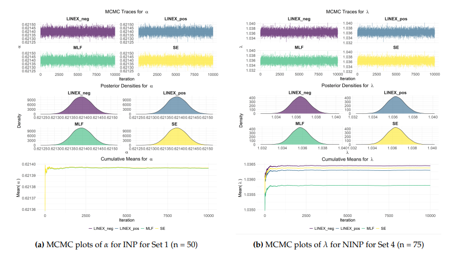
Figure 4 illustrates the MCMC diagnostics for estimating the parameters of the STLLBTL distribution for Sets 1 and 4, with sample sizes of 50 and 75, respectively, under both symmetric and asymmetric loss functions based on 10,000 replications. The trace plots indicate that the generated Markov chains fluctuate around stable values without any apparent trend, suggesting good mixing behavior. The posterior density plots appear approximately unimodal and symmetric, indicating well-defined posterior distributions. In addition, the cumulative mean plots stabilize rapidly as the number of iterations increases, confirming the convergence of the chains.
This section highlights the efficiency of the STLLBTL distribution when compared with other competing models, namely the sine inverted Weibull (SIW), inverse Lomax (IL), sine Frechet (SF), inverse power Lindley (IPL), and LBTL distributions. The comparison is carried out through two applications, each based on a real dataset. The ML method is employed to estimate the parameters of all competing distributions as well as the STLLBTL distribution. In addition, Bayesian estimation is applied to the STLLBTL distribution under different loss functions, including SE, LINEX with \(\tau=(-0.5,0.5)\), and MLF. To evaluate the goodness of fit, nine criteria are considered: minimum log-likelihood (\(-\log L\)), Akaike information criterion \((AIC)\), Bayesian information criterion \((BIC)\), consistent Akaike information criterion \((CAIC)\), Hannan-Quinn information criterion \((HQIC)\), Kolmogorov-Smirnov test \((KS)\), Anderson-Darling statistic \((AD)\), Cramer-von Mises statistic \((CvM)\), and p-value (\(P\)). The best-fitting distribution is identified as the one that achieves the smallest values for all criteria, with a high P-value.
AIC, BIC, CAIC, and HQIC are defined by: \(AIC=2p-2\log L, BIC=p\log n -2\log L, CAIC=-2\log L+p(\log n+1), HQIC=2p\log(\log n)-2\log L,\) where \(n\) is the number of observations, \(p\) is the number of parameters, and \(L\) is the maximum value of the likelihood function for a fitted model.
The first dataset represents a COVID-19 data belong to The United Kingdom of 60 days, from 1 December 2020 to 29 January 2021. These data were used by Almetwally [38].
0.1292, 0.3805, 0.4049, 0.2564, 0.3091, 0.2413, 0.1390, 0.1127, 0.3547, 0.3126, 0.2991, 0.2428, 0.2942, 0.0807, 0.1285, 0.2775, 0.3311, 0.2825, 0.2559, 0.2756, 0.1652, 0.1072, 0.3383, 0.3575, 0.2708, 0.2649, 0.0961, 0.1565, 0.1580, 0.1981, 0.4154, 0.3990, 0.2483, 0.1762, 0.1760, 0.1543, 0.3238, 0.3771, 0.4132, 0.4602, 0.3523, 0.1882, 0.1742, 0.4033, 0.4999, 0.3930, 0.3963, 0.3960, 0.2029, 0.1791, 0.4768, 0.5331, 0.3739, 0.4015, 0.3828, 0.1718, 0.1657, 0.4542, 0.4772, 0.3402.
The second dataset shows the United Kingdom COVID-19 mortality rates over a 28-day period (1 January 2022 to 28 January 2022). These data were used by Fayomi et al. [39].
0.1484, 0.1174, 0.0522, 0.0296, 0.0339, 0.2274, 0.1555, 0.1530, 0.2079, 0.0640, 0.1407, 0.2463, 0.2569, 0.2150, 0.1723, 0.1823, 0.1807, 0.1823, 0.2736, 0.2228, 0.2036, 0.1767, 0.1814, 0.1361, 0.1620, 0.2639, 0.2067, 0.2008.
Tables 6 and 7 present MLEs and BEs along with their corresponding precision measures, where standard errors (SErs) are associated with the MLEs and posterior standard deviations (PSDs) are associated with the BEs. Additionally, the confidence intervals (CIs) for the MLEs and credible intervals (CRIs) for the BEs are reported, with the remark that the BEs are computed only for the STLLBTL distribution under different loss functions, namely SE, LINEX with (\(\tau = -0.5, 0.5\)), and MLF using hyper-parameters \(\Big(a_{i}, b_{i}=0.0001, i=1, 2\Big)\), and are denoted as \(\Big(STLLBTL_{(SE)}, STLLBTL_{(LINEX-)}, STLLBTL_{(LINEX+)}, STLLBTL_{(MLF)}\Big)\).
| Distribution | \(\hat{\alpha}\) | \(\hat{\lambda}\) |
\(SEr (\hat{\alpha})\)/
\(PSD (\hat{\alpha})\) |
\(SEr (\hat{\lambda})\)/
\(PSD (\hat{\lambda})\) |
\(CI (\hat{\alpha})\)/
\(CRI (\hat{\alpha})\) |
\(CI (\hat{\lambda})\)/
\(CRI (\hat{\lambda})\) |
| STLLBTL | 5.073116 | 2.171101 | 0.871204 | 0.495321 | [3.365555, 6.780677] | [1.200271, 3.141931] |
| STLLBTL (SE) | 5.030404 | 1.681129 | 0.003323 | 0.002888 | [5.023738, 5.036812] | [1.675541, 1.686900] |
| STLLBTL (LINEX-) | 5.030475 | 1.681590 | 0.003317 | 0.002903 | [5.023836, 5.036874] | [1.675968, 1.687384] |
| STLLBTL (LINEX+) | 5.030332 | 1.680668 | 0.003330 | 0.002872 | [5.023656, 5.036744] | [1.675087, 1.686410] |
| STLLBTL (MLF) | 5.030290 | 1.678935 | 0.003334 | 0.002819 | [5.023595, 5.036705] | [1.673471, 1.684584] |
| SIW | 1.569392 | 0.127573 | 0.140169 | 0.031547 | [1.294661, 1.844124] | [0.065741, 0.189405] |
| IL | 31.749300 | 0.007467 | 17.894160 | 0.004210 | [-3.323253, 66.821856] | [-0.000785, 0.015721] |
| SF | 1.569321 | 0.269279 | 0.140208 | 0.018429 | [1.294512, 1.844130] | [0.233157, 0.305402] |
| IPL | 1.562612 | 0.172304 | 0.125530 | 0.038119 | [1.316573, 1.808651] | [0.097589, 0.247018] |
| LBTL | 7.874451 | – | 0.832932 | – | [6.241903, 9.506999] | – |
| Distribution | \(\hat{\alpha}\) | \(\hat{\lambda}\) |
\(SEr (\hat{\alpha})\)/
\(PSD (\hat{\alpha})\) |
\(SEr (\hat{\lambda})\)/
\(PSD (\hat{\lambda})\) |
\(CI (\hat{\alpha})\)/
\(CRI (\hat{\alpha})\) |
\(CI (\hat{\lambda})\)/
\(CRI (\hat{\lambda})\) |
| STLLBTL | 8.343901 | 1.871987 | 1.385674 | 0.519170 | – | – |
| STLLBTL (SE) | 8.319945 | 1.236894 | 0.003388 | 0.002855 | [8.313187, 8.326490] | [1.231438, 1.242673] |
| STLLBTL (LINEX-) | 8.319969 | 1.237403 | 0.003384 | 0.002870 | [8.313226, 8.326511] | [1.231908, 1.243215] |
| STLLBTL (LINEX+) | 8.319921 | 1.236385 | 0.003392 | 0.002839 | [8.313148, 8.326461] | [1.230973, 1.242126] |
| STLLBTL (MLF) | 8.319922 | 1.233599 | 0.003392 | 0.002761 | [8.313149, 8.326462] | [1.228366, 1.239149] |
| SIW | 1.119603 | 0.127932 | 0.137119 | 0.044031 | – | – |
| IL | 16.700607 | 0.007665 | 13.750470 | 0.006494 | – | – |
| SF | 1.119646 | 0.159359 | 0.137165 | 0.021995 | – | – |
| IPL | 1.083743 | 0.184533 | 0.120970 | 0.056323 | – | – |
| LBTL | 13.226124 | – | 1.737062 | – | – | – |
Based on Tables 6 and 7, when comparing BEs with MLEs, the BEs generally exhibit smaller PSDs, indicating higher precision. Moreover, the corresponding CRIs and CIs are relatively narrower in the case of the Bayesian approach, which further confirms the improved estimation accuracy. It is worth noting that, for the second dataset, only CRIs are reported since the sample size is small (\(n < 30\)), and hence CIs are not considered appropriate.
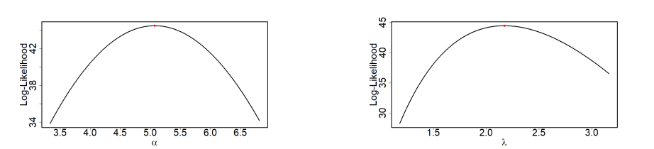
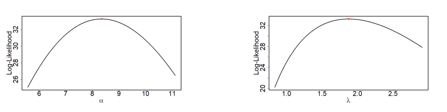
The profile log-likelihood of the STLLBTL distribution’s parameters, derived from the first and second data, is shown in Figures 5 and 6, respectively. They clearly illustrate how the profile log-likelihood behaves for the datasets. As shown in the figures, the parameters were obtained by maximizing the MLE of the STLLBTL distribution.
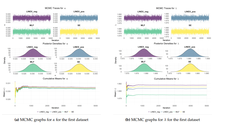
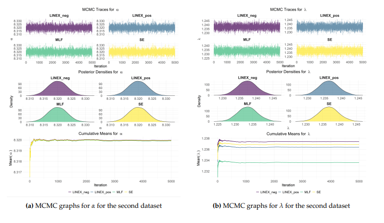
Figures 7 and 8 provide the MCMC diagnostic results for the estimated parameters \(\alpha\) and \(\lambda\) for the first and second data, respectively. The trace plots (top) indicate excellent mixing and stability of the chains. The posterior densities (middle) show the distribution of estimates under different loss functions, while the cumulative mean plots stabilize rapidly after the initial burn-in period, confirming the reliability of the obtained BEs. Overall, the stabilization across 5,000 iterations confirms the successful convergence of the algorithm. The M–H algorithm was implemented using a random-walk normal proposal distribution with covariance matrix \(\Sigma=\text{diag} (0.0001^2, 0.0001^2)\). The Markov chain was run for 5,000 iterations, and a burn-in period of 20% (1,000 iterations) was discarded to reduce the influence of initial values. The remaining 4,000 samples were retained for posterior inference. No thinning was applied, and all post-burn-in samples were used. The choice of the burn-in period was based on ensuring convergence of the Markov chain to its stationary distribution, as supported by trace plots and cumulative mean diagnostics. The average acceptance rate of the algorithm for the first data was 0.4999, while the average acceptance rate for the second data was 0.5000. These values indicate indicating an adequate balance between exploration of the parameter space and acceptance of proposed moves.
Tables 8 and 9 present the goodness-of-fit measures for the first and second data, including \(-\log L\), \(AIC\), \(BIC\), \(CAIC\), \(HQIC\), \(KS\), \(P\), \(AD\), and \(CvM\). Based on the obtained results, it is observed that the proposed STLLBTL model outperforms all competing models, including the baseline LBTL model, in terms of all goodness-of-fit criteria. This improvement can be attributed to the additional transformation structure, which increases the flexibility of the proposed model.
| Distribution | \(-\log L\) | \(AIC\) | \(BIC\) | \(CAIC\) | \(HQIC\) | \(KS\) | \(\mathbf{P}\) | \(AD\) | \(CvM\) |
|---|---|---|---|---|---|---|---|---|---|
| STLLBTL | -44.469 | -84.938 | -80.749 | -84.728 | -83.300 | 0.09575 | 0.60697 | 0.14575 | 0.84574 |
| SIW | -37.480 | -70.961 | -66.772 | -70.751 | -69.323 | 0.12746 | 0.26094 | 0.31658 | 1.81852 |
| IL | -12.713 | -21.426 | -17.237 | -21.215 | -19.787 | 0.35882 | 0.00000 | 0.29602 | 1.69630 |
| SF | -37.480 | -70.961 | -66.772 | -70.751 | -69.323 | 0.12746 | 0.26097 | 0.31658 | 1.81849 |
| IPL | -34.456 | -64.913 | -60.725 | -64.703 | -63.275 | 0.14749 | 0.13275 | 0.38124 | 2.19338 |
| LBTL | -28.631 | -55.263 | -53.169 | -55.194 | -54.444 | 0.17894 | 0.03752 | 0.17301 | 0.99141 |
| Distribution | \(-\log L\) | \(AIC\) | \(BIC\) | \(CAIC\) | \(HQIC\) | \(KS\) | \(\mathbf{P}\) | \(AD\) | \(CvM\) |
|---|---|---|---|---|---|---|---|---|---|
| STLLBTL | -33.271 | -62.542 | -59.877 | -62.062 | -61.727 | 0.19313 | 0.24721 | 0.27166 | 1.63124 |
| SIW | -24.507 | -45.015 | -42.350 | -44.535 | -44.200 | 0.27996 | 0.02482 | 0.59776 | 3.24693 |
| IL | -18.433 | -32.866 | -30.201 | -32.386 | -32.051 | 0.36962 | 0.00095 | 0.60322 | 3.27473 |
| SF | -24.507 | -45.015 | -42.350 | -44.535 | -44.200 | 0.27996 | 0.02482 | 0.59776 | 3.24696 |
| IPL | -22.126 | -40.252 | -37.588 | -39.772 | -39.438 | 0.29533 | 0.01513 | 0.67419 | 3.60923 |
| LBTL | -27.378 | -52.757 | -51.425 | -52.603 | -52.350 | 0.30427 | 0.01120 | 0.32936 | 1.93209 |
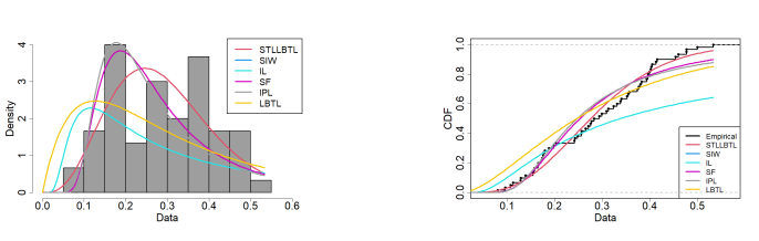
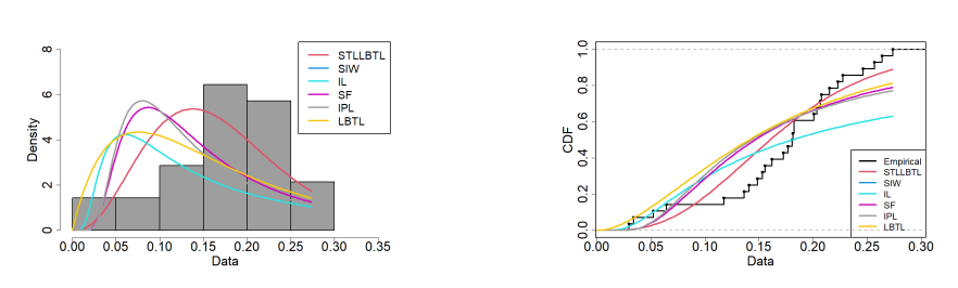
Figures 9 and 10 show the empirical PDF (EPDF) and empirical CDF (ECDF) of the STLLBTL distribution, alongside competing distributions, based on the first and second data, respectively. The comparison reveals that the STLLBTL distribution is the best in fitting the data among the considered distributions, as evident from both the EPDF and ECDF plots. This highlights the superior capability of the STLLBTL distribution in modeling the datasets.
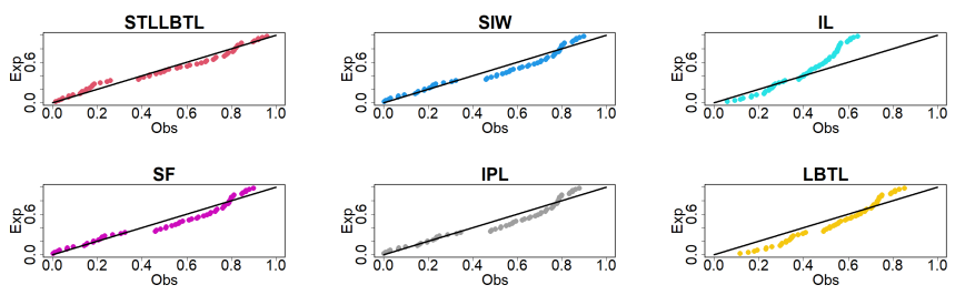
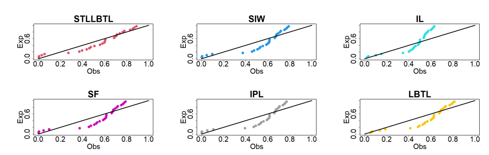
Figures 11 and 12 display the probability-probability (PP) plots for the competing distributions for the first and second data, respectively. These plots reveals that the STLLBTL distribution fits the datasets well.
In this study, a new two-parameter distribution called the STLLBTL distribution was introduced and investigated. Owing to its two shape parameters, the proposed model offers considerable flexibility, allowing it to accommodate various data behaviors and distributional shapes. Several important statistical properties were derived, including the survival function, hazard rate, reversed hazard rate, quantile function, moments, incomplete moments, as well as Renyi and Tsallis entropy measures. These properties highlight the theoretical richness and practical relevance of the proposed model. The model parameters were estimated using both maximum likelihood and Bayesian approaches under different loss functions, namely SE, LINEX, and MLF. A comprehensive Monte Carlo simulation study was conducted to assess the performance of the proposed estimators. The simulation results showed the expected trend, where the accuracy of both maximum likelihood and Bayesian estimates improves as the sample size increases. Overall, Bayesian estimates consistently outperformed maximum likelihood estimators across all considered scenarios. The practical applicability of the STLLBTL distribution was further demonstrated through two real data analyses, where it provided superior goodness-of-fit performance compared to competing models, as evidenced by lower information criteria values and higher P-values. These findings indicate that the STLLBTL distribution represents a flexible and effective modeling tool with distinctive characteristics suitable for real-life applications.
The study’s conceptualization and design were undertaken by [Amal S. Hassan], [Baria A. Helmy] and [Walaa A. Khamees], who were also responsible for data collection and analysis. The initial draft of the manuscript was composed by [Amal S. Hassan], [Baria A. Helmy] and [Walaa A. Khamees], and feedback on earlier versions was provided by [Amal S. Hassan], [Baria A. Helmy], [Walaa A. Khamees] and [Ahmed K. El koly]. All authors participated in the review and approval of the final manuscript.
The authors declare no conflict of interest.
All data required for this research is included within this paper.
No funding is available for this research.
We sincerely thank the editor and reviewers for their time and effort in handling this manuscript, and we appreciate their contribution to enhancing the quality of this paper.