
In recent years, fractional-order calculus has emerged as a significant branch of applied research. Since many physical and engineering systems inherently exhibit memory effects, fractional-order models provide an essential framework for accurately describing their dynamics [1– 4]. Extending integer-order calculus, fractional differential equations account for derivatives and integrals of arbitrary order, with the unique capability of capturing long-term memory phenomena [6– 8]. Furthermore, fractional-order chaotic systems have become a central topic in nonlinear dynamics, offering novel approaches for modeling, controlling, and synchronizing generalized dynamical systems [11– 13]. More recently, fractional calculus has been applied in financial markets, where economic and financial processes, characterized by strong nonlinearities and subjectivity, cannot be fully represented by integer-order models. In this context, exploiting bifurcation and chaos in fractional nonlinear dynamics is of particular importance [14– 16]. Compared with integer-order systems, fractional-order chaotic systems exhibit richer and more complex behaviors[17– 20]. Consequently, they have attracted considerable attention for both theoretical and practical applications, including secure communication, random signal generation, and cryptography [21– 24]. Alongside fractional dynamics, many nonlinear systems display multistability, where multiple attractors coexist under different initial conditions. Recent studies have linked this phenomenon closely to hidden attractors [25]. Several works have reported such behaviors, including three-dimensional chaotic systems with multiple attractors and circuit realizations [26], as well as four-dimensional systems with plane equilibria and coexisting attractors [27]. Other four-dimensional systems have been shown to generate chaotic or hyperchaotic attractors under conditions such as the absence of equilibria, the presence of a continuum of equilibria, or unstable equilibria, thereby revealing multistability among distinct attractors [28– 30]. Examples also include the Lü system, which exhibits periodic, chaotic, and point attractors depending on initial conditions [5], and systems such as a four-dimensional chaotic laser model [9], a cyclically symmetric chaotic system[10], and a memristor-based chaotic system [31].
Additionally, Particular attention has been given to four-dimensional fractional-order chaotic systems, which not only enrich the dynamical complexity of the underlying models but also enable the coexistence of multiple attractors, hidden dynamics, and novel bifurcation structures [32– 38]. This system’s innovation is in its capacity to produce numerous coexisting attractors for varying initial conditions and fractional orders, establishing a novel framework for investigating multistable dynamics in higher-dimensional fractional-order systems.
Unlike existing studies that merely extend known multi-wing systems to the fractional-order framework, this work introduces a novel four-dimensional nonlinear system whose structure intrinsically supports two-wing and four-wing attractors. The proposed fractional-order formulation reveals dynamical behaviors that do not appear in the integer-order case, including the emergence of hyperchaos induced by the fractional order and the coexistence of multiple attractors under identical system parameters. Moreover, a systematic Hopf bifurcation analysis is carried out in the fractional-order setting, where the fractional order acts as a bifurcation parameter, an aspect that has not been investigated for the corresponding integer-order system. The paper further presents a detailed study of chaos–hyperchaos transitions governed by the fractional order, supported by Lyapunov exponent analysis and phase-space diagnostics. These results demonstrate that fractionalization introduces fundamentally new dynamical mechanisms beyond a straightforward extension of the integer-order model.
We organize the sections of this work as follows: §2 presents an overview of fractional calculus, basic concepts, and further information on the stability of fractional dynamic systems. The fractional-order system investigated in this paper is introduced in §3. The Hopf bifurcation at equilibrium points is examined in §4. §5 investigates chaotic dynamics, such as self-excited attractors, coexisting attractors associated with multistability, and the hyperchaotic attractors of the fractional-order system. The comparison with the corresponding integer-order model is presented in §6. The main conclusions of the research are summarized in §7.
In this section, we introduce the essential concepts, definitions, and stability conditions of fractional-order systems that are required throughout the paper. Several standard definitions are used in fractional calculus in the literature; see [39, 40]. We summarize those most relevant to our study.
The fractional calculus extends the concept of classical integer-order integration and differentiation to non-integer orders. In this work, we adopt the standard definitions based on the Riemann–Liouville fractional integral and the Caputo fractional derivative[39, 41].
Definition 1. ([39, 41]). The Riemann–Liouville fractional integral of order \(\omega>0\) for a function \(f(t)\) is defined as \[\left(I_{t_0}^{\omega} f\right)(t) = \frac{1}{\Gamma(\omega)} \int_{t_0}^{t} (t-\tau)^{\omega-1} f(\tau)\, d\tau, \quad \omega>0, \tag{1}\] where \(\Gamma(\cdot)\) denotes the Gamma function.
Definition 2. ([39, 41]). The Caputo fractional derivative of order \(\omega\), with \(m-1<\omega<m\) and \(m\in\mathbb{N}\), is defined as \[\left( {}^{C}D_{t_0}^{\omega} f \right)(t) = \frac{1}{\Gamma(m-\omega)} \int_{t_0}^{t} (t-\tau)^{m-\omega-1} f^{(m)}(\tau)\, d\tau. \tag{2}\]
The fractional integral operator \(I_{t_0}^{\omega}\) possesses the following three fundamental properties: \[ {}_{t_0}I_t^\omega (t – t_0)^\sigma = \frac{\Gamma(\sigma + 1)}{\Gamma(\sigma + 1 + \omega)} (t – t_0)^{\sigma + \omega},\ \tag{3}\] \[{}_{t_0}I_t^\omega W = \frac{W}{\Gamma(\omega + 1)} (t – t_0)^\omega,\ \tag{4}\] \[{}_{t_0}I_t^\omega {}_{t_0}I_t^v g(t) = {}_{t_0}I_t^{\omega + v} g(t). \tag{5}\]
In this context, \(t_0\) represents the initial time, \(\omega \geq 0\), \(v \geq 0\), \(\sigma > -1\), and \(W\) is a real-valued constant.
The fractional-order dynamical system considered in this paper is solved numerically using the Adams–Bashforth–Moulton (ABM) predictor–corrector scheme for Caputo fractional derivative, which was first introduced by Diethelm et al. in [42]. This method is widely used for fractional-order systems with initial value problems and provides reliable numerical approximations.
We consider a general \(n\)-dimensional fractional-order system written in vector form as \[\begin{aligned} \label{7} \left\{ \begin{aligned} &\ {_{t_0}^{C}}D_{t}^\omega y(t) = g(t, y(t)), \quad 0 \leq t \leq T, \\ &\ y^{l}(0) = y_0^{(l)}, \quad l = 0,1, \dots, \lceil \omega \rceil -1, \ \ m-1< \omega < m, \ m \in \mathbb{N}. \end{aligned} \right. \end{aligned} \tag{6}\]
This equation corresponds to the Volterra integral equation (see Section 2 in [42]): \[\begin{aligned} \label{2} y(t) = \sum_{l=0}^{\lceil \omega \rceil -1} y_0^{(l)} \frac{ t^l}{l!} + \frac{1}{\Gamma(\omega)} \int_{0}^{t} (t – \psi)^{(\omega-1)} g(\psi, y(\psi)) d\psi. \end{aligned} \tag{7}\]
The time interval \([0,T]\) is discretized into \(m\) uniform subintervals of size \(h = T/m\), with grid points \(t_\epsilon = \epsilon h, \ \epsilon = 0, 1, \dots, m\).
In this work, the full-memory formulation of the ABM method is employed; hence, all previous states contribute to the numerical approximation, and no short-memory approximation is used.
The corrector method for equation (7) can be described as follows (see[42] pages 3–6 for full details): \[\begin{aligned} y_h (t_{m+1}) &= \sum_{l=0}^{\lceil \omega \rceil -1} y_0^{(l)} \frac{t_{m+1}^l}{l!} + \frac{h^\omega}{\Gamma(\omega+2)} g(t_{m+1}, y_h^p (t_{m+1})) + \frac{h^\omega}{\Gamma(\omega+2)} \sum_{\epsilon=0}^{m} \phi_{\epsilon,m+1} g (t_\epsilon, y_h (t_\epsilon)), \end{aligned} \tag{8}\] where the predictor values \(y_h(t_{m+1})\) are computed using the approach presented in [42], \[\begin{aligned} y_h^p (t_{m+1}) &= \sum_{l=0}^{\lceil \omega \rceil -1} y_0^{(l)} \frac{t_{m+1}^l}{l!} + \frac{1}{\Gamma(\omega)} \sum_{\epsilon=0}^{m} \Omega_{\epsilon,m+1} g(t_\epsilon, y_h (t_\epsilon)), \end{aligned} \tag{9}\] where the weights \(\phi_{\epsilon,m+1}\) and \(\Omega_{\epsilon,m+1}\), as defined in [42], are given by the following formulas: \[\begin{aligned} \phi_{\epsilon,m+1} = \begin{cases} m^{\omega+1} – (m-\omega) (m+1)^\omega, & \epsilon = 0, \\ (m-\epsilon+2)^{\omega+1} + (m-\epsilon)^{\omega+1} – 2(m-\epsilon+1)^{\omega+1}, & 1 \leq \epsilon \leq m, \\ 1, & \epsilon = m+1, \end{cases} \end{aligned} \tag{10}\] and \[\begin{aligned} \Omega_{\epsilon,m+1} = \frac{h^\omega}{\omega} \big( (m+1-\epsilon)^\omega – (m-\epsilon)^\omega \big), \quad 1 \leq \epsilon \leq m. \end{aligned} \tag{11}\]
In all numerical simulations, the system is integrated over a sufficiently long time interval, a sufficiently small step size \(h\) is chosen to ensure numerical accuracy, and the phase portraits are obtained from the resulting trajectories. While transient dynamics are not analyzed explicitly, the plotted trajectories correspond to the long-term behavior of the system and are sufficient to identify the qualitative nature of the observed attractors.
It is worth emphasizing that the above formulation and numerical scheme are valid for general fractional orders satisfying \(m-1<\omega<m\), and are not restricted to the case \(\omega\in(0,1)\).
This subsection addresses the requisite condition for the stability of a generic fractional-order system. Initially, the following fractional-order differential system is considered. \[\label{13}\begin{cases} {_{t_0}^{C}}D_{t}^{\omega_i}y_j(t) = g_j(y_1(t), y_2(t), \ldots, y_m(t),t), \\ y_i(0)=y_j, \quad \text{for} \ j=1,…,m. \end{cases} \tag{12}\]
The system structure and associated stability condition are discussed in[43– 45]. The Jacobian matrix structure of the fractional-order system (12) assessed at the equilibrium point \(E^* = (y_1^*, y_2^*, \ldots, y_m^*)\) is determined as \[J = \Big[ \frac{\partial g_i}{\partial y_j}\Big], \ \text{for} \ \ i,j=1,…,m. \tag{13}\]
Definition 3. ([46]). Consider the fractional-order system (12), where the current state vector is written as \(\mathbf{y} = (y_1, y_2, \dots, y_m)^T\), and the vector that shows the orders of the fractional derivatives is \(\mathbf{\omega} = (\omega_1, \omega_2, \dots, \omega_m)^T\), with each \(\omega_j > 0\), for \(j = 1, \ldots, m\). When all of the derivatives’ orders are the same, the system is known as a commensurate-order system, meaning \((\omega_1 = \omega_2 = \dots = \omega_m)\); if they are not the same, it is referred to as an incommensurate-order system.
Definition 4. ([47]). A point \(E^*\) is defined as an equilibrium point of system (12) exactly when it satisfies the condition \(g_j(t, E^*) = 0; \text{for} \ j = 1,…,m.\)
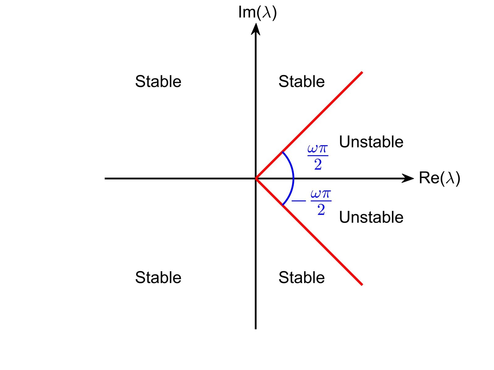
Theorem 1. ([48]). Considering the commensurate fractional-order system (12), the equilibrium point \(E^*\) is locally asymptotically stable if each eigenvalue \(\lambda_j\) of the Jacobian matrix \(J(E^*)\) possesses angles exceeding \(\frac{\omega \pi}{2}\), precisely \(|\arg(\lambda_j)| > \frac{\omega \pi}{2}\). If the previous requirement is not satisfied, the equilibrium point \(E^*\) is unstable.
From the above theorem, Figure 1 depicts the stability zone of the fractional-order system (12) for \(0<\omega<1\).
This section introduces the system that we will analyze in subsequent sections. An integer-order version of this model, which was proposed by Huang et al. in [49], shows bifurcation phenomena and chaotic dynamics that are controlled by the following four equations: \[\begin{aligned} \label{15} \left\{ \begin{aligned} \dot{x} &= py – px, \\ \dot{y} &= xz + w, \\ \dot{z} &= k – xy, \\ \dot{w} &= yz – vw , \end{aligned} \right. \end{aligned} \tag{14}\] where \((p, k, v) \in \mathbb{R}_{+}^{3}\) are parameterics of the system and \(x, y, z\), and \(w\) denote state variables.
Throughout this work, all parameters are assumed to be strictly positive to ensure the physical meaningfulness of the model and to guarantee the existence of nontrivial equilibrium points. This admissible parameter set is used consistently in the stability, bifurcation, and numerical analyses presented in the subsequent sections.
The admissible parameter domain defines the range over which the model is well posed, whereas Hopf bifurcation occurs only for specific parameter values within this domain, as determined by the eigenvalue conditions of the Jacobian matrix.
Applying Definition 2, the commensurate Caputo fractional-order system (14) can be express by \[\begin{aligned} \label{16} \left\{ \begin{aligned} {_{t_0}^{C}}D_{t}^\omega x &= py – px, \\ {_{t_0}^{C}}D_{t}^\omega y &= xz + w, \\ {_{t_0}^{C}}D_{t}^\omega z &= k – xy, \\ {_{t_0}^{C}}D_{t}^\omega w &= yz – vw, \end{aligned} \right. \end{aligned} \tag{15}\] where \(0<\omega<1\) and the initial conditions are given by \((x(0), y(0), z(0), w(0))=(x_0,y_0, z_0, w_0)\).
We note that under standard conditions, specifically when the right-hand side of the system is continuous and satisfies a Lipschitz condition, the existence and uniqueness of solutions to the fractional-order system are guaranteed [39, 40]. These conditions are fulfilled in our scenario, ensuring that the fractional-order initial value problem is well-posed.
By using Definition 4, \({_{t_0}^{C}}D_{t}^\omega x = {_{t_0}^{C}}D_{t}^\omega y = {_{t_0}^{C}}D_{t}^\omega z ={_{t_0}^{C}}D_{t}^\omega w= 0\), the equilibrium points of the fractional-order system (15) can be determined via the solution of the following calculation: \[\begin{aligned} \label{17} \left\{ \begin{aligned} py – px=0, \\ xz + w=0, \\ k – xy=0, \\ yz – vw=0. \end{aligned} \right. \end{aligned} \tag{16}\]
According to [49], two equilibrium points are obtained: \(E_{1,2}=(\pm \sqrt{k},\pm \sqrt{k},0,0)\).
The equilibrium points are real and exist when \(k > 0\), resulting in two equilibrium points: \((\pm \sqrt{k},\pm \sqrt{k},0,0)\). The Jacobian matrix based at the equilibrium point \(E=(x,y,z,w)\) is \[\begin{aligned} J_E=\left[\begin{array}{cccc} -p & p & 0 & 0 \\ z & 0 & x & 1 \\ -y & -x & 0 & 0 \\ 0 & z & y & -v \end{array}\right], \end{aligned} \tag{17}\] and the corresponding characteristic polynomial is of the form \[\begin{aligned} \label{char} P_E(\lambda)=\lambda^4 + \kappa \lambda^3 + \eta \lambda^2 +\Upsilon \lambda + \Delta, \end{aligned} \tag{18}\] where \(\lambda\) denotes the eigenvalue of the system, and \[\begin{aligned} \kappa&= v + p,\\ \eta &= pv – pz + x^2 – z,\\ \Upsilon &= -pvz + px^2 + pxy + vx^2 – pz + xy, \\ \Delta &= pvx^2 + pvxy + pxy + py^2. \end{aligned}\]
By selecting appropriate parameter values, the stability regions of the system can be identified and the occurrence of Hopf bifurcation can be demonstrated. The stability of the equilibrium points and the emergence of Hopf bifurcation are determined by the roots of the characteristic polynomial (18). Since the accuracy of the stability analysis depends critically on the correctness of the Jacobian matrix and its characteristic polynomial, a detailed and verifiable derivation of the Jacobian matrix and the coefficients of the characteristic polynomial is provided in Appendix A.
Notably, in integer-order system (14), Hopf bifurcation has not been studied. Under certain fractional order conditions, the analysis verifies that the fractional-order system transitions from stable to unstable dynamics. Thus, the system (15) displays chaotic behavior. These findings demonstrate the fundamental importance of a fractional order in the system’s dynamics. Further details will be provided in the subsequent sections.
In integer-order dynamical systems, a Hopf bifurcation occurs when a pair of complex conjugate eigenvalues of the Jacobian matrix crosses the imaginary axis, leading to a change in the stability of an equilibrium point. However, this classical interpretation does not directly apply to fractional-order systems.
For commensurate fractional-order systems of order \(\omega \in (0,1)\), local asymptotic stability is governed by the angle condition \[\begin{aligned} |\arg(\lambda_j)|>\frac{\omega \pi}{2}, \ \ j=1,…,4. \end{aligned}\] where \(\lambda_j\) are the eigenvalues of the Jacobian matrix. Consequently, variations in the fractional order \(\omega\) can alter the stability of an equilibrium point even when the eigenvalues themselves remain unchanged.
In this work, we distinguish between (i) stability changes induced by varying the fractional order \(\omega\), and (ii) classical Hopf bifurcation caused by changes in system parameters that modify the eigenvalues. Following the fractional Hopf bifurcation criterion proposed by Ranchao Wu and Xiang Li [50], the fractional order \(\omega\) is treated as the bifurcation parameter.
In this part, we focus on the long-term behavior of trajectories, disregarding transient states. Although the limit cycle that emerges from a Hopf bifurcation does not solve the fractional-order system exactly, it serves as an attractor for nearby solutions. Several studies in fractional order systems have investigated the presence of Hopf bifurcation[50, 51]. We define the function \(g\) with respect to \(\omega\) as follows: \[\begin{aligned} g(\omega) = \frac{\omega \pi}{2} – \min_{1 \leq j \leq 4} \left| \arg(\lambda_j) \right|. \end{aligned} \tag{19}\]
In this context, \(\omega\) represents the fractional order, which serves as the bifurcation parameter of the given system, while the \(\lambda_j\)’s denote the eigenvalues of the Jacobian matrix of the fractional-order system (15). Additionally, an equilibrium point is locally asymptotically stable if \(g(\omega)\ <0\) and unstable when \(g(\omega) >0\). The subsequent theorem is necessary to examine the Hopf bifurcation of fractional-order differential systems.
Theorem 2. ([50]) (Criteria for the emergence of Hopf bifurcation). The fractional-order system (15) shows a Hopf bifurcation at the equilibrium points \(E_{1,2}\) when the bifurcation parameter \(\omega\) cross the critical threshold \(\omega^* \in (0,1)\), provided that the following criteria are satisfied:
The Jacobian matrix of system (15) at the equilibrium point includes two complex conjugate eigenvalues \(\lambda_{1,2} = \rho \pm i \mu\), where \(\rho > 0\) and \(\mu \neq 0\), in addition to two negative real eigenvalues \(\lambda_3\) and \(\lambda_4\).
\(g(\omega^*) = 0 , \ (\omega^* = \frac{2}{\pi}|arg(\lambda_{1,2})|)\),
\(\left. \frac{d[g(\omega)]}{d\omega} \right|_{\omega=\omega^*} \neq 0\), (Condition of transversality).
So, the equilibrium point is locally asymptotically stable for \(\omega \in (0, \omega^\ast )\) and is unstable when \(\omega \in (\omega^\ast,1)\). Therefore, the system undergoes a fractional Hopf bifurcation at the critical fractional order \(\omega = \omega^\ast\).
Remark 1. In the present analysis, the bifurcation parameter is the fractional order \(\omega\), whereas the eigenvalues of the Jacobian matrix depend only on the system parameters and remain independent of \(\omega\). Consequently, the function \(g(\omega)\) varies linearly with respect to \(\omega\), and the transversality condition \[\begin{aligned} \left. \frac{d[g(\omega)]}{d\omega} \right|_{\omega=\omega^*} \neq 0, \end{aligned}\] is automatically satisfied, since \(\frac{d[g(\omega)]}{d\omega} = \frac{\pi}{2}> 0\). This behavior is consistent with the fractional Hopf bifurcation criterion proposed by Wu and Xiang Li [50].
Unlike integer-order systems, the oscillatory behavior emerging at a fractional Hopf bifurcation does not correspond to a classical periodic solution of the system. Instead, the system exhibits an attracting oscillatory limit set that governs the long-term behavior of nearby trajectories. Such fractional-order oscillations have been widely reported in the literature and are characteristic of Hopf bifurcation induced by variations in the fractional order \(\omega\) [50, 51].
In the following subsection, we’ll determine the fractional order \(\omega\) using Theorem 1 and utilize numerical simulations, as presented in §2.2, to demonstrate that our system exhibits rich, complex dynamics. We will also determine the range of stability and investigate the Hopf bifurcation for the chosen parameters at both equilibrium points, including the related fractional order at which it occurs.
This subsection performs a numerical stability analysis to investigate that our system undergoes a Hopf bifurcation and to determine the existence of both equilibrium points. These numerical calculations aim to demonstrate the impact of parameter values and changes in the derivative order \(\omega\) on the dynamic behaviour of the fractional-order system (15). Without loss of generality, the parameters \(p=14,\ k=1\), and \(v=4\) are considered. Using the Maple program for the following calculation, the equilibrium points calculated with these parameters are \(E_{1,2}=( \pm 1, \pm 1, 0, 0)\). The Jacobian matrix of the system, assessed at \(E_{1,2}\) is: \[\begin{aligned} J_{E_{1,2}}=\left[\begin{array}{cccc} -14 & 14 & 0 & 0 \\ 0 & 0 & \pm 1 & 1 \\ \pm 1 & \pm 1 & 0 & 0 \\ 0 & 0 & \pm 1 & -4 \end{array}\right]. \end{aligned} \tag{20}\]
Both equilibrium points \(E_{1,2}\) possess identical characteristic polynomials, expressed as \[\begin{aligned} PE_{1,2}(\lambda)=\lambda^4+ 18\lambda^3+ 57\lambda^2 + 33 \lambda + 140. \end{aligned}\]
Let \(\mid \lambda I-
J_{E_{1,2}}\mid\), then the eigenvalues are given as \(\lambda_{1,2}=0.0938 \pm 1.5509 i,\ \lambda_3 =
-4.1242\),
and \(\lambda_4 = -14.063\). By Theorem
1, the equilibrium points
\(E_{1,2}\) are locally asymptotically
stable where \[\begin{aligned}
|arg(\lambda_{1,2})|&=tan^{-1}\Big(\frac{1.5509}{0.0938}\Big)=1.5104>\frac{\omega
\pi}{2},\ \ \ 0<\omega<\omega^*<1,\\
&\text{and unstable when}\ \ 0<\omega^*<\omega<1.
\end{aligned}\]
From condition 2 in Theorem 2, the critical value parameter \(\omega^*\) of bifurcation is follows: \[\begin{aligned} \omega^*=\frac{2}{\pi}tan^{-1}\Big(\frac{1.5509}{0.0938}\Big) \approx 0.9615, \ \ \left. \frac{d[f(\omega)]}{d \omega} \right|_{\omega=\omega^*}=\frac{\pi}{2} \neq 0. \end{aligned}\]
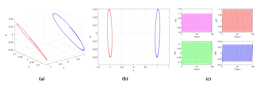
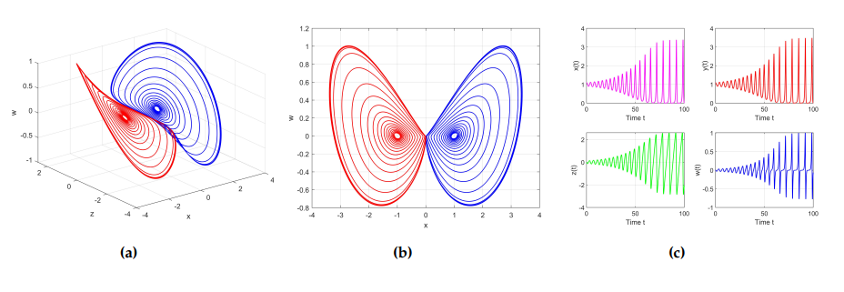
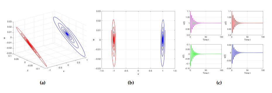
A Hopf bifurcation is confirmed to occur at both equilibrium points \(E_{1,2}\) whenever the bifurcation parameter \(\omega\) crosses the critical threshold \(\omega^*\), i.e., \(\omega=\omega^*=0.9615\) (see Figure 2). If \(\omega\) is greater than \(\omega^*\), then both equilibrium points \(E_{1,2}\) are unstable. For instance, when we set \(\omega = 0.98\), which is greater than \(\omega^*\), the equilibrium points \(E_{1,2}\) lose their stability (see Figure 3). However, both equilibrium points \(E_{1,2}\) are locally asymptotically stable if \(\omega\) is less than \(\omega^*\). In this example, we set \(\omega = 0.92\), which is less than \(\omega^* = 0.9615\); therefore, both equilibrium points \(E_{1,2}\) are locally asymptotically stable (see Figure 4). More details are presented in the next discussion subsection.
The numerical computations were carried out in an attempt to study the behavior of the fractional-order system dynamics with various fractional orders \(\omega \in (0.92, 1]\). As indicated in Figure 2, the phase space diagram and the corresponding time series exhibit limit cycles resulting from a Hopf bifurcation at both symmetric equilibrium points \(E_{1,2}\), which were analyzed using the predictor-corrector method and illustrated with MATLAB software. Simulations use initial conditions \((1.1,1.1,0.01,0.01)\) and a fractional order \(\omega=0.9615\). The blue trajectory corresponds to the solution around the first equilibrium point \(E_1=(1,1,0,0)\). In contrast, the red trajectory illustrates the limit cycle around the second equilibrium point \(E_2=(-1,-1,0,0)\), and these equilibrium points are numerically shown to be symmetric. The 3D phase space diagram \(xzw\)-space displays two visible, symmetrical limit cycles emanating from both equilibrium points \(E_{1,2}\), which represent ongoing oscillations resulting from a Hopf bifurcation, as shown in Figure 2a. Figure 2b shows a 2D projection onto the \(xw\)-plane. Additionally, in Figure 2c, the trajectories of \(x(t), y(t), z(t)\) and \(w(t)\) over time illustrate sustained oscillations caused by the Hopf bifurcation at \(\omega=\ 0.9615\).
Phase space diagrams and the corresponding time series for the fractional-order system with \(\omega=0.98\) and initial conditions \((1.1,1.1,0.01,0.01)\) are presented in Figure 3, illustrating instability at both equilibrium points \(E_{1,2}\). The 3D phase space diagram in the \(xzw\)-space shown in Figure 3a displays two unstable oscillatory trajectories that diverge from the equilibrium points \(E_{1,2}\). Figure 3b depicts the corresponding two-dimensional projection onto the \(xw\)-plane. Furthermore, the time evolutions of \(x(t),\ y(t),\ z(t)\) and \(w(t)\) indicate a departure from the equilibrium points and the emergence of unstable oscillatory dynamics. The trajectories remain bounded and evolve within a finite region of the phase space, as illustrated in Figure 3c.
In Figure 4, the phase space diagram and the corresponding time series for \(\omega = 0.92\) are displayed to illustrate local asymptotic stability at both symmetric equilibrium points \(E_{1,2}\) using the initial conditions \((1.1,1.1,0.01,0.01)\). Figure 4a shows the 3D phase space diagram where stable limit cycles converge towards both equilibrium points \(E_{1,2}\), indicating that they are locally stable over time. Additionally, the 2D projection onto the \(xw\)-plane is demonstrated in Figure 4b. Furthermore, Figure 4c confirms the local stable behavior by demonstrating the trajectories of \(x(t),\ y(t), \ z(t)\) and \(w(t)\) over time and the trajectories approaching both equilibrium points \(E_{1,2}\) as \(t\rightarrow \infty\).
In this part, we investigate the complex dynamical behaviors of the fractional-order system (15), including the emergence of chaos, the formation of self-excited attractors, and the coexistence of multiple attractors that lead to multistability, by assigning appropriate parameter values and defining an appropriate fractional order \(\omega\). To identify parameter regimes that may support chaotic dynamics in the fractional-order system (15), we employ a necessary instability criterion derived from the literature. This criterion does not by itself guarantee the existence of chaos, but it indicates parameter regions where chaotic attractors may arise. The actual presence of chaos is subsequently verified through numerical simulations, including phase portraits and Lyapunov exponent analysis.
Theorem 3. ([46, 52]). To demonstrate chaotic behavior in the fractional-order system (15), at least one eigenvalue \(\lambda = \rho \pm i \mu\), must stay in the unstable area. In other words, the presence of instability in the system is a key requirement for the persistence of chaos. Mathematically the chaotification condition is given by \[\begin{aligned} \omega \geq \frac{2}{\pi} \left( \tan^{-1} \left| \frac{\mu}{\rho} \right|\right), \end{aligned}\] where \(\omega\) is the fractional order and \(\lambda\) are the eigenvalues of the saddle-focus equilibrium point of index 2 in the fractional-order system (15).
In this paper, Theorem 3 provides a necessary instability condition for the persistence of complex dynamics in fractional-order systems. However, instability alone does not imply the existence of a chaotic attractor. Therefore, Theorem 3 is used only to delimit parameter regions where chaotic behavior may occur. The existence of chaos is confirmed numerically by means of phase portraits, time series, and Lyapunov exponent computations. In particular, we emphasize that linear instability or satisfaction of the angle condition is not equivalent to the existence of a chaotic attractor.
In accordance with standard definitions, an attractor is termed self-excited if its basin of attraction intersects a neighborhood of an unstable equilibrium point. In the present work, the observed attractors are self-excited, since they can be obtained by numerical integration starting from initial conditions chosen arbitrarily close to the unstable equilibrium points of the system. Furthermore, for fixed parameter values, different attractors are observed for different initial conditions, indicating the coexistence of multiple attractors. We do not claim the existence of hidden attractors in this study, as a detailed basin-of-attraction analysis is beyond the scope of the present work.
For all reported attractor types, including two-wing, four-wing, and coexisting attractors, the numerical diagnostics are computed using a consistent protocol. Specifically, phase portraits and Lyapunov exponents are obtained using the same fractional-order numerical scheme, identical parameter values, fixed integration time, and the same transient interval discarded prior to analysis. The Lyapunov spectra are calculated using the same algorithm and normalization procedure for all cases, ensuring a fair comparison between different dynamical regimes. Together, these diagnostics provide a consistent characterization of the system dynamics.
Although Poincaré sections are commonly used in integer-order systems, in this work the identification of chaotic and hyperchaotic dynamics is based on the combined use of phase-space projections and Lyapunov spectra, which are widely accepted diagnostic tools for fractional-order systems.
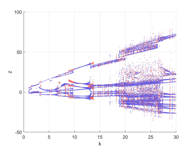
The parameters \(p=0.1\) and \(v=1\) are considered for the fractional-order system (15). We plot the bifurcation diagram of the \(z\)-peak in Figure 5 versus the control parameter \(k \in [1,30]\), with fractional derivative order \(\omega=0.96\). The diagram is obtained using the predictor–corrector method by employing two different sets of initial conditions: the forward initial condition \(X^+ = (2,2,2,2)\), shown in red, and the backward initial condition \(X^-= (-2,-2,-2,-2)\), shown in blue. The figure demonstrates that as parameter \(k\) increases, the system transitions between periodic and chaotic behaviors, reflecting the rich bifurcation structure and chaotic dynamics of the fractional-order model.
Let \(k = 26, \ p=0.1\) and \(v=1\). Under these parameters, we have two equilibrium points and given by \(E_{1,2}=(\pm \sqrt{26}, \pm \sqrt{26},0,0)\). The eigenvalues for these equilibrium points are \(\lambda_{1,2}=0.48732 \pm 5.2450i, \ \lambda_3= -0.19993\), and \(\lambda_4= -1.8747\). Therefore, \(E_{1,2}\) are unstable saddle-focus points equilibria of index \(2\), since they possess two nonzero positive real parts of complex eigenvalues and two other negative eigenvalues, which are precisely the type of points around which scroll attractors form in four-dimensional multiscroll chaotic systems[53]. Based on the Theorem 3, the condition necessary for the emergence of chaos is \[\begin{aligned} \omega \geq \frac{2}{\pi} \left( \tan^{-1} \left| \frac{5.2450}{0.48732} \right|\right)\approx 0.941. \end{aligned}\]
Therefore, the commensurate fractional order \(\omega\) must satisfy the \(\omega \geqslant 0.941\), in order to maintain the instability of the eigenvalue.
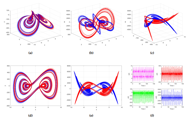
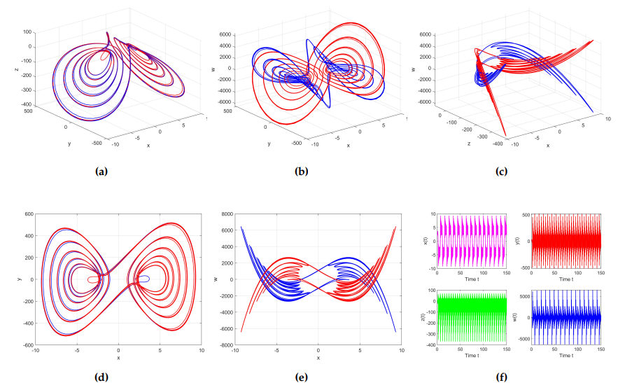
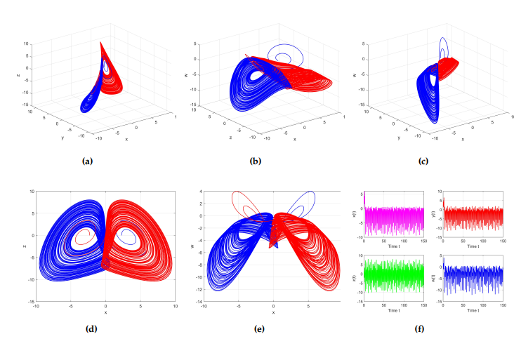
In this subsection, we generate self-excited chaotic phase portraits with two varying fractional orders \(\omega =0.96\) and \(\omega =0.99\), values to verify chaos in the system parameters (\(p=0.1, \ k=26,\ \text{and} \ v=1\)) selected in the previous subsection. Under these parameter values, the fractional-order system (15) exhibits chaotic behavior, as illustrated in Figures 6 and 7. Simulations are based on the same initial conditions \((2, 2, 2, 2)\), evaluated over the time interval \([0, 150]\). In these figures, we display the self-excited chaotic attractors of system (15), which were obtained using the numerical scheme for the predictor-corrector method. The 3D phase portraits in figures 6 and 7 display a two-wing and four-wing chaotic attractor, indicating trajectories exhibit a butterfly-like structure, which is typical of self-excited attractors around a pair of symmetric unstable equilibrium points. As the fractional order escalates from \(\omega=0.96\) to \(\omega=0.99\), the wing scrolls exhibit greater density and structure. Furthermore, Figures 6d and 7d in \(xy\)-plane show a classical Lorenz-type two-wing attractor. Also, Figures 6e and 7e in \(xw\)-plane illustrate a four-wing attractor, which indicates chaotic behavior of the system under the selected parameters and fractional order. Finally, Figures 6f and 7f provide the corresponding time series for \(x(t),\ y(t),\ z(t)\), and \(w(t)\) of these chaotic motions, where irregular oscillations confirm the presence of self-excited chaotic behavior. In particular, the structure of the wing scrolls is visible, with tighter loops and more intricate layering in Figure 7 compared to Figure 6. This research suggests that elevating the fractional order towards one results in enhanced dynamical behavior and complexity. The data indicate that the system consistently exhibits a chaotic attractor with geometric complexity and trajectory density escalating as \(\omega \rightarrow 1\).
In this subsection, Lyapunov exponents are employed to characterize the chaotic and hyperchaotic behavior of the fractional-order system (15). The computation is carried out using the algorithm proposed by Danca et al. [54], adapted to fractional-order systems. The original system is integrated using the fractional predictor–corrector method, and simultaneously, the associated variational equations are constructed from the Jacobian matrix of system (15).
The combined system consisting of the state equations and the variational equations is numerically integrated with the same step size \(h=0.006\). During the integration process, a QR (Gram–Schmidt) reorthonormalization procedure is applied at fixed time intervals to maintain numerical stability and orthogonality of the tangent vectors. The Lyapunov exponents are then obtained from the time-averaged logarithmic growth rates of these vectors after discarding an initial transient period.
This procedure allows reliable estimation of the full Lyapunov spectrum for the fractional-order system and is widely used in the literature for chaos analysis in fractional dynamical systems.
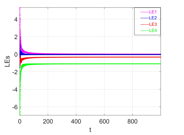
These exponents provide a fundamental tool for identifying chaos, particularly when at least one of them is positive, signifying that the system is completely unpredictable. For all numerical simulations, we fixed parameter values \(p= 0.1,\ k=26\), and \(v=1\), with initial conditions \((2,2,2,2)\). The dynamic behavior of the system includes calculating the four Lyapunov exponents, namely \(LE1,\ LE2,\ LE3\), and \(LE4\), as demonstrated in Figure 8. The Lyapunov exponents are determined for the time t from \(0\) to \(1000\) with a fractional order of \(\omega=0.96\), yielding values of \((LE1,\ LE2,\ LE3,\ LE4)=( 0.010, -0.0486, -0.3260, -1.0958)\), given in Table 1. The presence of a positive largest Lyapunov exponent \(LE1\) confirms the existence of chaotic dynamics in the fractional-order system (15). Furthermore, for all computed time horizons, the sum of the Lyapunov exponents remains negative. This indicates an overall contraction of nearby trajectories in the phase space, implying that the fractional-order system (15) is dissipative in the sense of Lyapunov stability. Combined with the presence of at least one positive Lyapunov exponent, this confirms the existence of chaotic dynamics in the system.
| Time | LE1 | LE2 | LE3 | LE4 |
|---|---|---|---|---|
| 50 | 0.149 | 0.0153 | -0.4548 | -1.1643 |
| 100 | 0.104 | -0.0500 | -0.3719 | -1.1398 |
| 150 | 0.056 | -0.0306 | -0.3654 | -1.1187 |
| 200 | 0.051 | -0.0423 | -0.3466 | -1.1208 |
| 250 | 0.037 | -0.0388 | -0.3516 | -1.1058 |
| 300 | 0.040 | -0.0502 | -0.3387 | -1.1097 |
| 350 | 0.035 | -0.0472 | -0.3392 | -1.1080 |
| 400 | 0.024 | -0.0491 | -0.3375 | -1.0970 |
| 450 | 0.027 | -0.0476 | -0.3344 | -1.1041 |
| 500 | 0.020 | -0.0503 | -0.3327 | -1.0966 |
| 550 | 0.019 | -0.0505 | -0.3307 | -1.0971 |
| 600 | 0.016 | -0.0516 | -0.3316 | -1.0931 |
| 650 | 0.011 | -0.0488 | -0.3287 | -1.0935 |
| 700 | 0.012 | -0.0488 | -0.3302 | -1.0929 |
| 750 | 0.011 | -0.0500 | -0.3287 | -1.0920 |
| 800 | 0.011 | -0.0480 | -0.3293 | -1.0935 |
| 850 | 0.012 | -0.0516 | -0.3267 | -1.0941 |
| 900 | 0.012 | -0.0501 | -0.3291 | -1.0926 |
| 950 | 0.010 | -0.0503 | -0.3260 | -1.0935 |
| 1000 | 0.010 | -0.0486 | -0.3260 | -1.0958 |
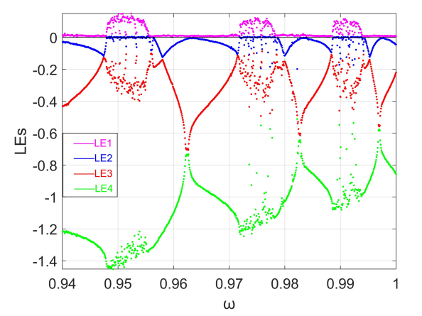
The Lyapunov exponents are significantly influenced by the system parameters \(p= 0.1,\ k=26\), and \(v=1\), with initial values \((2,2,2,2)\), where \(\omega\) is in the interval \((0.94,1]\). In Figure 9, the greatest Lyapunov exponent is positive throughout a spectrum of \(\omega\), confirming the persistence of chaos across varying orders. This chart illustrates the significant role that the fractional derivative plays in modulating system stability and complexity. The corresponding numerical values of the Lyapunov exponents for different values of the fractional order \(\omega\) are listed in Table 2. For \(\omega=0.95,0.953,0.955\), and \(0.99\), the fractional-order system (15) exhibits two positive Lyapunov exponents, indicating the emergence of hyperchaotic dynamics. Although the second positive exponent is relatively small, additional numerical checks were performed to verify its robustness. In particular, longer integration times and different step sizes were tested, and the second Lyapunov exponent consistently remained positive after discarding transient dynamics.
Figure 7 presents the phase portraits and time series for the representative case \(\omega=0.99\). Compared with the chaotic attractor shown in Figure 6, the hyperchaotic attractor appears more irregular and denser in phase space. This increased complexity is associated with the presence of two positive Lyapunov exponents, which leads to exponential divergence along multiple independent directions and results in more complex and unpredictable system behavior.
| \(\omega\) | LE1 | LE2 | LE3 | LE4 |
|---|---|---|---|---|
| 0.942 | 0.0094 | -0.0457 | -0.3751 | -1.2308 |
| 0.95 | 0.1160 | 0.0022 | -0.2546 | -1.4178 |
| 0.953 | 0.1125 | 0.0009 | -0.2908 | -1.373 |
| 0.955 | 0.0586 | 0.0010 | -0.2565 | -1.3091 |
| 0.96 | 0.0104 | -0.0486 | -0.3260 | -1.0958 |
| 0.97 | 0.0119 | -0.0621 | -0.2467 | -1.0695 |
| 0.98 | 0.0147 | -0.1101 | -0.1565 | -1.0256 |
| 0.99 | 0.0970 | 0.0017 | -0.2500 | -1.0416 |
| 0.999 | 0.0110 | -0.0223 | -0.2977 | -0.8120 |
| 1 | 0.0102 | -0.0499 | -0.2117 | -0.8617 |
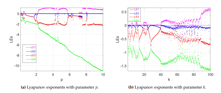
Furthermore, we examine the effect of parameters \(p\) and \(k\) individually, while keeping the remaining parameters fixed, with corresponding initial values \((2, 2, 2, 2)\) and fractional order \(\omega=0.96\). Figure 10 shows the variation of \(LE1,\ LE2,\ LE3\), and \(LE4\) with respect to parameters \(p\) and \(k\), respectively. Figures 10a and 10b reveal that chaos emerges in all values of \(p\) and \(k\) in the diagram, where \(LE1\) becomes positive or it stays near zero without crossing zero. This transition is indicative of a bifurcation in the system. \(LE2\) by negative remains near zero, while \(LE3\) and \(LE4\) stay negative, consistent with chaotic dynamics characterized by divergence in at least one direction. These Lyapunov exponents, which stay near zero, have been tested numerically to ensure the results. These findings underscore the importance of the parameters in influencing the stability and chaotic behavior of the fractional system (15).
The coexistence of attractors is confirmed by integrating the system from different initial conditions under identical parameters and observing distinct long-term behaviors.
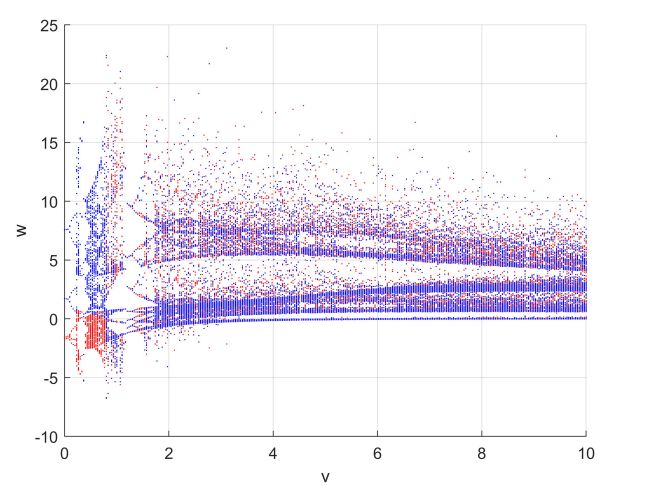
The parameter values \(p=9.5\) and \(k=10\) are considered in this section. We plot the bifurcation diagram of the \(w\)-peak in Figure 11 versus the control parameter \(v \in [0, 10]\), with \(\omega = 0.96\), and initial conditions \(X^+ = (2.3, 2.3, 0, 0)\) and \(X^- = (-2.3, -2.3, 0, 0)\). For higher values of \(v\), the system displays coexisting attractors, where one branch corresponds to stable periodic oscillations and the other to chaotic dynamics. This coexistence indicates strong sensitivity to initial conditions and highlights the multistability of the fractional-order system (15). Furthermore, as the parameter \(v\) diminishes, the coexistence attractor region approaches extinction. The stable periodic attractor undergoes a loss of stability via bifurcation, resulting in the system evolving into completely chaotic dynamics, particularly as \(v\) approaches zero. This transition demonstrates how the control parameter \(v\) determines the balance between stability and chaos.
Let parameter values \(p=9.5\), \(k=10\), and \(v=9.5\) be considered to show that the fractional-order system (15) displays a coexisting attractor. The equilibrium points of the system under these parameters are \((\pm \sqrt{10},\pm \sqrt{10},0,0)\), and the eigenvalues are \(\lambda_{1,2}=0.50508 \pm 4.4236i\) and \(\lambda_{3,4}=-10.005 \pm 0.73399i\). Using Theorem 3 the necessary condition for the occurrence of chaos is \[\begin{aligned} \omega \geq \frac{2}{\pi} \left( \tan^{-1} \left| \frac{4.4236}{0.50508} \right|\right)\approx 0.928. \end{aligned}\]
Consequently, the commensurate fractional order \(\omega\) must exceed \(0.928\) to preserve the instability of the eigenvalue.
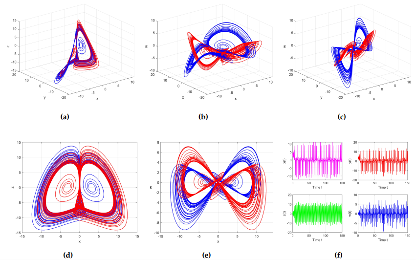
Figure 12 illustrates a family of self-excited attractors with stable as well as chaotic behavior under the initial condition \((2.3,2.3,0,0)\) and fractional-order \(\omega=0.96\), the Lyapunov exponents are \(LE1=0.0018,\ LE2=-0.2539, \ LE3=-9.0284\) and \(LE4=-12.2267\). Subfigures (12a–12e) show various phase portraits, where the trajectories display a clear coexistence of stable periodic orbits and chaotic motions, often forming multi-lobed or butterfly-like patterns. The symmetric arrangements emphasize the function of unstable equilibria to excite the attractors, and the order-chaos switching in the trajectories illustrates the multi-stability of the system. Finally, the corresponding time series of \(x(t), \ y(t), \ z(t)\), and \(w(t)\) in the subfigure 12f verify such coexistence, in which some signals collapse into regular oscillations. However, some oscillate chaotically, verifying the simultaneous existence of stability and chaos in the same dynamical regime. We also plot the phase portrait for \(v=0.6\) in Figure 13, which indicates the coexistence attractor region disappears and shows two scrolls. This leads to the system transitioning into almost entirely chaotic dynamics.
The coexistence reported here is demonstrated numerically by integrating the system from distinct initial conditions under identical parameters and observing different asymptotic behaviors. A full basin-of-attraction computation is beyond the scope of the present work.
The original integer-order system proposed by Huang et al. [45] exhibits chaotic dynamics for certain parameter settings; however, a Hopf bifurcation analysis was not reported for that model.
| Model | Parameters | Order | LEs | Behavior |
|---|---|---|---|---|
| Integer system [49] | \(\begin{aligned} \mathrm{p}&= 6\\ \mathrm{k} &= 11\\ \mathrm{v} &= 5\\ \end{aligned}\) | \(\omega=1\) | \(\begin{aligned} \mathrm{LE2}&= 0.5162\\ \mathrm{LE2} &= -0.0001\\ \mathrm{LE3} &= -4.9208\\ \mathrm{LE4} &= -6.5954 \end{aligned}\) | Chaos |
| Fractional system | \(\begin{aligned} \mathrm{p}&= 0.1\\ \mathrm{k} &= 26\\ \mathrm{v} &= 1\\ \end{aligned}\) | \(\omega=0.96\) | \(\begin{aligned} \mathrm{LE1} &= 0.010\\ \mathrm{LE2} &=-0.0486\\ \mathrm{LE3} &= -0.3260\\ \mathrm{LE4} &= -1.0958 \end{aligned}\) | Chaos |
| Fractional system | \(\begin{aligned} \mathrm{p}&= 0.1\\ \mathrm{k} &= 26\\ \mathrm{v} &= 1\\ \end{aligned}\) | \(\omega=0.99\) | \(\begin{aligned} \mathrm{LE1} &= 0.0970\\ \mathrm{LE2} &= 0.0017\\ \mathrm{LE3} &= -0.2500\\ \mathrm{LE4} &= -1.0416 \end{aligned}\) | Hyperchaos |
In the present work, a fractional-order extension is investigated under different parameter values and fractional orders. Although the parameter sets are not identical, the fractional-order formulation introduces fundamentally new dynamical features. In particular, the fractional order \(\omega\) serves as an effective bifurcation parameter, leading to stability changes and Hopf bifurcation phenomena that are absent in the integer-order case. Moreover, the fractional-order system exhibits chaos–hyperchaos transitions, richer attractor geometries, coexistence of attractors, and the emergence of hyperchaos characterized by two positive Lyapunov exponents; see Table 3. These results demonstrate that fractionalization significantly alters the system dynamics beyond a straightforward extension of the integer-order model.
In this paper, the fractional-order system (15) using the Caputo derivative was investigated. First, the stability and the occurrence of Hopf bifurcation at both equilibrium points were analyzed using the numerical predictor–corrector method, supported by the results in Figures 2–4. Then, bifurcation diagrams were presented for suitable parameter values satisfying the fractional-order conditions, highlighting different types of chaotic behavior such as self-excited attractors, coexisting attractors, and hyperchaotic dynamics at specific derivative orders.
Phase portraits for various fractional orders (Figures 6 and 7) and the largest Lyapunov exponents (Figures 8–10, Table 1) provide richer insight into the system’s dynamics. The occurrence of chaos and hyperchaos with varying fractional orders was confirmed through Table 2. Moreover, Figure 12 demonstrated the system’s multistability with coexisting attractors, while Figure 13 showed the transition from multistability to chaos as stability was lost. Overall, the results reveal that the fractional order and the control parameters significantly influence the dynamic behavior of the system.