
It has recently become evident that spectral methods [1– 5] form an important class of numerical techniques for solving significant problems in diverse scientific and engineering domains. Similar to other numerical techniques, these methods have several advantages; see, for example, [6– 8]. In particular, spectral methods usually produce highly accurate approximations with rapid convergence. There are three primary spectral approaches, each with its own advantages and applications. The selection of basis functions in the tau and collocation methods is less restrictive than in the Galerkin approach; see [9– 12]. References [13, 14] demonstrate that the Galerkin and Petrov–Galerkin approaches are effective for various problems. For further related research, we refer to [15– 22].
Schröder polynomials are valuable and useful in several domains, including control theory, signal processing, and cryptography, owing to their distinctive characteristics. These polynomials have also assumed increasingly important roles in approximation theory and numerical analysis. The authors in [9] employed SSPs in a numerical method for solving the nonlinear ordinary and fractional Newell–Whitehead–Segel equation. The authors in [23] used shifted Schröder polynomials within a numerical technique for solving the fractional Bagley–Torvik equation. In addition, several authors have examined these polynomials from a theoretical perspective, as reported in [24– 26].
Linear and nonlinear differential equations are well-established mathematical subjects with a systematic development that goes back to the beginning of calculus. Recent advances in mathematics have again shown that many phenomena in the applied sciences, described by differential equations, possess mathematical explanations because of the renewed and productive interaction among mathematics, science, and engineering. Numerous studies have addressed linear and nonlinear differential equations. The authors in [27] proposed an effective approach for solving linear and nonlinear singular initial and boundary value problems. The authors in [28] treated second-order delay differential equations using an innovative method. The authors in [29] solved nonlinear differential equations of the Lane–Emden type using a neural network methodology. For further related studies, see [30, 31].
The contributions of this paper can be summarized as follows:
We construct explicit spectral methods utilizing SSPs for linear and nonlinear SOTBVPs.
The proposed method transforms the considered problems into manageable systems of algebraic equations that can be solved using appropriate numerical techniques.
Extensive numerical experiments validate the accuracy and computational advantages of the proposed method.
The remaining sections of this work are organized as follows. The relevant characteristics of SSPs are presented in §2. In §3, we introduce a collocation spectral approach for the numerical solution of nonlinear SOTBVPs with homogeneous boundary conditions (HBCs). In §4, a Galerkin spectral method for the numerical treatment of linear SOTBVPs with HBCs is presented. §5 contains the illustrative examples and discussion of the numerical results, while §6 provides the concluding remarks.
The SSPs \(\psi_s(x)\) on the interval \([0,1]\) are defined by \(\psi_s(x)=\mathcal{S}_s(x-1)\), where \[\label{e2} \mathcal{S}_s(x)= \sum_{j=0}^s \frac{\binom{2j}{j}\binom{s+j}{s-j}}{j+1}\,x^j. \tag{1}\]
The following recurrence relation for \(\psi_s(x)\) is readily obtained by substituting \(x\) with \(x-1\) in the recurrence relation of \(\mathcal{S}_s(x)\) [24]: \[\label{e1} \left(x-\frac{1}{2}\right)\psi_{s}(x) =\frac{s-1}{2(2s+1)}\psi_{s-1}(x) +\frac{s+2}{2(2s+1)}\psi_{s+1}(x),\quad \psi_{0}(x)=1,\quad \psi_{1}(x)=x,\quad s\geq1. \tag{2}\]
The orthogonality condition of \(\psi_s(x)\) over the interval \([0,1]\) is \[\label{e5} \int_{0}^{1}\psi_s(x)\psi_n(x)\frac{1-x}{x}\,dx =\frac{1}{s(s+1)(2s+1)}\,\delta_{s,n}, \tag{3}\] where \(\delta_{s,n}\) is the Kronecker delta.
Corollary 1. [23] The first derivative of \(\psi_\ell(x)\) can be represented directly as \[\frac{d\psi_\ell(x)}{dx}= \sum_{s=0}^{\ell-1} \mathcal{F}_{s,\ell}\,\psi_s(x), \tag{4}\] where \[\label{e6f} \mathcal{F}_{s,\ell}=\frac{2s+1}{\ell(\ell+1)} \begin{cases} s^2+s+\ell^2+\ell, & \mbox{if }\,(\ell-s)\mbox{ is odd}, \\ (s-\ell)(s+\ell+1), & \mbox{otherwise}. \end{cases} \tag{5}\]
Corollary 2. [23] The second derivative of \(\psi_\ell(x)\) can be represented directly as follows: \[\frac{d^2\psi_\ell(x)}{dx^2}= \sum_{s=0}^{\ell-2} \sigma_{s,\ell}\,\psi_s(x), \tag{6}\] where \[\label{esig} \sigma_{s,\ell}=\frac{2s+1}{\ell(\ell+1)} \begin{cases} -(s-\ell-1)(s-\ell+1)(s+\ell)(s+\ell+2), & \mbox{if }\,(\ell-s)\mbox{ is odd}, \\ -(s-\ell)(s+\ell+1)\left(s^2+s+\ell^2+\ell-2\right), & \mbox{otherwise}. \end{cases} \tag{7}\]
Assume the following basis functions: \[\label{eah1} \rho_s(x)=(2s+3)\psi_{s+1}(x)-(s+1)(s+3)\psi_{s+2}(x)+s(s+2)\psi_s(x). \tag{8}\]
Remark 1. We note that the basis functions \(\rho_s(x)\), defined as linear combinations of the orthogonal polynomials \(\{\psi_s(x)\}\), are generally not orthogonal. However, the functions \(\rho_s(x)\) remain linearly independent and constitute a complete system in the approximation space, which is sufficient for the effective implementation of the Galerkin and collocation methods.
Using the derivative formulae for \(\psi_r(x)\) given in Corollaries 1 and 2, we derive the following two important results.
Corollary 3. The following formula holds: \[\frac{d\rho_s(x)}{dx} =(2s+3)\sum_{n=0}^{s}\mathcal{F}_{n,s+1}\psi_n(x) -(s+1)(s+3)\sum_{n=0}^{s+1}\mathcal{F}_{n,s+2}\psi_n(x) +s(s+2)\sum_{n=0}^{s-1}\mathcal{F}_{n,s}\psi_n(x), \tag{9}\] where \(\mathcal{F}_{n,s}\) is given in (5).
Proof. The proof follows directly from Eq. (8) and Corollary 1. ◻
Corollary 4. The following formula holds: \[\frac{d^2\rho_s(x)}{dx^2} =(2s+3)\sum_{j=0}^{s-1}\sigma_{j,s+1}\psi_j(x) -(s+1)(s+3)\sum_{j=0}^{s}\sigma_{j,s+2}\psi_j(x) +s(s+2)\sum_{j=0}^{s-2}\sigma_{j,s}\psi_j(x), \tag{10}\] where \(\sigma_{j,s}\) is given in (7).
Proof. The proof follows directly from Eq. (8) and Corollary 2. ◻
Consider the nonlinear SOTBVP \[\label{main1} \lambda''(x) = F(x,\lambda(x),\lambda'(x)), \tag{11}\] subject to the HBCs \[\lambda(0)=\lambda(1)=0. \tag{12}\]
Now, define the following function spaces: \[\begin{aligned} \Delta_{N}(0,1)&=\operatorname{span}\{\rho_s(x):0\le s\le N\},\\ \Lambda_{N}(0,1)&=\{\lambda(x)\in \Delta_{N}(0,1):\lambda(0)=\lambda(1)=0\}. \end{aligned}\]
Therefore, any \(\lambda(x)\in \Lambda_{N}(0,1)\) can be written as \[\label{eapp} \lambda(x)\approx \lambda_{N}(x)= \sum_{s=0}^N \hat{\lambda}_{s}\rho_s(x). \tag{13}\]
The residual \(\mathbf{R}_{1}(x)\) of Eq. (11), after using Corollaries 3 and 4, can be written as \[\begin{aligned} \label{ne.4} \mathbf{R}_{1}(x) &=\lambda_{N}''(x)-F(x,\lambda_{N}(x),\lambda_{N}'(x))\notag\\ &=\sum_{s=0}^N \hat{\lambda}_{s}\rho''_s(x) -F\left(x,\sum_{s=0}^N\hat{\lambda}_{s}\rho_s(x), \sum_{s=0}^N\hat{\lambda}_{s}\rho'_s(x)\right)\notag\\ &=\sum_{s=0}^N \hat{\lambda}_{s} \left((2s+3)\sum_{j=0}^{s-1}\sigma_{j,s+1}\psi_j(x) -(s+1)(s+3)\sum_{j=0}^{s}\sigma_{j,s+2}\psi_j(x) +s(s+2)\sum_{j=0}^{s-2}\sigma_{j,s}\psi_j(x)\right)\notag\\ &\quad -F\left(x,\sum_{s=0}^N \hat{\lambda}_{s}\rho_s(x), \sum_{s=0}^N \hat{\lambda}_{s}\left[ (2s+3)\sum_{n=0}^{s}\mathcal{F}_{n,s+1}\psi_n(x)\right.\right.\notag\\ &\quad\left.\left. -(s+1)(s+3)\sum_{n=0}^{s+1}\mathcal{F}_{n,s+2}\psi_n(x) +s(s+2)\sum_{n=0}^{s-1}\mathcal{F}_{n,s}\psi_n(x)\right]\right). \end{aligned} \tag{14}\]
The application of the collocation method leads to \[\begin{aligned} \label{collo} &\sum_{s=0}^N \hat{\lambda}_{s} \left((2s+3)\sum_{j=0}^{s-1}\sigma_{j,s+1}\psi_j(x_j) -(s+1)(s+3)\sum_{j=0}^{s}\sigma_{j,s+2}\psi_j(x_j) +s(s+2)\sum_{j=0}^{s-2}\sigma_{j,s}\psi_j(x_j)\right)\notag\\ &\quad -F\left(x_j,\sum_{s=0}^N \hat{\lambda}_{s}\rho_s(x_j), \sum_{s=0}^N \hat{\lambda}_{s}\left[ (2s+3)\sum_{n=0}^{s}\mathcal{F}_{n,s+1}\psi_n(x_j)\right.\right.\notag\\ &\quad\left.\left. -(s+1)(s+3)\sum_{n=0}^{s+1}\mathcal{F}_{n,s+2}\psi_n(x_j) +s(s+2)\sum_{n=0}^{s-1}\mathcal{F}_{n,s}\psi_n(x_j)\right]\right)=0, \quad j=1,2,\ldots,N+1. \end{aligned} \tag{15}\]
Ultimately, Eq. (15) represents a system of \((N+1)\) algebraic equations that can be solved using Newton’s iterative method.
Remark 2. The collocation points \(x_j\) are chosen as the roots of the shifted Schröder polynomial \(\psi_{N+1}(x)\) in the interval \((0,1)\).
Remark 3. It is worth mentioning that Newton’s method for solving the \((N+1)\) nonlinear system of equations is convergent under the following conditions:
A suitable initial guess, such as \(\hat{\lambda}_{s}=10^{-s}\), is chosen to ensure convergence.
The Jacobian matrix is nonsingular during the solution of the system in (15).
Consider the linear SOTBVP \[\label{main2} \lambda''(x)+f_1(x)\lambda'(x)+f_2(x)\lambda(x)=g(x), \quad x\in(0,1), \tag{16}\] subject to the HBCs \[\lambda(0)=\lambda(1)=0, \tag{17}\] where \(f_1(x)\), \(f_2(x)\), and \(g(x)\) are given continuous functions.
Using the approximation (13), we can write the residual of Eq. (16) as \[\label{ne.44} \mathbf{R}_{2}(x)=\lambda_{N}''(x)+f_1(x)\lambda_{N}'(x)+f_2(x)\lambda_{N}(x)-g(x). \tag{18}\]
The use of the Galerkin method leads to \[\label{galer} \int_{0}^{1}\mathbf{R}_{2}(x)\rho_s(x)\omega(x)\,dx=0,\quad s=0,1,\ldots,N. \tag{19}\]
The system resulting from Eq. (19) contains \((N+1)\) algebraic equations, which can be solved using the Gaussian elimination method.
Remark 4. The runtime of our method is significantly affected by solving the
linear system of size \((N+1)\) arising
from Eq. (19). The Gaussian elimination method is
implemented using NSolve in Mathematica 11, and the
computational cost per iteration is roughly \(O(N^3)\).
Remark 5. Based on the transformation \[v(x)=\lambda(x)-(1-x)\lambda(0)-x\lambda(1), \tag{20}\] we can transform Eqs. (11) and (16), subject to the following non-HBCs \[\lambda(0)=q_{1}, \quad \lambda(1)=q_{2}, \quad x\in(0,1), \tag{21}\] into problems with homogeneous boundary conditions.
Example 1. Consider the following equation [32]: \[2\lambda'' = (\lambda+x+1)^3,\quad 0<x<1, \tag{22}\] subject to \[\lambda(0)=0,\quad \lambda(1)=0, \tag{23}\] where the exact solution is \[\lambda(x)=\frac{2}{2-x}-x-1. \tag{24}\]
| \(N\) | 6 | 8 | 10 | 12 | 16 | 18 |
| Error | \(1.40062\times 10^-6\) | \(4.73652\times 10^-8\) | \(7.49971\times 10^-10\) | \(4.16188\times 10^-11\) | \(2.91711\times 10^-14\) | \(9.4369\times 10^-16\) |
| CPU time | 1.564 | 1.723 | 2.657 | 3.046 | 3.469 | 3.406 |
| Method | Sinc–Galerkin method in [32] | Present method |
|---|---|---|
| \(N\) | 130 | 18 |
| Error | \(9.992\times10^{-16}\) | \(9.4369\times10^{-16}\) |
| \(x\) | \(\mathrm{AEs}\) | CPU time | Relative \(\mathrm{AEs}\) | CPU time |
|---|---|---|---|---|
| 0.1 | \(1.73472\times10^{-16}\) | \(3.66219\times10^{-15}\) | ||
| 0.2 | \(2.498\times10^{-16}\) | \(2.81025\times10^{-15}\) | ||
| 0.3 | \(1.11022\times10^{-16}\) | \(8.98752\times10^{-16}\) | ||
| 0.4 | \(1.94289\times10^{-16}\) | \(1.29526\times10^{-15}\) | ||
| 0.5 | \(6.10623\times10^{-16}\) | 3.012 | \(3.66374\times10^{-15}\) | 3.138 |
| 0.6 | \(3.60822\times10^{-16}\) | \(2.1048\times10^{-15}\) | ||
| 0.7 | \(2.22045\times10^{-16}\) | \(1.37456\times10^{-15}\) | ||
| 0.8 | \(9.4369\times10^{-16}\) | \(7.07767\times10^{-15}\) | ||
| 0.9 | \(7.63278\times10^{-16}\) | \(9.32896\times10^{-15}\) |
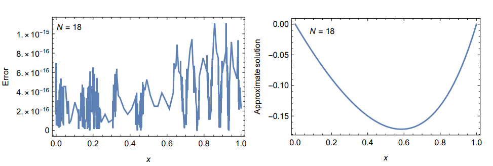
Table 1 presents the maximum absolute errors \(\mathrm{AEs}\). Table 2 compares the Sinc–Galerkin strategy from [32] with the present method for \(N=18\). Table 3 reports the \(\mathrm{AEs}\) and relative \(\mathrm{AEs}\) for \(N=18\) at selected points. These results show that our technique produces an extremely accurate approximation of the exact solution. Figure 1 shows the \(\mathrm{AEs}\) on the left and the approximate solution (AS) on the right for \(N=18\). This figure reveals that the suggested strategy consistently reduces errors across the domain and shows a high level of agreement between the approximate and exact solutions.
Example 2. Consider the following equation: \[\lambda''(x)-\lambda'(x)^3+\lambda(x)=-64x^9+x^4+12x^2, \tag{25}\] subject to \[\lambda(0)=0,\quad \lambda(1)=1, \tag{26}\] where the exact solution of this problem is \[\lambda(x)=x^4. \tag{27}\]
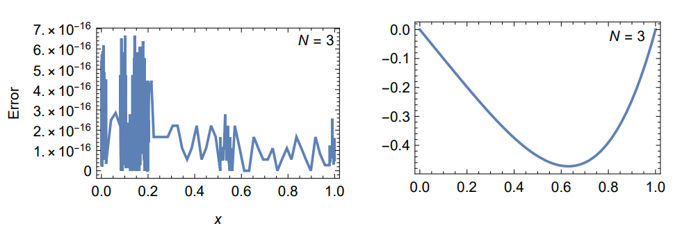
Table 4 displays the \(\mathrm{AEs}\) and relative \(\mathrm{AEs}\) for \(N=3\). Figure 2 shows the \(\mathrm{AEs}\) on the left and the AS on the right for \(N=3\). These results demonstrate that the proposed approach consistently reduces errors across the domain and that the approximate solution is in good agreement with the exact solution.
| \(x\) | \(\mathrm{AEs}\) | CPU time | Relative \(\mathrm{AEs}\) | CPU time |
| 0.1 | \(1.38778\times10^-17\) | \(1.38917\times10^-16\) | ||
| 0.2 | \(2.77556\times10^-17\) | \(1.39897\times10^-16\) | ||
| 0.3 | \(5.55112\times10^-17\) | \(1.90172\times10^-16\) | ||
| 0.4 | \(0\) | \(0\) | ||
| 0.5 | \(5.55112\times10^-17\) | 1.201 | \(1.26883\times10^-16\) | 1.312 |
| 0.6 | \(1.11022\times10^-16\) | \(2.36017\times10^-16\) | ||
| 0.7 | \(1.11022\times10^-16\) | \(2.41405\times10^-16\) | ||
| 0.8 | \(0\) | \(0\) | ||
| 0.9 | \(2.77556\times10^-17\) | \(1.13799\times10^-16\) |
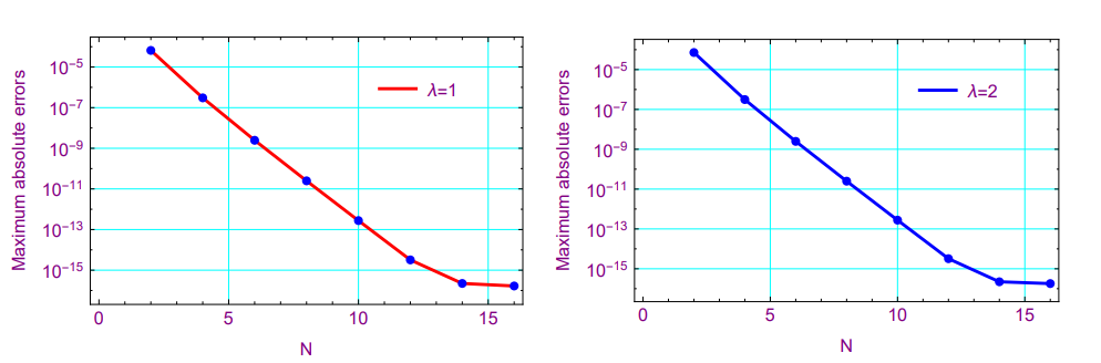
Example 3. Consider the following Bratu equation [33]: \[\label{eq:bratu} \lambda''(x)+\lambda e^{\lambda(x)}=0, \tag{28}\] subject to \[\lambda(0)=0,\quad \lambda(1)=0, \tag{29}\] with the analytical solution \[\lambda(x)=-\log\left(\frac{\cosh\left(\frac{1}{4}\theta(2x-1)\right)}{\cosh\left(\frac{\theta}{4}\right)}\right), \tag{30}\] where \(\theta\) is the solution of the nonlinear equation \[\theta=\sqrt{2\lambda}\cosh\theta.\] The described technique is used to numerically solve Eq. (28) for the two cases corresponding to \(\lambda=1\) and \(\lambda=2\), resulting in \(\theta=1.51716\) and \(\theta=2.35755\), respectively.
The maximum \(\mathrm{AEs}\) are presented in Table 5. Figure 3 illustrates the maximum \(\mathrm{AEs}\) for various values of \(N\) and \(\lambda\). These results show that the suggested strategy reduces errors consistently throughout the domain and demonstrates good agreement between the approximate and exact solutions.
| \(\lambda=1\) | \(\lambda=2\) | ||
| Method in [33] at \(N=18\) | Present method at \(N=16\) | Method in [33] at \(N=18\) | Present method at \(N=16\) |
| \(2.983\times10^-16\) | \(1.66533\times10^-16\) | \(4.024\times10^-16\) | \(1.80411\times10^-16\) |
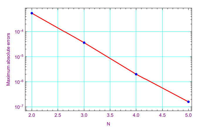
Example 4. Consider the following equation: \[\label{eq:example4} \lambda''(x)+\lambda'(x)+\lambda(x)=3e^x, \tag{31}\] subject to \[\lambda(0)=1,\quad \lambda(1)=e, \tag{32}\] with the analytical solution \[\lambda(x)=e^x. \tag{33}\]
The \(\mathrm{AEs}\) and relative \(\mathrm{AEs}\) at \(N=5\) are shown in Table 6. Moreover, the maximum \(\mathrm{AEs}\) for different values of \(N\) are shown in Figure 4. These results verify that the suggested approach reduces errors consistently throughout the domain and shows good agreement between the approximate and exact solutions.
| \(x\) | \(\mathrm{AEs}\) | CPU time | Relative \(\mathrm{AEs}\) | CPU time |
|---|---|---|---|---|
| 0.1 | \(1.22113\times10^{-7}\) | \(1.83195\times10^{-6}\) | ||
| 0.2 | \(1.51506\times10^{-7}\) | \(1.23928\times10^{-6}\) | ||
| 0.3 | \(1.59315\times10^{-7}\) | \(9.61898\times10^{-7}\) | ||
| 0.4 | \(1.51545\times10^{-7}\) | \(7.75214\times10^{-7}\) | ||
| 0.5 | \(1.30842\times10^{-7}\) | 2.152 | \(6.21817\times10^{-7}\) | 2.283 |
| 0.6 | \(1.05088\times10^{-7}\) | \(5.03173\times10^{-7}\) | ||
| 0.7 | \(7.93369\times10^{-8}\) | \(4.19673\times10^{-7}\) | ||
| 0.8 | \(5.26598\times10^{-8}\) | \(3.53221\times10^{-7}\) | ||
| 0.9 | \(2.48884\times10^{-8}\) | \(2.86566\times10^{-7}\) |
Example 5. Consider the following equation: \[\label{eq:example5} \lambda''(x)+x\lambda'(x)-\lambda(x)=4x^3(x^2+5), \tag{34}\] subject to \[\lambda(0)=0,\quad \lambda(1)=1, \tag{35}\] with the analytical solution \[\lambda(x)=x^5. \tag{36}\]
| \(x\) | \(\mathrm{AEs}\) | Relative \(\mathrm{AEs}\) |
|---|---|---|
| 0.1 | \(5.55112\times10^{-17}\) | \(5.55167\times10^{-16}\) |
| 0.2 | \(8.32667\times10^{-17}\) | \(4.17001\times10^{-16}\) |
| 0.3 | \(5.55112\times10^{-17}\) | \(1.86548\times10^{-16}\) |
| 0.4 | \(5.55112\times10^{-17}\) | \(1.86548\times10^{-16}\) |
| 0.5 | \(0\) | \(0\) |
| 0.6 | \(5.55112\times10^{-17}\) | \(4.25177\times10^{-16}\) |
| 0.7 | \(2.22045\times10^{-16}\) | \(2.08716\times10^{-16}\) |
| 0.8 | \(1.11022\times10^{-16}\) | \(2.35057\times10^{-16}\) |
| 0.9 | \(5.55112\times10^{-17}\) | \(1.79352\times10^{-16}\) |
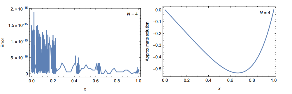
The \(\mathrm{AEs}\) and relative \(\mathrm{AEs}\) at \(N=4\) are presented in Table 7. Figure 5 displays the \(\mathrm{AEs}\) on the left and the AS on the right for \(N=4\). These findings confirm that the recommended method consistently reduces errors across the domain and demonstrates a high degree of agreement between the approximate and exact solutions.
This paper presents and analyzes an accurate solver based on Galerkin and collocation techniques for particular linear and nonlinear SOTBVPs. Certain theoretical results related to SSPs play an important role in applying the proposed numerical methods to solve linear and nonlinear SOTBVPs. A variety of numerical experiments and comparisons have been presented to demonstrate the validity and effectiveness of the proposed approach. Moreover, the method can be extended to more general models arising in various areas of physics, mathematics, and engineering.