
Nonlinear systems of equations (SNE) are fundamental in a wide range of fields, from scientific research to various engineering applications. These systems are distinguished by their complexity and by the intricate relationships among variables, which often necessitate the use of advanced solution techniques. Consequently, researchers are motivated to develop effective iterative methods to address the challenges presented by these nonlinear equations [2– 6]. The primary aim of these methods is to achieve accurate solutions while minimizing the computational resources required for their determination.
A nonlinear system of equations is typically represented in the following mathematical form: \[\label{a1} \mathfrak{F}(s)=0. \tag{1}\] In this expression, \(\mathfrak{F}:\mathbb{R}^n\to\mathbb{R}^n\) denotes a nonlinear mapping that connects inputs from the \(n\)-dimensional real space to their corresponding output values. In this paper, we refer to \(\mathbb{R}^n\) as the \(n\)-dimensional real space, and we use the notation \(\|\cdot\|\) to denote the Euclidean norm, which serves as a standard measure of distance in this context. By investigating these systems and the methods for solving them, we aim to contribute meaningful insights to the field.
To solve problem (1), various iterative techniques can be employed. These techniques include double-direction methods [7– 10], double-step-length methods [11– 16], Newton’s method (NM) [2], and quasi-Newton methods (QNM) [6, 17]. Among these techniques, NM stands out due to its favorable characteristics, such as ease of implementation and rapid convergence. However, the Jacobian matrix (JM) must be computed and stored during each iteration. These techniques use the recursive formula to generate a sequence of points: \[\label{h3} s_{k+1}=s_k+\alpha_k q_k,\qquad k=0,1,\ldots, \tag{2}\] where \(\alpha_k\) is the step size, \(q_k\) is the search direction, and the current and next iterates are \(s_k\) and \(s_{k+1}\), respectively. The NM search direction \(q_k\) is determined by \[\label{ND} q_k=-(\mathfrak{F}^{\prime}(s_k))^{-1}\mathfrak{F}(s_k).\] Here, \(\mathfrak{F}^{\prime}(s_k)\) is the JM of \(\mathfrak{F}\) at \(s_k\). However, one limitation of Newton’s method is that it requires the derivative, namely the JM, to be computed at each iteration, which may not always be available or may not be precisely determined. In such cases, NM cannot be applied directly.
The global optimization problem can be derived from (1) [1]. Let \(\mathfrak{h}\) be a merit function given by \[\label{a7} \mathfrak{h}(s)=\frac{1}{2}\|\mathfrak{F}(s)\|^{2}. \tag{3}\] Consequently, problem (1) can be equivalently expressed as the following global optimization problem: \[\label{global} \min \mathfrak{h}(s),\qquad s\in\mathbb{R}^n,\qquad \mathfrak{h}:\mathbb{R}^n\to\mathbb{R}. \tag{4}\]
In order to achieve global convergence, it is essential to employ a step length in iterative methods. This is because the use of a step length reduces the function value, thereby helping to ensure global convergence. For instance, NM is locally convergent. However, NM becomes globally convergent when equipped with a step length. In addition, the step length can be computed using any suitable line-search technique. The exact line search is appropriate for use in practice [18] and satisfies \[\label{ab1} \mathfrak{h}(s_k+\alpha_k q_k) = \min_{\alpha>0}\mathfrak{h}(s_k+\alpha q_k). \tag{5}\]
In practical applications, determining the precise value of the step length is often challenging. Consequently, inexact line-search methods are the predominant approach used in practice [16, 19, 20]. In this regard, the authors in [21] introduced a specific line-search rule that effectively identifies an appropriate step length: \[\label{bb1} \mathfrak{h}(s_k+\alpha_k q_k)-\mathfrak{h}(s_k) \leq \sigma\alpha_k\nabla \mathfrak{h}(s_k)^Tq_k, \qquad \sigma\in(0,1). \tag{6}\]
The technique outlined in (6) indicates that the JM must be calculated at every iteration. This requirement has the potential to substantially increase computational demands, especially in the context of large-scale problems or when dealing with complex matrix calculations. To address these concerns, Yuan\(^*\) and Lu [17] proposed a new backtracking inexact technique for determining the step length \(\alpha_k\) as follows: \[\label{bb2} \|\mathfrak{F}(s_k+\alpha_k q_k)\|^2 \leq \|\mathfrak{F}(s_k)\|^2+\phi\alpha_k^2\mathfrak{F}(s_k)^Tq_k,\] where \(\phi\in(0,1)\). Another inexact line search was introduced in [1], and the step length can be calculated as follows.
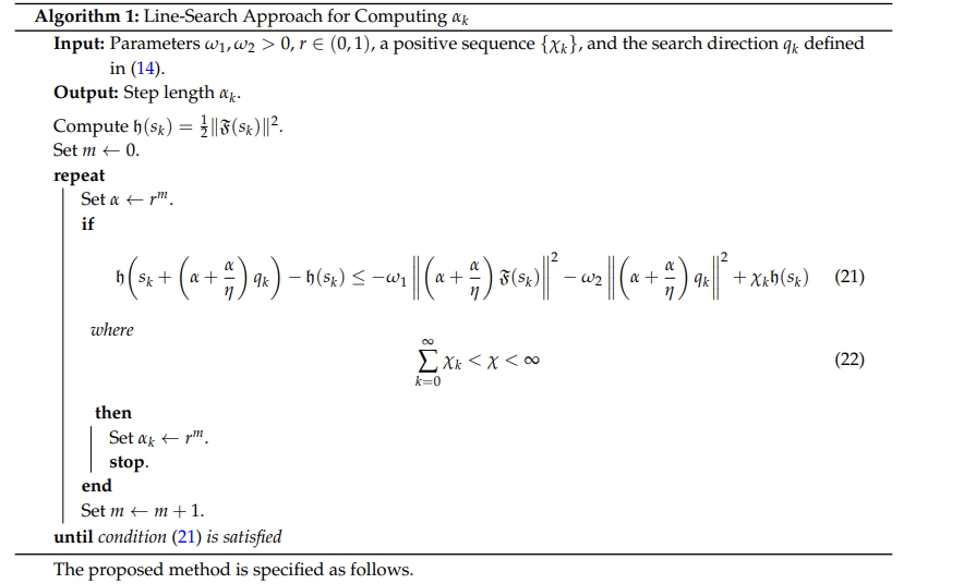
Let \(r\in(0,1)\), \(\omega_1,\omega_2>0\), and let \(\{\chi_k\}\) be a given positive sequence such that \[\label{ab29} \sum_{k=0}^{\infty}\chi_k<\chi<\infty.\] Then the step length is chosen to satisfy \[\label{a30} \mathfrak{h}(s_k+\alpha_k q_k)-\mathfrak{h}(s_k) \leq -\omega_1\|\alpha_k\mathfrak{F}(s_k)\|^2 -\omega_2\|\alpha_k q_k\|^2 +\chi_k\mathfrak{h}(s_k).\]
Despite the favorable properties of NM, it requires the computation of the Jacobian or its approximation at each iteration. This requirement makes it less suitable for large-scale problems, as it necessitates extensive matrix storage, which can be costly in numerical experiments. To address these concerns, matrix-free approaches have been proposed. The double-direction method (DDM) is one such successful matrix-free approach [10], which generates the iterates using the following formula: \[\label{dd} s_{k+1}=s_k+\alpha_k q_k+\alpha_k^2 b_k, \tag{7}\] where \(q_k\) and \(b_k\) are the respective search directions. The essential idea underlying the DDM is that it incorporates two adjustments in the system represented by (7). If one correction fails, the other serves as a backup to correct the system.
In their work, Petrovi\(\acute{c}\) and Stanimirovi\(\acute{c}\) [10] made significant contributions to the field of unconstrained optimization by proposing a DDM. This innovative approach utilizes an acceleration parameter \(\delta_k>0\) to construct an approximation of the Hessian matrix, which is expressed as \[\nabla^2\mathfrak{h}(s_k)\approx \delta_k I,\] where \(I\) denotes the identity matrix and the acceleration parameter is given by \[\delta_{k+1}^{ADD} = 2 \frac{ \mathfrak{h}(s_{k+1})-\mathfrak{h}(s_k) -\alpha_k\nabla\mathfrak{h}(s_k)^T \bigl(\alpha_kq_k-\delta_k^{-1}\nabla\mathfrak{h}(s_k)\bigr) }{ \bigl(\alpha_kq_k-\delta_k^{-1}\nabla\mathfrak{h}(s_k)\bigr)^T \bigl(\alpha_kq_k-\delta_k^{-1}\nabla\mathfrak{h}(s_k)\bigr) }.\]
To enhance the efficiency of the DDM presented in [10], Petrovi\(\acute{c}\) further refined it in [16] by introducing a double-step-length scheme (DSM). This was done by replacing \(\alpha_k^2\) in (7) with \(\beta_k\), which is defined mathematically as \[\label{dsl} s_{k+1}=s_k+\alpha_k q_k+\beta_k b_k. \tag{8}\] In the above equation, \(\alpha_k\) and \(\beta_k\) represent two independently chosen step sizes, allowing for a more flexible and adaptive approach to convergence. In addition, the proposed acceleration parameter is given by \[\delta_{k+1}^{ADSS} = 2 \frac{ \mathfrak{h}(s_{k+1})-\mathfrak{h}(s_k) + (\alpha_k\delta_k^{-1}+\beta_k)\|\nabla\mathfrak{h}(s_k)\|^2 }{ (\alpha_k\delta_k^{-1}+\beta_k)^2\|\nabla\mathfrak{h}(s_k)\|^2 }.\]
The numerical results in [16] illustrate that this refined method demonstrates superior performance compared with the original DDM, achieving a reduction in the number of iterations required as well as a decrease in processor time.
The existing literature on derivative-free DDM for solving SNE is notably limited. This lack of comprehensive research inspired Halilu and Waziri [8] to develop a derivative-free method that employs a DDM for addressing (1), as described in Eq. (7). The approach proposed an acceleration parameter \(\delta_k>0\) to create an approximation of the Jacobian matrix, expressed as \[\label{AC} \mathfrak{F}^{\prime}(s_k)\approx \delta_k I. \tag{9}\] The acceleration parameter is given by \[\delta_{k+1}^{IDFDD} = \frac{v_k^Tv_k} {(\alpha_k+\alpha_k^2\delta_k)v_k^Tq_k},\] where \[v_k=\mathfrak{F}(s_{k+1})-\mathfrak{F}(s_k).\] Subsequently, in [22], a modified version of the algorithm in [8] was developed. They established that the proposed method exhibits global convergence, contingent on the condition that the JM is both positive definite and bounded. This finding is significant, as it lays the groundwork for reliable solutions to nonlinear equations without requiring derivatives.
Building upon this framework, Abdullahi et al. [7] made substantial improvements to the performance of the DDM. They modified the initial methodology from [8] by integrating a conjugate-gradient approach for symmetric nonlinear equations. Their enhancement not only retained the derivative-free nature of the method but also facilitated global convergence, achieved through the innovative line-search strategy proposed by Li and Fukushima [1]. This advancement marks notable progress in the efficiency and applicability of DDM for solving SNE.
In another contribution, Halilu and Waziri [9] further refined the DDM discussed in (7) for solving SNE. Their latest method demonstrates global convergence under some mild assumptions, which broadens its applicability. The research includes extensive numerical experiments that validate the efficiency and effectiveness of their proposed method, showcasing promising results that contribute to the ongoing development of robust techniques for solving SNE in a derivative-free manner.
In their insightful study presented in [13], the authors effectively built upon the foundational concepts in Eq. (8) by introducing the DSM. Here, the acceleration parameter is given by \[\label{a16} \delta_{k+1} = \frac{v_k^Tv_k} {(\alpha_k+\beta_k)v_k^Tq_k}.\] This innovative method aims to enhance the efficacy of the DDM described in [8]. The results from their research are particularly encouraging, as they indicate that the DSM leads to significantly faster convergence than the previous method. These findings not only highlight the potential of their approach to optimize numerical algorithms but also pave the way for further advancements in this area of study.
It has been observed that the DSM for unconstrained optimization problems [16] and the DSM for SNE [13] use a line-search approach to determine the values of the two step lengths. Motivated by these concepts, our objective is to develop an improved DSM for solving SNE, where the two step lengths can be computed using a different line-search approach in order to improve both the efficiency and accuracy of the DDM in finding solutions to Problem (1).
The structure of the paper is as follows. The derivation of the suggested approach is explained in the next section. A convergence analysis of the suggested algorithm is given in §3. A number of numerical tests and motion-control applications of the suggested method are presented in §4. The article is concluded in §5.
In this section, we present a derivative-free approach for solving SNE using an acceleration parameter. We begin by recalling the derivative-free spectral method (DSM) introduced in [13], where the iterative sequence \(\{s_k\}\) is generated by \[\label{schm} s_{k+1}=s_k+\alpha_k q_k+\beta_k q_k, \tag{10}\] and the search direction is defined as \[\label{ash18-old} q_k=-\delta_k^{-1}\mathfrak{F}(s_k). \tag{11}\]
Subsequently, in [15], a double-step-length strategy was proposed by defining two search directions in the double-step-length iteration (7) as \[\label{ash18a} q_k=-\eta\delta_k^{-1}\mathfrak{F}(s_k), \tag{12}\] and \[\label{ash18b} b_k=-\mathfrak{F}(s_k), \tag{13}\] where \(\eta\in(1,2)\) is a correction parameter obtained by hybridizing the double-step-length iteration with the Picard–Mann process [23].
Although the DSM proposed in [13] is fully derivative-free and computationally efficient, its reliance on a single acceleration parameter \(\delta_k\) may limit its effectiveness. In particular, when \(\delta_k=1\), the method reduces to a steepest-descent-type iteration, which may result in slow convergence. The double-step-length strategy introduced in [15] incorporates a correction parameter \(\eta\) through hybridization with the Picard–Mann process, leading to improved numerical performance. However, the method employs two distinct search directions, one of which coincides with the classical steepest-descent direction, which is known to converge slowly in certain situations. This may affect the consistency of the update scheme and prevent the method from fully exploiting the acceleration effect of the correction parameter across all directions.
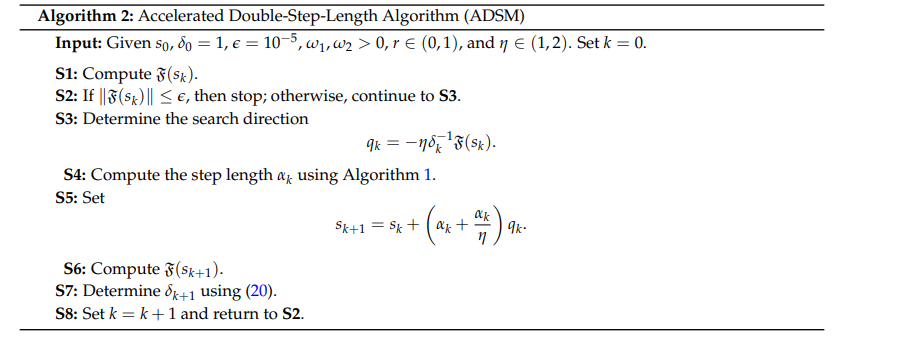
Motivated by these observations, we propose a simplified accelerated derivative-free scheme by reducing the two directions to a single search direction: \[\label{ash18} q_k=-\eta\delta_k^{-1}\mathfrak{F}(s_k). \tag{14}\] This choice integrates both the acceleration and correction parameters into a single direction. This reduction addresses the identified gaps by:
maintaining uniform acceleration and correction through the parameter \(\eta\) in all iterations;
avoiding the slow convergence associated with the steepest-descent direction;
reducing computational cost by eliminating the need to compute two separate directions.
To further reduce computational effort, we assume a relationship between the step lengths \(\alpha_k\) and \(\beta_k\) as \[\label{betak} \beta_k=\frac{\alpha_k}{\eta}. \tag{15}\]
Remark 1. The proposed search direction incorporates both acceleration and correction parameters. Moreover, since \(\eta\in(1,2)\), the direction \(q_k\) never reduces to the classical steepest-descent direction, thereby avoiding its potential slow convergence behavior.
Next, we update the acceleration parameter \(\delta_{k+1}\) using the Taylor series expansion below: \[\label{a23a} \mathfrak{F}(s_{k+1}) \approx \mathfrak{F}(s_k)+\mathfrak{F}^{\prime}(\xi)(s_{k+1}-s_k), \tag{16}\] where \(\xi\in[s_k,s_{k+1}]\) can be expressed as \[\xi=s_k+\varrho(s_{k+1}-s_k),\qquad 0\leq\varrho\leq1.\] By selecting \(\varrho=1\), we have \[\label{a23ab} \mathfrak{F}(s_{k+1}) \approx \mathfrak{F}(s_k)+\mathfrak{F}^{\prime}(s_{k+1})(s_{k+1}-s_k). \tag{17}\]
To make the computations more efficient, we use a diagonal matrix to approximate the JM. This approximation eliminates the need for complex computations and storage associated with the full JM, thereby simplifying the overall procedure. Consequently, we use the approximation \[\label{a25a} \mathfrak{F}^{\prime}(s_{k+1})\approx \delta_{k+1}I. \tag{18}\]
Thus, based on (17) and (18), it is straightforward to verify the following secant equation: \[\label{a23ac} v_k\approx \delta_{k+1}u_k, \tag{19}\] where \[u_k=s_{k+1}-s_k = \left(\alpha_k+\frac{\alpha_k}{\eta}\right)q_k\] and \[v_k=\mathfrak{F}(s_{k+1})-\mathfrak{F}(s_k).\] By multiplying both sides of (19) by the transpose of \(v_k\), we obtain the following update for the acceleration parameter: \[\label{AP} \delta_{k+1} \approx \frac{v_k^Tv_k} {\left(\alpha_k+\frac{\alpha_k}{\eta}\right)v_k^Tq_k}. \tag{20}\]
Remark 2. The proposed acceleration parameter \(\delta_{k+1}\) is positive. Indeed, the numerator \(v_k^Tv_k>0\), provided that the solution has not yet been reached. Moreover, from Lemma 3 in the convergence analysis section, the denominator satisfies \[\left(\alpha_k+\frac{\alpha_k}{\eta}\right)v_k^Tq_k>0,\] ensuring that \(\delta_{k+1}\) is well defined and strictly positive at each iteration.
The procedure for computing the step length is summarized in Algorithm 1.
In this section, we present the global convergence analysis of the proposed Algorithm 2, namely the Accelerated Double-Step-Length Method (ADSM). We begin by defining the level set \[\label{a46} \Omega=\{s\mid \|\mathfrak{F}(s)\|\leq \|\mathfrak{F}(s_0)\|\}. \tag{23}\]
Assumption 1. The following assumptions are imposed:
There exists \(s^*\in\mathbb{R}^n\) such that \(\mathfrak{F}(s^*)=0\).
The function \(\mathfrak{F}(s)\) is continuously differentiable in some neighborhood, say \(Q\), of \(s^*\) containing \(\Omega\).
The Jacobian matrix \(\mathfrak{F}'(s)\) is positive definite and bounded on \(Q\); that is, there exist constants \(H_1>H_2>0\) such that \[\label{a47} \|\mathfrak{F}'(s)\|\leq H_1,\qquad \forall s\in Q, \tag{24}\] and \[\label{a48} H_2\|q\|^{2}\leq q^{T}\mathfrak{F}'(s)q,\qquad \forall s\in Q,\quad q\in\mathbb{R}^n. \tag{25}\]
Remark 3. Assumption 1 implies that there exist constants \(H_1>H_2>0\) such that \[\label{a49} H_2\|q\|\leq \|\mathfrak{F}'(s)q\|\leq H_1\|q\|,\qquad \forall s\in Q,\quad q\in\mathbb{R}^n, \tag{26}\] and \[\label{a50} H_2\|s-v\|\leq \|\mathfrak{F}(s)-\mathfrak{F}(v)\|\leq H_1\|s-v\|,\qquad \forall s,v\in Q. \tag{27}\]
Since \(\eta^{-1}\delta_k I\) approximates \(\mathfrak{F}'(s_k)\) along \(s_k\), the following assumption can be made.
Assumption 2. The scaled identity matrix \(\eta^{-1}\delta_k I\) provides a local approximation of the Jacobian matrix \(\mathfrak{F}'(s_k)\) along the search direction \(q_k\). That is, we assume \[\label{a52} \|(\mathfrak{F}'(s_k)-\eta^{-1}\delta_k I)q_k\| \leq \epsilon\|\mathfrak{F}(s_k)\|, \tag{28}\] where \(\epsilon\in(0,1)\) is a small quantity.
Lemma 1. Let \(\{s_k\}\) be generated by the ADSM algorithm, and suppose that Assumption 2 holds. Then \(q_k\) is a sufficient descent direction for \(\mathfrak{h}(s_k)\) at \(s_k\); that is, \[\label{a27} \nabla\mathfrak{h}(s_k)^Tq_k\leq -c\|\mathfrak{F}(s_k)\|^{2},\qquad c>0. \tag{29}\]
Proof. From (3), (14), and (28), we have \[\begin{aligned} \label{a28} \nabla\mathfrak{h}(s_k)^Tq_k &= \mathfrak{F}(s_k)^T\mathfrak{F}'(s_k)q_k \notag\\ &= \mathfrak{F}(s_k)^T \left[ (\mathfrak{F}'(s_k)-\eta^{-1}\delta_k I)q_k-\mathfrak{F}(s_k) \right]\notag\\ &= \mathfrak{F}(s_k)^T(\mathfrak{F}'(s_k)-\eta^{-1}\delta_k I)q_k -\|\mathfrak{F}(s_k)\|^{2}. \end{aligned} \tag{30}\] Applying the Cauchy–Schwarz inequality, we obtain \[\begin{aligned} \label{a29} \nabla\mathfrak{h}(s_k)^Tq_k &\leq \|\mathfrak{F}(s_k)\| \|(\mathfrak{F}'(s_k)-\eta^{-1}\delta_k I)q_k\| -\|\mathfrak{F}(s_k)\|^{2} \notag\\ &\leq -(1-\epsilon)\|\mathfrak{F}(s_k)\|^{2}. \end{aligned} \tag{31}\] Since \(\epsilon\in(0,1)\), taking \(c=1-\epsilon\) proves the lemma.
From Lemma 1, we conclude that the norm function \(\mathfrak{h}(s_k)\) decreases along \(q_k\). Hence, \[\|\mathfrak{F}(s_{k+1})\|\leq \|\mathfrak{F}(s_k)\|.\] ◻
Lemma 2. Let \(\{s_k\}\) be generated by the ADSM algorithm, and suppose that Assumption 2 holds. Then \[\{s_k\}\subset \Omega.\]
Proof. From Lemma 1, we have \[\|\mathfrak{F}(s_{k+1})\|\leq \|\mathfrak{F}(s_k)\|.\] Furthermore, for all \(k\), \[\|\mathfrak{F}(s_{k+1})\| \leq \|\mathfrak{F}(s_k)\| \leq \|\mathfrak{F}(s_{k-1})\| \leq \cdots \leq \|\mathfrak{F}(s_0)\|.\] This implies that \(\{s_k\}\subset \Omega\). ◻
Lemma 3. Let \(\{s_k\}\) be generated by the ADSM algorithm, and suppose that Assumption 2 holds. Then there exists a constant \(H_2>0\) such that, for all \(k\), \[\label{a56} v_k^Tu_k\geq H_2\|u_k\|^{2}, \tag{32}\] where \[u_k=(\alpha_k+\beta_k)q_k.\]
Proof. By the mean-value theorem and (25), we obtain \[v_k^Tu_k = u_k^T\big(\mathfrak{F}(s_{k+1})-\mathfrak{F}(s_k)\big) = u_k^{T}\mathfrak{F}'(\xi)u_k \geq H_2\|u_k\|^{2},\] where \[\xi=s_k+\kappa(s_{k+1}-s_k),\qquad \kappa\in(0,1).\] Therefore, the result follows.
From Lemma 3 and (27), the following inequalities hold: \[\label{a33} \frac{v_k^Tu_k}{\|u_k\|^2}\geq H_2, \qquad \frac{v_k^Tv_k}{\left(\alpha_k+\frac{\alpha_k}{\eta}\right)v_k^Tq_k} \leq \frac{H_1^{2}}{H_2}. \tag{33}\] From (33), we conclude that the acceleration parameter in (20) is bounded. ◻
Lemma 4. Let \(\{s_k\}\) be generated by the ADSM algorithm, and suppose that Assumption 2 holds. Then \[\label{a58} \lim_{k\rightarrow\infty} \left\| \left(\alpha_k+\frac{\alpha_k}{\eta}\right)q_k \right\|=0, \tag{34}\] and \[\label{a59} \lim_{k\rightarrow\infty} \left\| \left(\alpha_k+\frac{\alpha_k}{\eta}\right)\mathfrak{F}(s_k) \right\|=0. \tag{35}\]
Proof. From (21), for all \(k>0\), we have \[\begin{aligned} \label{a60} \omega_2 \left\| \left(\alpha_k+\frac{\alpha_k}{\eta}\right)q_k \right\|^{2} &\leq \omega_1 \left\| \left(\alpha_k+\frac{\alpha_k}{\eta}\right)\mathfrak{F}(s_k) \right\|^{2} + \omega_2 \left\| \left(\alpha_k+\frac{\alpha_k}{\eta}\right)q_k \right\|^{2} \notag\\ &\leq \|\mathfrak{F}(s_k)\|^{2} – \|\mathfrak{F}(s_{k+1})\|^{2} + \chi_k\|\mathfrak{F}(s_k)\|^{2}. \end{aligned} \tag{36}\] By summing the above inequality, we obtain \[\begin{aligned} \label{a61} \omega_2 \sum_{i=0}^{k} \left\| \left(\alpha_i+\frac{\alpha_i}{\eta}\right)q_i \right\|^{2} &\leq \sum_{i=0}^{k} \left( \|\mathfrak{F}(s_i)\|^{2} – \|\mathfrak{F}(s_{i+1})\|^{2} \right) + \sum_{i=0}^{k} \chi_i\|\mathfrak{F}(s_i)\|^{2} \notag\\ &= \|\mathfrak{F}(s_0)\|^{2} – \|\mathfrak{F}(s_{k+1})\|^{2} + \sum_{i=0}^{k} \chi_i\|\mathfrak{F}(s_i)\|^{2} \notag\\ &\leq \|\mathfrak{F}(s_0)\|^{2} + \|\mathfrak{F}(s_0)\|^{2} \sum_{i=0}^{k}\chi_i \notag\\ &\leq \|\mathfrak{F}(s_0)\|^{2} + \|\mathfrak{F}(s_0)\|^{2} \sum_{i=0}^{\infty}\chi_i. \end{aligned} \tag{37}\] Based on the level set and the fact that the sequence \(\{\chi_k\}\) satisfies the criterion in (22), it follows that the series \[\sum_{i=0}^{\infty} \left\| \left(\alpha_i+\frac{\alpha_i}{\eta}\right)q_i \right\|^{2}\] converges. This leads to the conclusion in (34). By applying the same reasoning as above, but now considering \[\omega_1 \left\| \left(\alpha_i+\frac{\alpha_i}{\eta}\right)\mathfrak{F}(s_i) \right\|^{2}\] on the left-hand side, we arrive at (35). ◻
Lemma 5. Let \(\{s_k\}\) be generated by the ADSM algorithm, and suppose that Assumption 2 holds. Then there exists a constant \(M_1>0\) such that, for all \(k>0\), \[\label{a62} \|q_k\|\leq M_1. \tag{38}\]
Proof. From (14), (20), and (27), we have \[\begin{aligned} \label{a63} \|q_k\| &= \left\| -\eta \frac{ \left(\alpha_{k-1}+\frac{\alpha_{k-1}}{\eta}\right) v_{k-1}^Tq_{k-1} }{ v_{k-1}^Tv_{k-1} } \mathfrak{F}(s_k) \right\| \notag\\ &= \left\| -\eta \frac{ v_{k-1}^Tu_{k-1} }{ \|v_{k-1}\|^{2} } \mathfrak{F}(s_k) \right\| \notag\\ &\leq \eta \frac{ \|u_{k-1}\|\|v_{k-1}\| }{ H_2^{2}\|u_{k-1}\|^{2} } \|\mathfrak{F}(s_k)\| \notag\\ &\leq \eta \frac{ H_1\|u_{k-1}\| }{ H_2^{2}\|u_{k-1}\| } \|\mathfrak{F}(s_k)\| \notag\\ &\leq \eta \frac{H_1}{H_2^{2}} \|\mathfrak{F}(s_k)\| \notag\\ &\leq \eta \frac{H_1}{H_2^{2}} \|\mathfrak{F}(s_0)\|. \end{aligned} \tag{39}\] Taking \[M_1=\eta\frac{H_1}{H_2^{2}}\|\mathfrak{F}(s_0)\|,\] we obtain (38). ◻
Theorem 1. Let \(\{s_k\}\) be generated by the ADSM algorithm, and suppose that Assumption 2 holds. Then \[\label{a65} \lim_{k\rightarrow\infty}\|\mathfrak{F}(s_k)\|=0. \tag{40}\]
Proof. From (34), either \[\label{a58a} \lim_{k\rightarrow\infty}\|q_k\|=0, \tag{41}\] or \[\label{a58b} \lim_{k\rightarrow\infty} \left| \alpha_{k-1}+\frac{\alpha_{k-1}}{\eta} \right| =0. \tag{42}\]
If (41) holds, then from (14), we have \[\label{b68} \mathfrak{F}(s_k)^Tq_k = -\eta\delta_k^{-1}\|\mathfrak{F}(s_k)\|^{2}. \tag{43}\] From (43) and the Cauchy–Schwarz inequality, we obtain \[\label{b68a} \|q_k\| \geq \eta|\delta_k^{-1}|\|\mathfrak{F}(s_k)\|. \tag{44}\] Moreover, from (20), (27), and (32), it is not difficult to obtain \[\begin{aligned} \label{deltamax} |\delta_k^{-1}| &= \left| \eta \frac{ v_{k-1}^Tv_{k-1} }{ \left(\alpha_{k-1}+\frac{\alpha_{k-1}}{\eta}\right)v_{k-1}^Tq_{k-1} } \right| \notag\\ &= \left| \frac{ v_{k-1}^Tu_{k-1} }{ v_{k-1}^Tv_{k-1} } \right| \notag\\ &\geq \frac{ H_2\|u_{k-1}\|^2 }{ H_1^2\|u_{k-1}\|^2 } \notag\\ &\geq \frac{H_2}{H_1^2}. \end{aligned} \tag{45}\] Also, from (44) and (45), we have \[\|q_k\| \geq \eta\frac{H_2}{H_1^2}\|\mathfrak{F}(s_k)\|.\] Consequently, \[0 \leq \eta\frac{H_2}{H_1^2}\|\mathfrak{F}(s_k)\| \leq \|q_k\| \longrightarrow 0.\] Hence, (40) holds.
On the other hand, if (41) does not hold, then there exists a constant \(\varpi>0\) such that \[\label{nbd} \|q_k\|\geq \varpi,\qquad \forall k\geq 0. \tag{46}\] Since \(\mathfrak{F}(s)\) is continuously differentiable and \[\mathfrak{h}(s)=\frac{1}{2}\|\mathfrak{F}(s)\|^{2},\] we can use the first-order Taylor expansion to derive \[\begin{aligned} \label{tse} & \mathfrak{h} \left( s_k+\rho^{-1} \left(\alpha_k+\frac{\alpha_k}{\eta}\right)q_k \right) -\mathfrak{h}(s_k) \notag\\ &\qquad = \rho^{-1} \left(\alpha_k+\frac{\alpha_k}{\eta}\right) \nabla\mathfrak{h}(s_k)^Tq_k + o\left( \rho^{-1} \left(\alpha_k+\frac{\alpha_k}{\eta}\right) \|q_k\| \right). \end{aligned} \tag{47}\] From (21), we have \[\begin{aligned} \label{a30b} & \mathfrak{h} \left( s_k+\rho^{-1} \left(\alpha_k+\frac{\alpha_k}{\eta}\right)q_k \right) -\mathfrak{h}(s_k) \notag\\ &\qquad > -\omega_1 \left\| \rho^{-1} \left(\alpha_k+\frac{\alpha_k}{\eta}\right) \mathfrak{F}(s_k) \right\|^2 -\omega_2 \left\| \rho^{-1} \left(\alpha_k+\frac{\alpha_k}{\eta}\right)q_k \right\|^2 + \chi_k\mathfrak{h}(s_k). \end{aligned} \tag{48}\] From (47) and (48), and using (29), the following inequality can be established: \[\begin{aligned} \label{tsea} & \omega_1 \left\| \left(\alpha_k+\frac{\alpha_k}{\eta}\right) \mathfrak{F}(s_k) \right\|^2 + \omega_2 \left\| \left(\alpha_k+\frac{\alpha_k}{\eta}\right)q_k \right\|^2 \notag\\ &\qquad \geq \rho c \left(\alpha_k+\frac{\alpha_k}{\eta}\right) \|\mathfrak{F}(s_k)\|^2 – o\left( \rho \left(\alpha_k+\frac{\alpha_k}{\eta}\right) \|q_k\| \right). \end{aligned} \tag{49}\] Dividing (49) by \[\left(\alpha_k+\frac{\alpha_k}{\eta}\right)\|q_k\|,\] we derive \[\begin{aligned} \label{tseb} & \omega_1 \left(\alpha_k+\frac{\alpha_k}{\eta}\right) \frac{\|\mathfrak{F}(s_k)\|^2}{\|q_k\|} + \omega_2 \left(\alpha_k+\frac{\alpha_k}{\eta}\right) \|q_k\| \\ &\qquad \geq \rho c \frac{\|\mathfrak{F}(s_k)\|^2}{\|q_k\|} – \rho \frac{ o\left( \left(\alpha_k+\frac{\alpha_k}{\eta}\right)\|q_k\| \right) }{ \left(\alpha_k+\frac{\alpha_k}{\eta}\right)\|q_k\| }. \end{aligned}\] Therefore, from (42) and (46), one can readily derive \[\lim_{k\rightarrow\infty} \frac{\|\mathfrak{F}(s_k)\|}{\|q_k\|} =0.\] Hence, \[\lim_{k\to\infty}\|\mathfrak{F}(s_k)\|=0.\] The proof is complete. ◻
This section provides a comprehensive summary of the results obtained from numerical experiments on systems of nonlinear equations. The purpose of these tests is to assess the performance and effectiveness of the proposed strategy for solving (1). In addition, the discussion highlights the successful application of the proposed method to motion control problems, thereby demonstrating its relevance and usefulness in real-world scenarios.
The efficiency and robustness of the proposed ADSM approach are compared with those of the following existing methods:
The double-step-length method (IDS) presented in [13].
The modified double-direction method (MDFDD) presented in [22].
The accelerated derivative-free method (ALG1) presented in [24].
All computer codes used in this study were implemented in Matlab version 9.4.0 (R2020a) and executed on a personal computer equipped with a 1.80 GHz CPU processor and 8 GB of RAM. To ensure a fair comparison, all four algorithms employed the same line-search strategy described in equation (21).
The parameter settings for the IDS, MDFDD, and ALG1 methods were selected according to the recommendations provided in [13], [22], and [24], respectively. For the proposed ADSM algorithm, the parameters were chosen as \[\omega_{1}=\omega_{2}=10^{-4}, \qquad r=0.3, \qquad \eta=1.9,\] with the sequence \[\chi_{k}=\frac{1}{(k+1)^{2}}.\]
The stopping criteria for all algorithms were defined as follows: the iterative process was terminated if either the total number of iterations exceeded 1000 or the residual norm satisfied \[\|\mathfrak{F}(s_{k})\|\leq 10^{-5}.\]
To evaluate the effectiveness and robustness of the proposed method, extensive numerical experiments were conducted on six benchmark test problems. Each problem was solved using various initial points and dimensions ranging from 10 to 100,000, thereby assessing the scalability and performance of the algorithms on both moderate- and large-scale instances. Table 1 presents the initial points employed in the experiments.
| Initial point (IP) | Value |
|---|---|
| \(s(1)\) | \(\left(\frac{1}{2},\frac{1}{2},\ldots,\frac{1}{2}\right)^T\) |
| \(s(2)\) | \(\left(\frac{1}{5},\frac{1}{5},\ldots,\frac{1}{5}\right)^T\) |
| \(s(3)\) | \(\left(\frac{3}{2},\frac{3}{2},\ldots,\frac{3}{2}\right)^T\) |
| \(s(4)\) | \(\left(\frac{2}{5},\frac{2}{5},\ldots,\frac{2}{5}\right)^T\) |
| \(s(5)\) | \(\left(0,\frac{1}{2},\frac{2}{3},\ldots,1-\frac{1}{n}\right)^T\) |
| \(s(6)\) | \(\left(\frac{1}{4},-\frac{1}{4},\ldots,\frac{(-1)^n}{4}\right)^T\) |
The following test problems are used in the numerical experiments.
Problem 1. [13] Let \[\mathfrak{F}(s)=Bs+c_1,\] where \[B= \left( \begin{array}{ccccc} 2 & -1 & & & \\ 0 & 2 & -1 & & \\ & \ddots & \ddots & \ddots & \\ & & \ddots & \ddots & -1 \\ & & & -1 & 2 \end{array} \right),\] and \[c_1=\left(e^{s_1}-1,\ldots,e^{s_n}-1\right)^T.\]
Problem 2. [13] For \(i=1,2,\ldots,n\), let \(\mathfrak{F}_{i}(s) = (1-s_i^{2})+s_i(1+s_i s_{n-2}s_{n-1}s_n)-2.\)
Problem 3. [8] For \(i=1,2,\ldots,n\), let \(\mathfrak{F}_{i}(s) = s_i-3s_i\left(\frac{\sin s_i}{3}-\frac{33}{50}\right)+2.\)
Problem 4. [14] For \(i=1,2,\ldots,n\) and \(j=1,2,\ldots,n\), let \[\mathfrak{F}_{i}(s) = s_i- \left( 1-\frac{c}{2n} \sum_{j=1}^{n} \frac{\mu_i s_j}{\mu_i+\mu_j} \right)^{-1},\] where \[c\in[0,1), \qquad \mu_i=\frac{i-0.5}{n}.\] In our experiments, we take \(c=0.1\).
Problem 5. [22] For \(i=1,2,\ldots,n\), let \(\mathfrak{F}_{i}(s)=2s_i-\sin|s_i|.\)
Problem 6. [15] Let \[\mathfrak{F}(s)=Bs+c_2,\] where \[B= \left( \begin{array}{ccccc} 2 & -1 & & & \\ 0 & 2 & -1 & & \\ & \ddots & \ddots & \ddots & \\ & & \ddots & \ddots & -1 \\ & & & -1 & 2 \end{array} \right),\] and \[c_2=\left(\sin s_1-1,\ldots,\sin s_n-1\right)^T.\]
| Problem | \(n-\)value | IP | ADSM | IDS | MDFDD | ALG1 | ||||||||||||
| Iter | Fun | Time(s) | \(\|\mathfrak{F}(s_k)\|\) | Iter | Fun | Time(s) | \(\|\mathfrak{F}(s_k)\|\) | Iter | Fun | Time(s) | \(\|\mathfrak{F}(s_k)\|\) | Iter | Fun | Time(s) | \(\|\mathfrak{F}(s_k)\|\) | |||
| P1 | 1,000 | s1 | 8 | 11 | 0.03258 | 6.22E-06 | 54 | 45 | 0.11236 | 8.18E-06 | 18 | 205 | 0.05067 | 4.73E-06 | 10 | 13 | 0.11703 | 7.17E-06 |
| s2 | 8 | 11 | 0.00564 | 5.17E-06 | 53 | 44 | 0.02319 | 8.69E-06 | 11 | 84 | 0.01838 | 9.55E-06 | 11 | 14 | 0.01032 | 3.97E-06 | ||
| s3 | 13 | 16 | 0.01289 | 6.41E-06 | 52 | 53 | 0.01788 | 7.15E-06 | 28 | 242 | 0.04497 | 4.39E-06 | 14 | 18 | 0.01069 | 6.49E-06 | ||
| s4 | 8 | 11 | 0.00588 | 1.71E-06 | 54 | 45 | 0.02164 | 7.93E-06 | 14 | 128 | 0.02375 | 9.99E-06 | 11 | 14 | 0.00699 | 4.61E-06 | ||
| s5 | 12 | 14 | 0.01184 | 5.52E-06 | 51 | 44 | 0.02785 | 7.60E-06 | 25 | 244 | 0.04204 | 7.40E-06 | 13 | 16 | 0.01344 | 5.84E-06 | ||
| s6 | 8 | 11 | 0.00750 | 4.66E-06 | 44 | 46 | 0.01384 | 8.53E-06 | 13 | 115 | 0.01867 | 9.04E-06 | 11 | 14 | 0.00913 | 5.29E-06 | ||
| 10,000 | s1 | 9 | 12 | 0.03981 | 2.56E-06 | 57 | 48 | 0.16822 | 8.87E-06 | 17 | 164 | 0.21143 | 5.98E-06 | 11 | 14 | 0.05493 | 4.54E-06 | |
| s2 | 9 | 12 | 0.03963 | 2.13E-06 | 56 | 47 | 0.16861 | 9.42E-06 | 16 | 152 | 0.20508 | 3.39E-08 | 12 | 15 | 0.03355 | 2.51E-06 | ||
| s3 | 14 | 17 | 0.04556 | 2.63E-06 | 55 | 56 | 0.17492 | 7.75E-06 | 29 | 198 | 0.25862 | 1.42E-06 | 15 | 19 | 0.04606 | 4.10E-06 | ||
| s4 | 8 | 11 | 0.03653 | 5.40E-06 | 57 | 48 | 0.17536 | 8.60E-06 | 19 | 193 | 0.25392 | 1.55E-06 | 12 | 15 | 0.03656 | 2.92E-06 | ||
| s5 | 13 | 15 | 0.05468 | 2.35E-06 | 54 | 47 | 0.17700 | 8.17E-06 | 25 | 187 | 0.26352 | 8.71E-06 | 14 | 17 | 0.04396 | 3.77E-06 | ||
| s6 | 9 | 12 | 0.04665 | 1.92E-06 | 47 | 49 | 0.14368 | 9.25E-06 | 20 | 211 | 0.32636 | 7.44E-06 | 12 | 15 | 0.03595 | 3.34E-06 | ||
| 100,000 | s1 | 9 | 12 | 0.31110 | 8.09E-06 | 60 | 51 | 1.15596 | 9.62E-06 | 20 | 160 | 1.29738 | 1.13E-06 | 12 | 15 | 0.20955 | 2.87E-06 | |
| s2 | 9 | 12 | 0.29079 | 6.72E-06 | 60 | 51 | 1.15006 | 7.15E-06 | 21 | 239 | 2.49490 | 8.91E-06 | 12 | 15 | 0.20424 | 7.94E-06 | ||
| s3 | 14 | 17 | 0.52852 | 8.33E-06 | 58 | 59 | 1.15870 | 8.41E-06 | 30 | 203 | 2.23538 | 6.68E-09 | 16 | 20 | 0.30233 | 2.60E-06 | ||
| s4 | 9 | 12 | 0.30911 | 2.22E-06 | 60 | 51 | 1.14038 | 9.33E-06 | 24 | 233 | 1.96081 | 3.59E-06 | 12 | 15 | 0.20626 | 9.22E-06 | ||
| s5 | 13 | 15 | 0.47712 | 7.48E-06 | 57 | 50 | 1.08559 | 8.85E-06 | 27 | 190 | 1.79504 | 5.19E-06 | 15 | 18 | 0.25282 | 2.39E-06 | ||
| s6 | 9 | 12 | 0.29293 | 6.06E-06 | 51 | 53 | 1.01616 | 7.02E-06 | 19 | 156 | 1.24265 | 5.04E-06 | 13 | 16 | 0.22024 | 2.11E-06 | ||
| P2 | 1,000 | s1 | 10 | 11 | 0.00905 | 1.50E-06 | 50 | 38 | 0.01384 | 9.10E-06 | 19 | 218 | 0.01459 | 2.86E-07 | 12 | 17 | 0.01449 | 5.16E-06 |
| s2 | 7 | 9 | 0.00457 | 3.66E-06 | 32 | 33 | 0.00713 | 7.21E-06 | 17 | 115 | 0.00754 | 7.93E-06 | 12 | 17 | 0.00429 | 2.42E-06 | ||
| s3 | 10 | 13 | 0.00665 | 1.87E-06 | 41 | 42 | 0.00963 | 7.12E-06 | 20 | 309 | 0.01926 | 5.27E-06 | 14 | 19 | 0.00693 | 5.31E-06 | ||
| s4 | 9 | 11 | 0.00601 | 1.96E-06 | 36 | 38 | 0.00895 | 9.45E-06 | 16 | 169 | 0.01017 | 6.52E-06 | 12 | 17 | 0.00386 | 2.12E-06 | ||
| s5 | 15 | 15 | 0.00927 | 3.06E-06 | 25 | 15 | 0.00579 | 9.30E-06 | 18 | 254 | 0.01647 | 8.70E-06 | 17 | 21 | 0.01142 | 4.51E-06 | ||
| s6 | 8 | 10 | 0.00770 | 2.04E-06 | 52 | 40 | 0.00997 | 8.58E-06 | 12 | 159 | 0.00913 | 5.73E-06 | 11 | 17 | 0.00427 | 2.73E-06 | ||
| 10,000 | s1 | 10 | 11 | 0.06127 | 4.74E-06 | 53 | 41 | 0.13118 | 9.87E-06 | 33 | 193 | 0.15345 | 5.23E-06 | 13 | 18 | 0.03677 | 3.26E-06 | |
| s2 | 8 | 10 | 0.03071 | 1.51E-06 | 35 | 36 | 0.08591 | 7.82E-06 | 41 | 268 | 0.23545 | 3.48E-06 | 12 | 17 | 0.02988 | 7.64E-06 | ||
| s3 | 10 | 13 | 0.03716 | 5.92E-06 | 44 | 45 | 0.09784 | 7.72E-06 | 14 | 183 | 0.12992 | 7.43E-06 | 15 | 20 | 0.03891 | 3.36E-06 | ||
| s4 | 9 | 11 | 0.02704 | 6.21E-06 | 40 | 42 | 0.08960 | 7.17E-06 | 35 | 215 | 0.18922 | 3.35E-06 | 12 | 17 | 0.03262 | 6.69E-06 | ||
| s5 | 10 | 11 | 0.03159 | 1.90E-06 | 29 | 17 | 0.06879 | 8.69E-06 | 17 | 220 | 0.14772 | 6.73E-06 | 19 | 22 | 0.04460 | 9.65E-06 | ||
| s6 | 8 | 10 | 0.02822 | 6.45E-06 | 55 | 43 | 0.12022 | 9.30E-06 | 14 | 162 | 0.11023 | 4.16E-07 | 11 | 17 | 0.02169 | 8.62E-06 | ||
| 100,000 | s1 | 11 | 12 | 0.26371 | 1.95E-06 | 57 | 45 | 0.84612 | 7.50E-06 | 36 | 130 | 0.81271 | 8.69E-06 | 14 | 19 | 0.23139 | 2.06E-06 | |
| s2 | 8 | 10 | 0.18543 | 4.76E-06 | 38 | 39 | 0.59750 | 8.48E-06 | 50 | 227 | 1.30283 | 8.17E-07 | 13 | 18 | 0.17491 | 4.83E-06 | ||
| s3 | 11 | 14 | 0.23127 | 2.43E-06 | 47 | 48 | 0.74719 | 8.37E-06 | 11 | 83 | 0.41360 | 7.05E-07 | 16 | 21 | 0.20902 | 2.12E-06 | ||
| s4 | 10 | 12 | 0.20648 | 2.55E-06 | 43 | 45 | 0.68500 | 7.78E-06 | 42 | 155 | 0.96050 | 5.54E-06 | 13 | 18 | 0.17462 | 4.23E-06 | ||
| s5 | 14 | 13 | 0.26382 | 7.42E-06 | 36 | 24 | 0.51979 | 8.05E-06 | 17 | 254 | 1.14265 | 6.23E-06 | 16 | 22 | 0.21678 | 8.81E-06 | ||
| s6 | 9 | 11 | 0.19177 | 2.65E-06 | 59 | 47 | 0.90271 | 7.06E-06 | 21 | 277 | 1.24629 | 3.54E-06 | 12 | 18 | 0.21330 | 5.45E-06 | ||
| Problem | \(n-\)value | IP | ADSM | IDS | MDFDD | ALG1 | ||||||||||||
| Iter | Fun | Time(s) | \(\|\mathfrak{F}(s_k)\|\) | Iter | Fun | Time(s) | \(\|\mathfrak{F}(s_k)\|\) | Iter | Fun | Time(s) | \(\|\mathfrak{F}(s_k)\|\) | Iter | Fun | Time(s) | \(\|\mathfrak{F}(s_k)\|\) | |||
| P3 | 1,000 | s1 | 9 | 11 | 0.00771 | 2.28E-06 | 40 | 41 | 0.01127 | 9.02E-06 | 22 | 186 | 0.02517 | 6.32E-06 | 11 | 13 | 0.02201 | 8.36E-06 |
| s2 | 8 | 10 | 0.00675 | 3.00E-06 | 33 | 30 | 0.01224 | 8.35E-06 | 15 | 143 | 0.01219 | 4.47E-06 | 11 | 13 | 0.00578 | 6.46E-06 | ||
| s3 | 9 | 11 | 0.00550 | 2.57E-06 | 44 | 45 | 0.01598 | 9.19E-06 | 26 | 147 | 0.01483 | 2.66E-07 | 10 | 12 | 0.00525 | 6.54E-06 | ||
| s4 | 9 | 11 | 0.00721 | 1.46E-06 | 39 | 40 | 0.01289 | 8.20E-06 | 24 | 190 | 0.02644 | 3.26E-06 | 11 | 13 | 0.00382 | 7.82E-06 | ||
| s5 | 9 | 11 | 0.00807 | 6.51E-06 | 43 | 44 | 0.01236 | 8.83E-06 | 28 | 270 | 0.02760 | 7.39E-07 | 11 | 13 | 0.00444 | 7.95E-06 | ||
| s6 | 7 | 9 | 0.00843 | 2.34E-06 | 41 | 39 | 0.01508 | 8.85E-06 | 12 | 143 | 0.01715 | 3.85E-06 | 11 | 13 | 0.01438 | 2.78E-06 | ||
| 10,000 | s1 | 9 | 11 | 0.03362 | 7.21E-06 | 43 | 44 | 0.11930 | 9.78E-06 | 26 | 157 | 0.18377 | 6.95E-06 | 12 | 14 | 0.02982 | 5.29E-06 | |
| s2 | 8 | 10 | 0.02971 | 9.49E-06 | 36 | 33 | 0.09675 | 9.06E-06 | 24 | 176 | 0.19226 | 1.95E-06 | 12 | 14 | 0.02902 | 4.09E-06 | ||
| s3 | 9 | 11 | 0.03614 | 8.12E-06 | 47 | 48 | 0.12942 | 9.97E-06 | 37 | 257 | 0.29401 | 3.40E-06 | 11 | 13 | 0.02939 | 4.14E-06 | ||
| s4 | 9 | 11 | 0.04783 | 4.63E-06 | 42 | 43 | 0.11713 | 8.89E-06 | 27 | 192 | 0.21886 | 9.21E-06 | 12 | 14 | 0.03005 | 4.95E-06 | ||
| s5 | 10 | 12 | 0.03464 | 2.69E-06 | 46 | 47 | 0.13933 | 9.64E-06 | 30 | 157 | 0.18020 | 9.76E-06 | 12 | 14 | 0.03109 | 5.00E-06 | ||
| s6 | 7 | 9 | 0.03203 | 7.41E-06 | 44 | 42 | 0.12404 | 9.60E-06 | 17 | 215 | 0.23925 | 9.04E-06 | 11 | 13 | 0.03146 | 8.79E-06 | ||
| 100,000 | s1 | 10 | 12 | 0.19300 | 2.96E-06 | 47 | 48 | 0.80807 | 7.43E-06 | 36 | 244 | 1.73269 | 8.24E-06 | 13 | 15 | 0.18606 | 3.34E-06 | |
| s2 | 9 | 11 | 0.16733 | 3.90E-06 | 39 | 36 | 0.66647 | 9.82E-06 | 33 | 235 | 1.73463 | 6.17E-06 | 13 | 15 | 0.19177 | 2.58E-06 | ||
| s3 | 10 | 12 | 0.20770 | 3.34E-06 | 51 | 52 | 0.87069 | 7.57E-06 | 43 | 230 | 1.78116 | 9.86E-07 | 12 | 14 | 0.28573 | 2.62E-06 | ||
| s4 | 10 | 12 | 0.19448 | 1.90E-06 | 45 | 46 | 0.78001 | 9.65E-06 | 34 | 234 | 1.69850 | 5.43E-06 | 13 | 15 | 0.18548 | 3.13E-06 | ||
| s5 | 10 | 12 | 0.20177 | 8.51E-06 | 50 | 51 | 0.87548 | 7.32E-06 | 42 | 252 | 1.83267 | 9.63E-06 | 13 | 15 | 0.19659 | 3.16E-06 | ||
| s6 | 8 | 10 | 0.16484 | 3.05E-06 | 48 | 46 | 0.81665 | 7.29E-06 | 20 | 148 | 1.06667 | 2.37E-06 | 12 | 14 | 0.20106 | 5.56E-06 | ||
| P4 | 1,000 | s1 | 7 | 8 | 0.00605 | 9.05E-06 | 59 | 32 | 0.01805 | 8.98E-06 | 14 | 128 | 0.01416 | 3.44E-06 | 10 | 12 | 0.02927 | 3.69E-06 |
| s2 | 8 | 9 | 0.00719 | 1.38E-06 | 42 | 22 | 0.01144 | 8.71E-06 | 11 | 132 | 0.01409 | 2.88E-06 | 11 | 14 | 0.00708 | 8.06E-06 | ||
| s3 | 9 | 10 | 0.00574 | 1.44E-06 | 65 | 41 | 0.02114 | 7.07E-06 | 14 | 118 | 0.01338 | 4.53E-06 | 9 | 11 | 0.00469 | 4.87E-06 | ||
| s4 | 6 | 7 | 0.00509 | 2.88E-06 | 61 | 32 | 0.01767 | 9.30E-06 | 12 | 134 | 0.01416 | 4.65E-07 | 8 | 10 | 0.00425 | 9.37E-06 | ||
| s5 | 9 | 10 | 0.00619 | 4.04E-06 | 59 | 37 | 0.02037 | 7.88E-06 | 14 | 204 | 0.03064 | 1.36E-06 | 12 | 15 | 0.00473 | 8.08E-06 | ||
| s6 | 7 | 8 | 0.00631 | 4.48E-06 | 61 | 35 | 0.02037 | 8.87E-06 | 10 | 97 | 0.01188 | 9.02E-06 | 10 | 12 | 0.00549 | 2.17E-06 | ||
| 10,000 | s1 | 8 | 9 | 0.03611 | 1.33E-06 | 70 | 35 | 0.22817 | 9.42E-06 | 10 | 128 | 0.13033 | 8.02E-06 | 11 | 13 | 0.03418 | 1.49E-06 | |
| s2 | 9 | 10 | 0.04231 | 1.39E-06 | 47 | 29 | 0.15213 | 4.99E-06 | 9 | 115 | 0.13820 | 5.98E-06 | 9 | 11 | 0.02770 | 1.57E-06 | ||
| s3 | 10 | 11 | 0.04634 | 1.37E-06 | 67 | 44 | 0.22763 | 7.96E-06 | 10 | 114 | 0.13865 | 4.87E-06 | 10 | 12 | 0.03097 | 9.20E-06 | ||
| s4 | 8 | 9 | 0.03932 | 4.92E-06 | 59 | 35 | 0.18983 | 9.46E-06 | 9 | 92 | 0.11238 | 2.07E-06 | 11 | 13 | 0.04073 | 2.78E-06 | ||
| s5 | 10 | 11 | 0.08073 | 1.32E-06 | 60 | 39 | 0.21558 | 8.20E-06 | 12 | 126 | 0.14796 | 5.47E-06 | 10 | 12 | 0.03035 | 1.78E-06 | ||
| s6 | 9 | 10 | 0.04296 | 1.38E-06 | 64 | 39 | 0.21703 | 7.06E-06 | 13 | 205 | 0.21912 | 1.35E-06 | 8 | 10 | 0.02548 | 1.21E-07 | ||
| 100,000 | s1 | 9 | 10 | 0.24346 | 5.47E-06 | 62 | 41 | 1.43138 | 6.73E-07 | 11 | 152 | 1.12823 | 4.65E-06 | 12 | 16 | 0.26319 | 5.40E-06 | |
| s2 | 9 | 10 | 0.29451 | 4.39E-06 | 59 | 39 | 1.35590 | 8.45E-06 | 8 | 106 | 0.91765 | 9.10E-06 | 9 | 10 | 0.18836 | 7.98E-06 | ||
| s3 | 10 | 11 | 0.27889 | 1.89E-06 | 78 | 46 | 1.73993 | 9.40E-06 | 12 | 114 | 0.95769 | 9.54E-06 | 12 | 14 | 0.24431 | 7.79E-06 | ||
| s4 | 9 | 10 | 0.25993 | 5.85E-06 | 63 | 43 | 1.44747 | 5.06E-06 | 7 | 72 | 0.54572 | 1.36E-06 | 12 | 14 | 0.24596 | 9.08E-06 | ||
| s5 | 8 | 9 | 0.22395 | 8.14E-06 | 64 | 44 | 1.48489 | 1.61E-06 | 11 | 105 | 0.80099 | 8.33E-06 | 10 | 11 | 0.21873 | 7.98E-06 | ||
| s6 | 9 | 10 | 0.25083 | 3.17E-06 | 74 | 39 | 1.62300 | 2.91E-07 | 8 | 92 | 0.69322 | 3.25E-06 | 10 | 12 | 0.26255 | 6.15E-06 | ||
| Problem | \(n-\)value | IP | ADSM | IDS | MDFDD | ALG1 | ||||||||||||
| Iter | Fun | Time(s) | \(\|\mathfrak{F}(s_k)\|\) | Iter | Fun | Time(s) | \(\|\mathfrak{F}(s_k)\|\) | Iter | Fun | Time(s) | \(\|\mathfrak{F}(s_k)\|\) | Iter | Fun | Time(s) | \(\|\mathfrak{F}(s_k)\|\) | |||
| P5 | 1,000 | s1 | 7 | 8 | 0.00650 | 9.29E-06 | 41 | 42 | 0.01211 | 7.31E-06 | 14 | 133 | 0.01253 | 3.31E-06 | 20 | 21 | 0.03593 | 8.40E-06 |
| s2 | 7 | 8 | 0.00595 | 3.98E-06 | 38 | 39 | 0.01038 | 8.27E-06 | 10 | 94 | 0.01233 | 5.19E-06 | 18 | 19 | 0.00598 | 8.99E-06 | ||
| s3 | 11 | 11 | 0.00893 | 3.54E-06 | 46 | 45 | 0.01515 | 8.43E-06 | 17 | 148 | 0.01355 | 6.63E-06 | 19 | 21 | 0.00605 | 8.94E-06 | ||
| s4 | 7 | 8 | 0.00591 | 7.79E-06 | 40 | 41 | 0.01272 | 8.26E-06 | 19 | 245 | 0.02185 | 3.13E-06 | 20 | 21 | 0.00685 | 6.49E-06 | ||
| s5 | 8 | 9 | 0.00372 | 5.44E-06 | 43 | 44 | 0.01439 | 7.66E-06 | 9 | 64 | 0.00909 | 4.13E-06 | 21 | 22 | 0.00667 | 5.39E-06 | ||
| s6 | 9 | 10 | 0.00711 | 5.22E-06 | 6 | 3 | 0.00477 | 4.65E-14 | 9 | 89 | 0.00947 | 2.42E-07 | 20 | 21 | 0.00620 | 3.30E-06 | ||
| 10,000 | s1 | 8 | 9 | 0.02881 | 3.82E-06 | 44 | 45 | 0.09322 | 7.93E-06 | 13 | 138 | 0.11698 | 5.88E-07 | 21 | 22 | 0.03746 | 8.25E-06 | |
| s2 | 8 | 9 | 0.02598 | 1.64E-06 | 41 | 42 | 0.09162 | 8.97E-06 | 15 | 207 | 0.17820 | 6.48E-06 | 20 | 21 | 0.04010 | 9.67E-06 | ||
| s3 | 12 | 12 | 0.03635 | 1.46E-06 | 49 | 48 | 0.10345 | 9.14E-06 | 16 | 147 | 0.12898 | 1.66E-06 | 20 | 22 | 0.03984 | 8.78E-06 | ||
| s4 | 8 | 9 | 0.02332 | 3.20E-06 | 43 | 44 | 0.08436 | 8.95E-06 | 13 | 113 | 0.10313 | 7.8E-06 | 21 | 22 | 0.03483 | 6.38E-06 | ||
| s5 | 9 | 10 | 0.02925 | 2.49E-06 | 46 | 47 | 0.10591 | 8.36E-06 | 19 | 249 | 0.21179 | 3.93E-06 | 23 | 24 | 0.04121 | 5.82E-06 | ||
| s6 | 10 | 11 | 0.02763 | 2.15E-06 | 6 | 3 | 0.01413 | 1.47E-13 | 13 | 158 | 0.14614 | 3.62E-06 | 21 | 22 | 0.03439 | 6.26E-06 | ||
| 100,000 | s1 | 9 | 10 | 0.13671 | 1.57E-06 | 47 | 48 | 0.65444 | 8.61E-06 | 11 | 133 | 0.99830 | 7.49E-06 | 23 | 24 | 0.26235 | 8.87E-06 | |
| s2 | 8 | 9 | 0.12835 | 5.18E-06 | 44 | 45 | 0.62078 | 9.73E-06 | 9 | 80 | 0.78314 | 4.11E-06 | 21 | 22 | 0.24223 | 9.50E-06 | ||
| s3 | 12 | 12 | 0.20607 | 4.60E-06 | 52 | 51 | 0.72898 | 9.92E-06 | 14 | 153 | 1.56162 | 7.52E-06 | 22 | 24 | 0.28522 | 9.44E-06 | ||
| s4 | 9 | 10 | 0.13704 | 1.32E-06 | 46 | 47 | 0.69309 | 9.71E-06 | 10 | 110 | 0.67894 | 7E-06 | 23 | 24 | 0.27255 | 6.86E-06 | ||
| s5 | 9 | 10 | 0.15473 | 8.00E-06 | 49 | 50 | 0.69424 | 9.08E-06 | 15 | 133 | 0.66475 | 4.48E-06 | 24 | 25 | 0.26739 | 5.72E-06 | ||
| s6 | 10 | 11 | 0.15368 | 6.79E-06 | 6 | 3 | 0.07659 | 4.65E-13 | 17 | 194 | 1.30538 | 1.77E-06 | 23 | 24 | 0.25938 | 3.49E-06 | ||
| P6 | 1,000 | s1 | 33 | 32 | 0.01485 | 9.77E-06 | 76 | 42 | 0.01984 | 9.05E-06 | 30 | 476 | 0.03446 | 6.82E-06 | 39 | 47 | 0.03273 | 6.28E-06 |
| s2 | 35 | 37 | 0.01159 | 9.57E-06 | 75 | 43 | 0.01664 | 9.88E-06 | 32 | 487 | 0.03909 | 8.81E-06 | 29 | 39 | 0.00851 | 9.31E-06 | ||
| s3 | 33 | 32 | 0.01273 | 8.73E-06 | 79 | 42 | 0.01760 | 8.50E-06 | 48 | 552 | 0.04166 | 8.85E-06 | 31 | 43 | 0.01184 | 8.52E-06 | ||
| s4 | 31 | 31 | 0.01171 | 8.88E-06 | 73 | 39 | 0.01659 | 8.68E-06 | 28 | 355 | 0.02564 | 9.1E-06 | 33 | 43 | 0.00753 | 7.63E-06 | ||
| s5 | 29 | 28 | 0.00926 | 6.58E-06 | 77 | 42 | 0.01778 | 9.52E-06 | 40 | 548 | 0.04197 | 8.28E-06 | 32 | 45 | 0.00775 | 8.79E-06 | ||
| s6 | 28 | 27 | 0.01095 | 8.13E-06 | 80 | 50 | 0.01808 | 8.32E-06 | 37 | 492 | 0.03357 | 6.58E-06 | 36 | 51 | 0.00926 | 6.81E-06 | ||
| 10,000 | s1 | 27 | 25 | 0.08421 | 9.05E-06 | 78 | 42 | 0.17641 | 8.68E-06 | 32 | 443 | 0.35229 | 7.19E-06 | 34 | 47 | 0.09487 | 9.06E-06 | |
| s2 | 35 | 36 | 0.11091 | 8.86E-06 | 78 | 46 | 0.23935 | 8.45E-06 | 43 | 516 | 0.43075 | 8.5E-06 | 36 | 46 | 0.09827 | 6.98E-06 | ||
| s3 | 32 | 32 | 0.10843 | 7.70E-06 | 81 | 43 | 0.22844 | 8.79E-06 | 58 | 429 | 0.38833 | 9.17E-06 | 41 | 56 | 0.11223 | 5.41E-06 | ||
| s4 | 29 | 29 | 0.09927 | 8.08E-06 | 75 | 41 | 0.21688 | 9.33E-06 | 40 | 629 | 0.50944 | 5.15E-06 | 42 | 52 | 0.10064 | 6.04E-06 | ||
| s5 | 32 | 30 | 0.09686 | 8.40E-06 | 79 | 44 | 0.21488 | 8.65E-06 | 51 | 569 | 0.49298 | 9.42E-06 | 38 | 52 | 0.10082 | 6.42E-06 | ||
| s6 | 33 | 32 | 0.10125 | 7.88E-06 | 82 | 52 | 0.20256 | 9.01E-06 | 50 | 615 | 0.52731 | 9.96E-06 | 40 | 55 | 0.08561 | 7.77E-06 | ||
| 100,000 | s1 | 30 | 31 | 0.63323 | 4.68E-06 | 81 | 46 | 1.47145 | 9.97E-06 | 36 | 476 | 2.74426 | 8.55E-06 | 34 | 43 | 0.78502 | 9.02E-06 | |
| s2 | 37 | 38 | 0.78244 | 9.91E-06 | 81 | 49 | 1.45567 | 8.09E-06 | 46 | 530 | 3.13271 | 6.64E-06 | 28 | 38 | 0.48867 | 8.23E-06 | ||
| s3 | 31 | 30 | 0.62788 | 7.25E-06 | 84 | 45 | 1.49012 | 9.70E-06 | 73 | 557 | 3.50453 | 4.54E-06 | 37 | 50 | 0.63373 | 2.42E-06 | ||
| s4 | 27 | 26 | 0.67128 | 8.14E-06 | 78 | 43 | 1.39488 | 9.55E-06 | 48 | 638 | 3.63663 | 8.91E-06 | 43 | 51 | 0.73941 | 2.59E-06 | ||
| s5 | 27 | 25 | 0.61012 | 8.88E-06 | 82 | 47 | 1.44354 | 8.17E-06 | 59 | 633 | 3.75771 | 5.39E-06 | 41 | 54 | 0.94101 | 8.56E-06 | ||
| s6 | 32 | 31 | 0.64059 | 8.52E-06 | 84 | 54 | 1.50671 | 9.87E-06 | 53 | 431 | 2.66558 | 9.1E-06 | 38 | 51 | 0.65806 | 9.41E-06 | ||
| Problem | \(n-\)value | IP | ADSM | IDS | MDFDD | ALG1 | ||||||||||||
| Iter | Fun | Time(s) | \(\|\mathfrak{F}(s_k)\|\) | Iter | Fun | Time(s) | \(\|\mathfrak{F}(s_k)\|\) | Iter | Fun | Time(s) | \(\|\mathfrak{F}(s_k)\|\) | Iter | Fun | Time(s) | \(\|\mathfrak{F}(s_k)\|\) | |||
| P7 | 10 | s1 | 15 | 14 | 0.04875 | 6.05E-06 | 45 | 29 | 0.10517 | 9.11E-06 | 20 | 283 | 0.14422 | 9.80E-06 | 20 | 26 | 0.05390 | 6.90E-06 |
| s2 | 13 | 11 | 0.01856 | 7.93E-06 | 38 | 24 | 0.05398 | 8.26E-06 | 16 | 276 | 0.09739 | 5.61E-06 | 18 | 23 | 0.02761 | 7.40E-06 | ||
| s3 | 21 | 19 | 0.04021 | 3.92E-06 | 53 | 35 | 0.06428 | 7.49E-06 | 20 | 254 | 0.10457 | 5.44E-06 | 26 | 31 | 0.03301 | 9.32E-06 | ||
| s4 | 14 | 12 | 0.02192 | 6.84E-06 | 44 | 28 | 0.05126 | 7.86E-06 | 16 | 198 | 0.07148 | 9.26E-06 | 21 | 25 | 0.02931 | 9.17E-06 | ||
| s5 | 19 | 15 | 0.02605 | 4.56E-06 | 50 | 32 | 0.06126 | 9.35E-06 | 25 | 394 | 0.14796 | 5.14E-06 | 23 | 29 | 0.08069 | 2.15E-06 | ||
| s6 | 15 | 14 | 0.01996 | 3.63E-06 | 38 | 23 | 0.04371 | 8.79E-06 | 16 | 240 | 0.08235 | 8.10E-06 | 18 | 23 | 0.01954 | 6.40E-06 | ||
| 100 | s1 | 18 | 16 | 0.02748 | 4.15E-06 | 56 | 31 | 0.06998 | 9.46E-06 | 27 | 299 | 0.14775 | 8.46E-06 | 27 | 33 | 0.03865 | 6.02E-06 | |
| s2 | 15 | 16 | 0.02505 | 5.79E-06 | 44 | 24 | 0.05536 | 9.68E-06 | 20 | 292 | 0.12071 | 6.73E-06 | 24 | 29 | 0.02931 | 6.91E-06 | ||
| s3 | 32 | 29 | 0.04598 | 9.56E-06 | 70 | 36 | 0.08725 | 7.71E-06 | 44 | 372 | 0.18244 | 8.25E-06 | 31 | 42 | 0.04288 | 7.20E-06 | ||
| s4 | 20 | 20 | 0.03372 | 2.86E-06 | 48 | 25 | 0.05969 | 9.15E-06 | 31 | 440 | 0.18098 | 5.81E-06 | 22 | 28 | 0.02860 | 9.85E-06 | ||
| s5 | 25 | 21 | 0.04017 | 8.46E-06 | 56 | 31 | 0.10197 | 8.39E-06 | 34 | 373 | 0.15752 | 4.66E-06 | 25 | 32 | 0.03376 | 9.54E-06 | ||
| s6 | 16 | 17 | 0.02442 | 3.65E-06 | 55 | 29 | 0.10676 | 9.23E-06 | 24 | 374 | 0.15209 | 5.94E-06 | 21 | 25 | 0.03290 | 6.93E-06 | ||
| 1,000 | s1 | 26 | 20 | 0.48134 | 2.89E-06 | 56 | 31 | 0.07690 | 9.46E-06 | 31 | 377 | 2.40371 | 9.79E-06 | 28 | 34 | 0.42869 | 7.35E-06 | |
| s2 | 18 | 16 | 0.31485 | 5.38E-06 | 44 | 24 | 0.07749 | 9.68E-06 | 25 | 324 | 1.83590 | 8.98E-06 | 23 | 29 | 0.36536 | 7.52E-06 | ||
| s3 | 39 | 33 | 0.41900 | 5.84E-06 | 70 | 36 | 0.09349 | 7.71E-06 | 59 | 364 | 2.55936 | 7.71E-06 | 31 | 41 | 0.51132 | 8.78E-06 | ||
| s4 | 17 | 17 | 0.36189 | 8.75E-06 | 48 | 25 | 0.06045 | 9.15E-06 | 31 | 337 | 2.29432 | 7.58E-06 | 27 | 36 | 0.45051 | 9.13E-06 | ||
| s5 | 33 | 30 | 0.34156 | 6.36E-06 | 56 | 31 | 0.07458 | 8.39E-06 | 45 | 421 | 2.66974 | 4.42E-06 | 29 | 35 | 0.46250 | 6.03E-06 | ||
| s6 | 19 | 18 | 0.33676 | 2.69E-06 | 55 | 29 | 0.06774 | 9.23E-06 | 25 | 313 | 1.88190 | 8.18E-06 | 20 | 26 | 0.31081 | 7.36E-06 | ||
| P8 | 10 | s1 | 10 | 12 | 0.04106 | 2.15E-06 | 202 | 26 | 0.23866 | 8.54E-06 | 17 | 319 | 0.11398 | 6.08E-06 | 10 | 12 | 0.01782 | 4.55E-06 |
| s2 | 11 | 12 | 0.02412 | 4.26E-06 | 34 | 34 | 0.04666 | 8.42E-06 | 21 | 309 | 0.13108 | 5.42E-06 | 12 | 14 | 0.01636 | 1.33E-06 | ||
| s3 | 12 | 13 | 0.01879 | 3.16E-06 | 37 | 38 | 0.04637 | 8.95E-06 | 21 | 296 | 0.11589 | 3.45E-06 | 13 | 15 | 0.01941 | 6.78E-06 | ||
| s4 | 10 | 11 | 0.01970 | 4.89E-06 | 204 | 27 | 0.22758 | 7.11E-06 | 14 | 235 | 0.08580 | 4.62E-06 | 10 | 12 | 0.01211 | 6.01E-06 | ||
| s5 | 10 | 12 | 0.01839 | 6.00E-06 | 209 | 31 | 0.18859 | 7.82E-06 | 15 | 195 | 0.07664 | 8.21E-06 | 11 | 13 | 0.01365 | 3.68E-06 | ||
| s6 | 11 | 12 | 0.02240 | 8.58E-06 | 37 | 37 | 0.05949 | 7.39E-06 | 18 | 249 | 0.12711 | 3.69E-06 | 14 | 15 | 0.01594 | 7.91E-06 | ||
| 100 | s1 | 10 | 12 | 0.02977 | 5.86E-06 | 55 | 29 | 0.06977 | 9.76E-06 | 17 | 271 | 0.12520 | 9.74E-06 | 11 | 13 | 0.02163 | 5.66E-06 | |
| s2 | 12 | 13 | 0.02901 | 6.69E-06 | 37 | 37 | 0.07129 | 8.67E-06 | 23 | 289 | 0.14232 | 5.60E-06 | 15 | 16 | 0.01879 | 3.81E-06 | ||
| s3 | 15 | 15 | 0.03499 | 4.78E-06 | 40 | 41 | 0.06474 | 7.41E-06 | 26 | 276 | 0.15425 | 8.97E-06 | 16 | 17 | 0.01950 | 7.92E-06 | ||
| s4 | 12 | 13 | 0.02102 | 4.79E-06 | 63 | 33 | 0.07777 | 9.14E-06 | 16 | 226 | 0.09589 | 8.80E-06 | 12 | 14 | 0.01613 | 4.89E-06 | ||
| s5 | 13 | 14 | 0.02336 | 6.52E-06 | 38 | 39 | 0.05740 | 7.42E-06 | 22 | 265 | 0.13398 | 6.76E-06 | 14 | 16 | 0.02111 | 4.33E-06 | ||
| s6 | 13 | 14 | 0.02286 | 9.00E-06 | 39 | 39 | 0.06260 | 9.94E-06 | 24 | 257 | 0.13129 | 8.55E-06 | 15 | 17 | 0.01971 | 4.45E-06 | ||
| 1,000 | s1 | 12 | 13 | 0.24667 | 3.52E-06 | 55 | 29 | 0.08579 | 9.76E-06 | 17 | 265 | 1.55024 | 8.61E-06 | 11 | 13 | 0.16588 | 7.31E-06 | |
| s2 | 12 | 13 | 0.25649 | 9.01E-06 | 37 | 37 | 0.05368 | 8.67E-06 | 24 | 248 | 1.44527 | 9.77E-06 | 15 | 16 | 0.23710 | 6.77E-06 | ||
| s3 | 15 | 15 | 0.33106 | 6.83E-06 | 40 | 41 | 0.09767 | 7.41E-06 | 28 | 290 | 1.76452 | 4.01E-06 | 17 | 18 | 0.24305 | 6.44E-06 | ||
| s4 | 13 | 14 | 0.24179 | 7.87E-06 | 63 | 33 | 0.07693 | 9.14E-06 | 22 | 257 | 1.53666 | 7.03E-06 | 13 | 15 | 0.20309 | 3.70E-06 | ||
| s5 | 15 | 16 | 0.29255 | 3.51E-06 | 38 | 39 | 0.05506 | 7.42E-06 | 25 | 259 | 1.56758 | 7.80E-06 | 16 | 17 | 0.23717 | 6.22E-06 | ||
| s6 | 14 | 16 | 0.28770 | 4.98E-06 | 39 | 39 | 0.10052 | 9.94E-06 | 25 | 218 | 1.39625 | 7.42E-06 | 15 | 17 | 0.23764 | 7.65E-06 | ||
Detailed results of the numerical experiments are reported in Tables 2–5. The performance of the methods was evaluated using four principal metrics: the number of iterations (Iter), the number of function evaluations (Fun), the CPU time in seconds (Time(s)), and the residual norm \(\|\mathfrak{F}(s_k)\|\). These metrics provide insight into the efficiency, computational cost, and accuracy of the competing algorithms.
The number of iterations (Iter) represents the total number of algorithmic cycles required to reach convergence. In general, a smaller number of iterations indicates faster convergence and improved algorithmic efficiency. The results presented in the tables show that ADSM consistently requires fewer iterations compared with IDS, MDFDD, and ALG1. This reduction in iteration count demonstrates the stronger convergence behavior of ADSM and its capability to approach the solution more rapidly.
The number of function evaluations (Fun) measures how often the objective function is computed during the line-search procedure. Since function evaluation typically constitutes the dominant computational expense in large-scale optimization, this quantity is crucial. The reported results indicate that ADSM performs significantly fewer function evaluations than the compared methods. This confirms that the proposed strategy reduces line-search overhead and improves overall computational efficiency.
CPU time (Time(s)) reflects the actual computational time required to solve each problem. This metric depends on both the iteration count and the computational work performed per iteration. From a practical standpoint, a shorter CPU time implies a more efficient and scalable algorithm. The numerical results show that ADSM consistently achieves lower CPU times than IDS, MDFDD, and ALG1, frequently solving the test problems in substantially less time.
The accuracy of the computed solutions is assessed through the residual norm \(\|\mathfrak{F}(s_k)\|\), which measures how well the obtained solution satisfies Eq. (1). A sufficiently small residual norm indicates successful convergence to a solution of the original problem. The tables reveal that all four methods achieve residual norms within the prescribed tolerance, confirming their correctness and reliability.
Overall, while all four methods are capable of solving Problem (1), ADSM clearly demonstrates superior performance. It converges more rapidly and requires significantly fewer iterations, fewer function evaluations, and less computational time than the competing methods. These results confirm the efficiency, robustness, and practical effectiveness of the proposed algorithm.
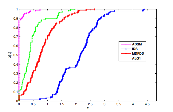
Building upon the performance profile established by Dolan and Mor\(\acute{e}\) [25], Figures 1–3 provide a comprehensive overview of the performance and efficiency of the ADSM, IDS, MDFDD, and ALG1 methods. For each solver \(s\) and problem \(p\), the performance ratio is defined as \[r_{p,s} = \frac{t_{p,s}}{\min_{s\in S}t_{p,s}}, \tag{50}\] where \(t_{p,s}\) denotes the computational effort required by solver \(s\) to solve problem \(p\). The cumulative distribution function \[p_s(\tau) = \frac{1}{n_p}\,\mathrm{card}\{p\in P:r_{p,s}\leq \tau\} \tag{51}\] represents the probability that solver \(s\) performs within a factor \(\tau\) of the best solver. In particular, \(p_s(1)\) gives the fraction of problems for which solver \(s\) is the best, while the behavior of \(p_s(\tau)\) as \(\tau\) increases reflects the robustness of the solver.
Figure 1 presents the performance profile with respect to the number of iterations. Within the interval \(0\leq \tau\leq 5\), ADSM clearly dominates the other methods. It attains the highest value of \(p(\tau)\) near \(\tau=1\), indicating that it solves the largest proportion of test problems using the minimum number of iterations. Its curve rises steeply and approaches full robustness at relatively small values of \(\tau\).
ALG1 ranks second and demonstrates competitive behavior, although its performance remains slightly below that of ADSM for small \(\tau\). MDFDD exhibits moderate efficiency, requiring larger performance ratios before reaching comparable probability levels. IDS shows the slowest growth of \(p(\tau)\) and therefore requires more iterations relative to the best-performing solver.
Figure 2 shows the performance profile based on the number of function evaluations, with \(\tau\) ranging from 0 to 7. ADSM again achieves the highest \(p(\tau)\) at \(\tau=1\), demonstrating superior efficiency in terms of function evaluations. Since function evaluation is often the dominant computational cost in large-scale optimization, this result highlights the practical advantage of ADSM. ALG1 remains highly competitive and closely follows ADSM across increasing values of \(\tau\). IDS ranks third, while MDFDD exhibits the weakest performance in this metric. Notably, MDFDD begins to show significant probability growth only at larger \(\tau\) values, indicating that it generally requires substantially more function evaluations.
Figure 3 presents the performance profile based on CPU time in seconds, with \(0\leq \tau\leq 6\). ADSM consistently attains the largest \(p(\tau)\) values for small performance ratios, indicating that it is most frequently the fastest solver. ALG1 again ranks second and shows competitive time efficiency.
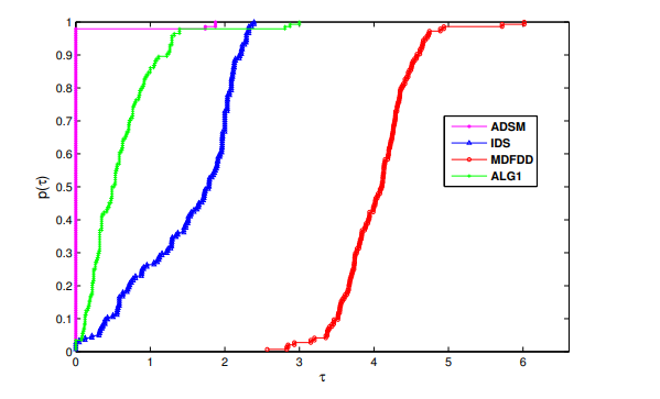
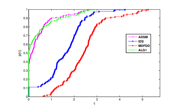
IDS demonstrates moderate performance, whereas MDFDD requires larger \(\tau\) values before reaching comparable probability levels. Although all methods approach full robustness as \(\tau\) increases, ADSM achieves this level more rapidly.
Across all three performance measures, namely iterations (\(0\leq \tau\leq 5\)), function evaluations (\(0\leq \tau\leq 7\)), and CPU time (\(0\leq \tau\leq 6\)), ADSM consistently achieves the highest probability of being the best solver, \(p(1)\), exhibits the fastest growth in \(p(\tau)\), and reaches full robustness at smaller performance factors compared with the competing methods. ALG1 demonstrates stable and competitive behavior, ranking second overall. IDS provides moderate performance, while MDFDD shows comparatively weaker efficiency, particularly in function evaluations and CPU time. These results confirm that ADSM is the most efficient and robust solver among the four methods for the tested large-scale unconstrained optimization problems.
This section discusses the motion control problem arising in two-joint planar robotic manipulators. Since (1) is equivalent to the global optimization Problem (4), Algorithm 2 can be applied to solve the resulting nonlinear system.
According to [26], the discrete-time kinematic equation of a two-joint planar manipulator at the position level is given by \[\label{mc1} \varphi(\theta_k)=u_k, \tag{52}\] where \(\varphi(\cdot)\) denotes the nonlinear forward kinematic mapping.
The kinematic mapping has the form \[\label{mc2} \varphi(\theta) = \begin{bmatrix} a_1+a_2\\ b_1+b_2 \end{bmatrix}, \tag{53}\] where \[a_1=l_1\cos(\theta_1), \qquad a_2=l_2\cos(\theta_1+\theta_2),\] and \[b_1=l_1\sin(\theta_1), \qquad b_2=l_2\sin(\theta_1+\theta_2).\] Here, \(l_1\) and \(l_2\) denote the lengths of the first and second links, respectively. The vector \[\theta_k=[\theta_1,\theta_2]^T\in\mathbb{R}^2\] represents the joint angles, while \[\varphi(\theta_k)\in\mathbb{R}^2\] denotes the position of the end effector.
At any time instant \(t_k\in[0,t_f]\), the motion control objective can be formulated as the minimization problem \[\label{mc3} \min_{u_k\in\mathbb{R}^2} \frac{1}{2}\|u_k-u_{dk}\|^2, \tag{54}\] where \(t_f\) denotes the total task duration and \(u_{dk}\) represents the desired trajectory at time \(t_k\).
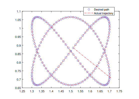
Following [27], the link lengths are chosen as \(l_1=l_2=1\). A Lissajous curve is used as the desired trajectory of the end effector: \[\label{mc4} u_{dk} = \begin{bmatrix} \frac{3}{2}+\frac{1}{5}\sin\!\left(\frac{2\pi t_k}{5}\right)\\[2mm] \frac{\sqrt{3}}{2}+\frac{1}{5}\sin\!\left(\frac{3\pi t_k}{5}\right) \end{bmatrix}. \tag{55}\]
In the motion control task, the aim is to drive the end effector of the manipulator to track the desired trajectory \(u_{dk}\). This requirement leads to the optimization problem (54). However, the end-effector position \(u_k\) is determined by the forward kinematics (52). Substituting (52) into (54), we obtain
\[\label{opt_theta} \min_{\theta_k\in\mathbb{R}^2} \frac{1}{2}\|\varphi(\theta_k)-u_{dk}\|^2. \tag{56}\]
Define the merit function \[\mathfrak{h}(\theta_k) = \frac{1}{2}\|\varphi(\theta_k)-u_{dk}\|^2.\] Minimizing (56) is equivalent to solving the nonlinear equation \[\label{motion_F} \mathfrak{F}(\theta_k) = \varphi(\theta_k)-u_{dk} = 0, \tag{57}\] where \(\mathfrak{F}:\mathbb{R}^2\rightarrow\mathbb{R}^2\) represents the residual mapping. Therefore, Algorithm 2 is applied by setting \[s_k=\theta_k,\] and \[\mathfrak{F}(s_k) = \mathfrak{F}(\theta_k) = \varphi(\theta_k)-u_{dk}.\]
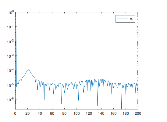
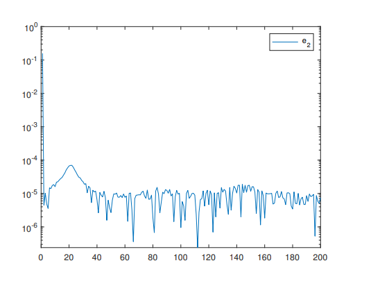
The algorithm iteratively updates \(\theta_k\) until the stopping criterion \[\label{stop_motion} \|\mathfrak{F}(\theta_k)\| \leq 10^{-5} \tag{58}\] is satisfied. The error plots reported in the numerical experiments correspond to the residual norm \(\|\mathfrak{F}(\theta_k)\|\), which represents the tracking error between the actual end-effector position \(\varphi(\theta_k)\) and the desired trajectory \(u_{dk}\).
We established the following parameters for this experiment: \[\omega_1=\omega_2=10^{-4}, \qquad q=10^{-4}, \qquad r=0.3, \qquad \chi_k=\frac{1}{(k+1)^2},\] with \(t_f=10\) seconds and the initial point \[\theta_0= \left[0,\frac{\pi}{3}\right]^T.\] Furthermore, the working interval \([0,10]\) is divided into 200 equal subintervals.
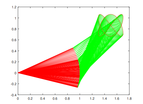
Figures 4–7 illustrate the robot trajectories generated by the ADSM algorithm. The results show that the proposed method successfully guides the end effector to follow the desired trajectory. In addition, Figures 6 and 7 present the tracking error of the end effector during the motion process. It can be observed that the error decreases rapidly and remains approximately at the level of \(10^{-5}\), which satisfies the prescribed stopping tolerance. These results confirm the effectiveness and applicability of the proposed ADSM method for solving motion control problems in robotic manipulators.
This study presents a hybridized step-size method specifically designed to tackle systems of nonlinear equations. A notable advantage of the proposed method is the use of two different line-search techniques and its derivative-free characteristic, which significantly enhances its efficiency for solving problem (1). This feature makes it particularly advantageous in scenarios where obtaining derivative information may be challenging or costly. To thoroughly evaluate the performance of the proposed method, we conducted extensive numerical comparisons using a set of large-scale test problems. The results are summarized in Tables 2–4 and visually represented in Figures 1–3. Our findings reveal that the proposed method consistently requires fewer iterations and less CPU time compared with several other established techniques in the field. Additionally, we applied the proposed method to a motion control problem involving two-joint planar robotic manipulators, demonstrating its practical applicability. The outcomes of this application are illustrated in Figures 4–7, underscoring the method’s effectiveness in real-world situations. In future work, we intend to explore the development of a two-step-size method for solving motion control problems with four degrees of freedom.
Abubakar Sani Halilu: Methodology, Software, Writing–original draft. Arunava Majumder and Mohamad Afendee Mohamed: Validation, Writing–review and editing, Supervision. Mohammed Yusuf Waziri and Sulaiman M. Ibrahim: Conceptualization, Methodology. Kabiru Ahmed and Muhammad Abdullahi: Validation, Formal analysis, Investigation.
The authors declare that there is no conflict of interest regarding the publication of this paper.