
Time-periodic parabolic equations and systems arise naturally and frequently in applied mathematics, including population dynamics, chemical reactions, heat conduction in periodic environments, and environmental modeling. The study of their time-periodic solutions is particularly significant, as these solutions characterize the long-term behavior or the steady-state conditions of systems subjected to periodic forces.
Analysis of periodic solutions to parabolic equations has a lengthy and rich history. Among the most potent tools in this field is the sub- and super-solutions method, providing a constructive framework for proving the existence of solutions lying between ordered barriers. This method was originally developed for elliptic problems by [1], and was later extended to parabolic systems by [2] and [3]. Its applicability relies crucially on the maximum principle and the inherent monotonicity properties that characterize cooperative structures. Pioneering contributions by [4] and [5] established fundamental results using topological techniques and the theory of monotone dynamical systems. The existence of weak solutions for Leray-Lions type operators was investigated in [6] using the theory of maximal monotone operators. In the context of quasi-linear problems with critical gradient growth, the existence and regularity of weak solutions using sub- and super-solution techniques were established in [7]. This study was further extended in [8] to problems with \(L^1\) data, in which a combination of truncation and sub-super solution methods yielded a solution obtained as a limit of approximations (SOLA). In the context of the Navier-Stokes equations, the existence of strong periodic solutions in 2D with non-local viscosity was established by Ferreira et al. [9].
In addition to theoretical advances, numerical techniques for periodic parabolic problems have been extensively developed. For instance, a least squares method for numerical simulation was developed in [10]. To address problems with unknown time periods, an iterative construction scheme was introduced in [11]. Alternatively, in [12], the problem was formulated as an evolution equation, proving existence via semigroup theory and fixed point theorems, and using Newton’s method for numerical simulation. It is worth noting that both the numerical studies mentioned above and the theoretical works discussed earlier mainly deal with periodic parabolic equations with continuous coefficients. In [13], the authors studied a periodic parabolic problem with singular nonlinearity involving a variable exponent. Under suitable assumptions on the exponent and the data, the authors proved the existence of nonnegative weak solutions. The discontinuous coefficient case was discussed in [14] by reformulating the periodicity condition \(u(0)=u(T)\) as the minimization of a least-squares cost functional over an admissible space of initial data. The proposed optimization-based variational framework accommodates discontinuous coefficients, yields a constructive characterization of periodic solutions suitable for numerical implementation, and provides a rigorous foundation for gradient-based iterative schemes. The techniques developed therein extend naturally to nonlinear problems, including systems with \(p(x)\)-growth conditions [15].
In this work, we consider a general class of nonlinear cooperative parabolic systems given by \[\dfrac{\partial u_i}{\partial t} – D_i \Delta u_i = f_i(t,x,u), \quad i=1,\dots,m,\] with periodicity \(T\) in time and homogeneous Neumann boundary conditions. We assume that the nonlinearities \(f_i\) satisfy Carathéodory’s conditions, guaranteeing the continuity and measurability properties necessary for the analysis. The system preserves a structure of natural order according to the cooperativity hypothesis, which requires non-negative cross-participal derivatives \(\partial f_i/\partial u_j \geq 0\) for \(i \neq j\).
The present work extends the periodic ODE systems investigated by Alaa et al. [16] to the space-dependent case. In this context, the main contributions are threefold: First, we develop a rigorous functional-analytical framework for weak periodic solutions, establishing the existence and compactness properties of periodic Green operators in a suitably adapted framework for cooperative parabolic systems with Neumann boundary conditions. Second, using the monotone iteration scheme combined with the sub- and super-solution method, we prove the existence of extremal periodic solutions under minimal hypotheses, requiring only the existence of ordered lower and upper solutions without any additional restrictions on the growth of nonlinearities. Third, a precise uniqueness criterion is derived that relates the Lipschitz constant of nonlinearity to the operator norm of the associated Green operators, thus providing a verifiable condition for uniqueness in applications. These results not only generalize the classical theory of monotone iterations to the periodic case, but also provide a set of practical tools for analyzing periodic phenomena in environmental and hydrological systems, as illustrated by their application to a model of water solute transport in porous media.
The remainder of this paper is structured as follows. §2 establishes the functional framework and develops the linear theory, including the construction of the periodic resolvent kernel as well as an analysis of its key properties. In §3, we turn to the nonlinear problem under Carathéodory-type hypotheses, employing monotone iteration techniques to prove the existence of extremal solutions. §3.4 is dedicated to the uniqueness of these solutions, where we derive a more precise criterion based on Lipschitz conditions. §3.5 is devoted to the asymptotic analysis of periodic solutions via the Poincaré map. In §3.6, we illustrate the theoretical results by applying them to a model of water-solute interaction in porous media, thus demonstrating the practical relevance of the developed framework. The numerical approximation of the coupled reaction-diffusion system from §3.6 is discussed in §4. Based on a first-order IMEX scheme with Crank-Nicolson for diffusion, we introduce an iterative approach and spatiotemporal discretization for handling periodic boundary conditions. Numerical results confirm the robustness and efficiency of this approach.
Let \(\Omega\) be an open bounded subset of \(\mathbb{R}^N\) \((N \ge 1)\), and let \(T>0\) be a given period. We introduce the following functional space \[X_{\mathrm{per}} := \Big\{ u \in C([0,T]; L^2(\Omega)) \cap L^2(0,T; H^1(\Omega)) \; : \; \partial_t u \in L^2(0,T; H^1(\Omega)’) ,\; u(0,\cdot) = u(T,\cdot) \Big\},\] endowed with the norm \[\|u\|_{X_{\mathrm{per}}} := \sup_{0\le t\le T} \|u(t,\cdot)\|_{L^2(\Omega)} + \|\nabla u\|_{L^2(Q_T)} + \Big\|\dfrac{\partial u}{\partial t}\Big\|_{L^2(0,T; H^1(\Omega)’)} ,\] where \(Q_T=]0,T[\times\Omega\). For the analysis of the proposed system, we define the product space \[\mathcal{X}^m_{\mathrm{per}} = \underbrace{X_{\mathrm{per}} \times X_{\mathrm{per}} \times \dots \times X_{\mathrm{per}}}_{m\text{-times}},\] equipped with the following norm \[\|u\|_{\mathcal{X}^m_{\mathrm{per}}} = \sum\limits_{i=1}^m\|u_i\|_{X_{\mathrm{per}}} \quad \text{ where } u=(u_1,…,u_m).\]
We introduce a component-wise order on \(\mathcal{X}^m_{\mathrm{per}}\) by defining, for \(u, v \in \mathcal{X}^m_{\mathrm{per}}\), \[u \leq v \Longleftrightarrow u_i \leq v_i \qquad \text{ for all } i=1,\cdots,m,\] where, for each component, the inequality \(u_i \le v_i\) holds pointwise almost everywhere in \(Q_T\), i.e., \(u_i(t,x) \leq v_i(t,x)\) for almost every \(t,x \in Q_T\).
Remark 1. The function space \(\mathcal{X}^m_{\mathrm{per}}\) possesses the following fundamental properties:
\(\mathcal{X}^m_{\mathrm{per}}\) is a Banach space.
The embedding \(\mathcal{X}^m_{\mathrm{per}} \hookrightarrow C\left([0,T];L^2(\Omega)^m\right)\) is continuous.
For any \(u \in \mathcal{X}^m_{\mathrm{per}}\), the time derivative \(\partial_t u\) is understood in the weak sense. Specifically, for each component \(u_i\), we have \[\int_0^T\langle \partial_t u, \varphi \rangle = – \sum\limits_{i=1}^m\int_{Q_T} u_i \, \partial_t \varphi_i \, dx \, dt, \qquad \forall\, \varphi \in H_{\mathrm{per}}^1(0,T; L^2(\Omega)^m),\] where \(H_{\mathrm{per}}^1(0,T; L^2(\Omega)^m)=\{\varphi \in L^2(0,T; L^2(\Omega)^m),\partial_t\varphi\in L^2(0,T; L^2(\Omega)^m),\varphi(0,\cdot) = \varphi(T,\cdot)\}\).
We first recall the linear \(T\)-periodic parabolic problem \[\left\{ \begin{array}{ll} \dfrac{\partial u}{\partial t} – D\, \Delta u = \sigma, & \text{in } Q_T := (0,T)\times\Omega, \\[1ex] u(0,\cdot) = u(T,\cdot), & \text{in } \Omega, \\[1ex] \dfrac{\partial u}{\partial \nu} = 0, & \text{on } \Sigma_T := (0,T)\times\partial\Omega, \end{array} \right. \tag{1} \] where \(D>0\) is a constant diffusion coefficient, and \(\sigma \in L^2(Q_T)\) is assumed to be \(T\)-periodic in time.
Lemma 1. Let \(D>0\) and let \(\sigma \in L^2(Q_T)\) be \(T\)-periodic in time. Then the following claims hold:
(i) Problem 1 admits a unique weak \(T\)-periodic solution \(u \in X_{\mathrm{per}}\) given by \[u(t,x) = \int_0^T \int_{\Omega} K_{\mathrm{per}}^D(t,x;\tau,\xi)\, \sigma(\tau,\xi)\, d\xi\, d\tau = (K_D\sigma)(t,x),\] where \(K_{\mathrm{per}}^D(t,x;\tau,\xi)\) denotes the periodic Green’s function associated with the linear problem (1).
(ii) The operator \[K_D: L^2(Q_T) \to X_{\mathrm{per}} \hookrightarrow L^2(Q_T),\] is linear and continuous, namely \[\|K_D \sigma\|_{X_{\mathrm{per}}} \le C \|\sigma\|_{L^2(Q_T)},\] where \(C=C(D,T,\Omega)\).
Moreover, since the embedding of \(X_{\mathrm{per}}\) into \(L^2(Q_T)\) is compact, the operator \(K_D: L^2(Q_T) \to L^2(Q_T)\) is compact.
(iii) The operator \(K_D\) is positive in the sense that if \(f \in L^2(Q_T)\) satisfies \(f \geq 0\) a.e in \(Q_T\), then \(K_D f\geq 0\) a.e in \(Q_T\).
(iv) For every \(\sigma \in L^2(Q_T)\), the function \(u=K_D(\sigma)\) is the unique element of \(X_{\mathrm{per}}\) satisfying (1).
Definition 1. Let \(D>0\) and \(\sigma\in L^2(Q_T)\) be a T-periodic function. A measurable function \(u : Q_T \to \mathbb{R}\) is a weak \(T\)-periodic solution to (1) if the following conditions are satisfied \(u \in X_{\mathrm{per}}\) and \[\int_0^T \left\langle \dfrac{\partial u}{\partial t}, \varphi \right\rangle \, dt + D \int_{Q_T} \nabla u \cdot \nabla \varphi \, dx\,dt = \int_{Q_T} \sigma \varphi dxdt,\] for all test function \(\varphi \in L^2(0,T;H^1(\Omega))\).
Lemma 2. Let \(D>0\) and \(\sigma \in L^2(Q_T)\) be a \(T\)-periodic function. Then \(u \in X_{\mathrm{per}}\) is a weak \(T\)-periodic solution of problem (1) if and only if, \[u(t,x) = \int_0^T \int_{\Omega} K_D(t,s,x,y)\, \sigma(s,y)\, dy\, ds,\] where \(K_D\) denotes the periodic Green’s kernel associated with the linear problem.
We now consider the nonlinear periodic parabolic system formulated as follows \[\left\{ \begin{array}{ll} \dfrac{\partial u_i}{\partial t} – D_i\, \Delta u_i = f_i(t,x,u_1,\dots,u_m), & \text{in } Q_T := (0,T) \times \Omega, \\[1ex] \dfrac{\partial u_i}{\partial \nu} = 0, & \text{on } \Sigma_T := (0,T) \times \partial\Omega, \\[1ex] u_i(0, \cdot) = u_i(T, \cdot), & \text{in } \Omega, \end{array} \right. \qquad i = 1,\dots,m . \tag{2} \] where, for each \(i=1, \ldots, m\), the function \(f_i: Q_T \times C \rightarrow \mathbb{R}\), with \(C \subset \mathbb{R}^m\) a bounded open set, satisfies the Carathéodory conditions, thereby ensuring that the associated Nemytskii operator is well-defined on the appropriate function space.
(H1) (Measurability and periodicity). For each \(u\in C\), the function \((t,x)\longmapsto f_i(t,x,u)\) is Lebesgue-measurable on \(Q_T\), \(T\)-periodic with respect to \(t\), and belongs to \(L^2(Q_T)\).
(H2) (Local \(\mathcal{C}^1\) regularity). For a.e \((t,x)\in Q_T\), the function \(u \longmapsto f_i(t,x,u)\) is of class \(\mathcal{C}^1(C)\) .
(H3) (Cooperativity). For all \(u\in C, j\neq i\) and a.e \((t,x)\in Q_T\), \(\dfrac{\partial f_i}{\partial u_j}(t,x,u) \ge 0\).
(H4) (Local boundedness). There exists a function \(g\in L^2(Q_T)\) such that, for each \(i=1,\dots,m\), \(|f_i(t,x,u)|\le g(t,x)\), for a.e. \((t,x)\in Q_T\) and for all \(u\in C\).
Under assumptions (H1)–(H4), for every \(u \in C\) the nonlinear terms satisfy \[f_i(\cdot,\cdot,u) \in L^2(Q_T), \qquad i=1,\dots,m.\]
Consequently, the associated Green operators \[K_{D_i} : L^2(Q_T) \to X_{\mathrm{per}}, \quad i=1,\cdots,m,\] are well defined and continuous on these right-hand sides.
Definition 2 (Weak \(T\)–periodic solution). Suppose that (H1)–(H4) hold. A function \(u=(u_1,\cdots,u_m)\in \mathcal{X}^m_{\mathrm{per}}\) with \(u(t,x)\in C\) for a.e \((t,x)\in Q_T\) is called a weak \(T\)-periodic solution of (2) if for all \(i=1,\cdots,m\) and for all test function \(\varphi \in L^2(0,T;H^1(\Omega))\), \[\displaystyle\int_0^T \left\langle \dfrac{\partial u_i}{\partial t}, \varphi \right\rangle \, dt +D_i \int_{Q_T} \nabla u_i \cdot \nabla \varphi \, dx\,dt = \int_{Q_T} f_i(t,x,u(t,x)) \varphi dxdt,\] which is equivalent to \[u_i(t,x)=\displaystyle\int_0^T \int_{\Omega} K_{D_i}(t,s,x,y)\, f_i(s,y,u(s,y))\, dy\, ds,\]
In this section, we work in the ordered Banach space \(\mathcal{X}^m_{\mathrm{per}}\) endowed with the componentwise order introduced above.
Definition 3 (\(T\)-periodic sub- and super-solutions). Suppose (H1)–(H4) hold. A vector \(w=(w_1,\dots,w_m)\in \mathcal{X}_{\mathrm{per}}^m\) is called a \(T\)-periodic subsolution of system (2) if, for each \(i=1,\ldots,m\), and all \(\varphi\in L^2(0,T;H^1(\Omega))\) with \(\varphi\geq 0\) a.e., \[\int_0^T\Bigl\langle \dfrac{\partial w_i}{\partial t},\varphi\Bigr\rangle\,dt + D_i\int_{Q_T}\nabla w_i\cdot\nabla\varphi\,dx\,dt \leq \int_{Q_T} f_i(t,x,w)\,\varphi\,dx\,dt. \tag{3} \]
Similarly, \(\hat{w}=(\hat{w}_1,\dots,\hat{w}_m)\in \mathcal{X}_{\mathrm{per}}^m\) is called a \(T\)-periodic supersolution of (2) if, for each \(i=1,\ldots,m\), and all \(\varphi\in L^2(0,T;H^1(\Omega))\) with \(\varphi\ge 0\) a.e., \[\int_0^T\Bigl\langle \dfrac{\partial \hat{w}_i}{\partial t},\varphi\Bigr\rangle\,dt + D_i\int_{Q_T}\!\nabla \hat{w}_i\cdot\nabla\varphi\,dx\,dt \geq \int_{Q_T} f_i(t,x,\hat{w})\,\varphi\,dx\,dt. \tag{4} \]
The pair \((w,\hat{w})\) is called an ordered pair of sub and super-solutions if \(w_i(t,x)\leq \hat{w}_i(t,x)\) for a.e. \((t,x)\in Q_T\) and each \(i=1,\dots,m\).
Remark 2. The weak sub/supersolution conditions (3)–(4) imply the corresponding kernel form inequalities: if \(w\in\mathcal{X}_{\mathrm{per}}^m\) satisfies (3), then the positivity of \(K_{D_i}\) (Lemma 1 (iii)) yields \[w_i(t,x) \leq \left(K_{D_i}(f_i(\cdot,\cdot,w))\right)(t,x) \quad \text{for a.e. } (t,x)\in Q_T. \tag{5} \]
Analogously, for supersolutions \[\hat w_i(t,x) \geq \left(K_{D_i}(f_i(\cdot,\cdot,\hat w))\right)(t,x) \quad \text{for a.e. } (t,x)\in Q_T, \tag{6} \] (see [5]). In particular, (5) states precisely that \(w \le \mathcal{T}(w)\) componentwise a.e., while (6) yields \(\hat{w} \ge \mathcal{T}(\hat{w})\) componentwise a.e., where \(\mathcal{T}\) denotes the fixed-point operator introduced below. These kernel-form inequalities are those directly employed in the subsequent proofs.
For an ordered pair of \(T\)-periodic sub- and super-solutions \((w,\hat w)\), we define the order interval in \(L^2(Q_T)^m\): \[:=\Bigl\{ u=(u_1,\dots,u_m)\in L^2(Q_T)^m \;\Big|\; w_i\le u_i\le \hat{w}_i\ \text{ a.e. in }Q_T,\ i=1,\dots,m \Bigr\}. \tag{7} \]
This is a closed, bounded, convex subset of \(L^2(Q_T)^m\).
We now introduce the key structural hypothesis controlling the diagonal derivatives of \(f_i\) inside the order interval.
(H5) (Diagonal monotonicity). For each \(i=1,\dots,m\), \(\dfrac{\partial f_i}{\partial u_i}(t,x,u)\ge 0, \quad \text{for a.e. } (t,x)\in Q_T,\ \forall u\in [w,\hat w]\).
Under assumptions (H1)–(H5), we can define the nonlinear operator \[\mathcal{T}: [w,\hat w]\longrightarrow L^2(Q_T)^m, \tag{8} \] componentwise by \[\mathcal{T}(u) :=\left((\mathcal{T}u)_1,\dots,(\mathcal{T}u)_m\right),\] where, for each \(i=1,\dots,m\), \[(\mathcal{T}u)_i := K_{D_i}\left(f_i(\cdot,\cdot,u)\right).\]
By (H4), \(f_i(\cdot,\cdot,u)\in L^2(Q_T)\), and \(K_{D_i}:L^2(Q_T)\to X_{\mathrm{per}}\) is bounded (Lemma 1(ii)), then \(\mathcal{T}(\)u\()\) belongs to \(\mathcal{X}^m_{\mathrm{per}} \subset L^2(Q_T)^m\) for all \(u\in[w,\hat{w}]\). In the following, we aim to show that \(\mathcal{T}\) maps the interval onto itself and is compact on \(L^2(Q_T)^m\).
Lemma 3 (Order preservation and invariance of the interval). Assume (H1)–(H4) and (\(H_5\)) hold, and let \((w,\hat w)\) be an ordered pair of weak sub- and super-solutions of (2) in the sense of Definition 3. Then the following statements hold
(i) \(\mathcal{T}\) maps the interval into itself, \[\mathcal{T}([w,\hat w])\subset [w,\hat w].\]
(ii) \(\mathcal{T}\) is order preserving: if \(u,v \in [w,\hat w]\) with \(u \leq v\) a.e., then \(\mathcal{T}(u) \leq \mathcal{T}(v)\) a.e. in \(Q_T\).
(iii) \(\mathcal{T}\) is compact and continuous.
Proof.
(Invariance of \([w, \hat w]\)). Let \(u\in [w,\hat w]\) be fixed. We prove \(\mathcal{T}(u)\in [w,\hat w]\), namely \[w_i \le (\mathcal{T}(u))_i \le \hat w_i \quad \text{a.e. in } Q_T, \qquad i=1,\dots,m.\]
By definition, \[(\mathcal{T}(u))_i= K_{D_i}\left(f_i(\cdot,\cdot,u)\right).\]
Since \(w\) is a sub-solution of the nonlinear system (2), Lemma 1-iii) yields \[w_i \le K_{D_i}\left(f_i(\cdot,\cdot,w)\right) \quad \text{a.e. in } Q_T.\]
Hence, \[(\mathcal{T}(u))_i – w_i \ge K_{D_i}\left(f_i(\cdot,\cdot,u) – f_i(\cdot,\cdot,w)\right).\]
Set \(\delta(t,x):=u(t,x)-w(t,x)\). Since \(u\in[w,\hat w]\), we have \(\delta_j(t,x)\ge 0\) for all \(j=1,\dots,m\) and for a.e. \((t,x)\in Q_T\).
By hypothesis \((H_2)\) and the integral form of the mean value theorem, we can write \[f_i(t,x,u)-f_i(t,x,w)=\sum_{j=1}^m \delta_j(t,x)
\int_0^1\dfrac{\partial f_i}{\partial u_j}
\left(t,x,\,w+\theta\delta\right)\,d\theta\ge 0,\quad \text{a.e. in } Q_T.\] \[\begin{aligned}
f_i(t,x,u)-f_i(t,x,w)=\int_0^1 \sum_{\substack{j=1\\ j\neq i}}^{m}\dfrac{\partial f_i}{\partial u_j}\left(t,x,\,w+\theta\delta\right)\,\delta_j\,d\theta + \int_0^1\dfrac{\partial f_i}{\partial u_i}\left(t,x,\,w+\theta\delta\right)\,\delta_i\,d\theta.
\end{aligned}\]
By the cooperativity assumption \((H_3)\), the monotonicity assumption \((H_5)\),and the fact that \(\delta_j\ge 0\) a.e. in \(Q_T\), all terms are nonnegative; thus, we obtain \[f_i(t,x,w)\le f_i(t,x,u) \quad \text{for a.e. } (t,x)\in Q_T.\]
By \((H_4)\), \(f_i(\cdot,\cdot,u)\in L^2(Q_T)\), and since \(K_{D_i}\) is positive and order-preserving, applying \(K_{D_i}\) to the above inequality yields \[K_{D_i}\left(f_i(\cdot,\cdot,w)\right) \le K_{D_i}\left(f_i(\cdot,\cdot,u)\right) \quad \text{a.e. in } Q_T.\]
From the sub-solution condition (5), \(w_i \le K_{D_i}(f_i(\cdot,\cdot,w))\) . Combining these two inequalities yields \[w_i \leq K_{D_i}\left(f_i(\cdot,\cdot,u)\right) = \left(\mathcal{T}(u)\right)_i \quad \text{a.e.}.\]
Applying the same argument to the pair \((u,\hat w)\) gives \[K_{D_i}\left(f_i(\cdot,\cdot,u)\right) \le K_{D_i}\left(f_i(\cdot,\cdot,\hat w)\right) \quad \text{a.e. in } Q_T.\]
Using the supersolution condition (6), we obtain \[\left(\mathcal{T}(u)\right)_i \leq K_{D_i}\left(f_i(\cdot,\cdot,\hat{w})\right) \leq \hat{w}_i \quad \text{a.e.}.\]
Consequently, \[w_i \le (\mathcal{T}(u))_i \le \hat w_i \quad \text{a.e. in } Q_T, \qquad i=1,\dots,m.\]
This proves that \(\mathcal{T}(u)\in[w,\hat w]\) for every \(u\in[w,\hat w]\). Hence \[\mathcal{T}([w,\hat w])\subset [w,\hat w].\]
(ii) (The operator \(\mathcal{T}\) preserves the order). Let \(u\le v\) and set \(\delta:=v-u\ge 0\). By the integral Taylor formula and assumptions \((H_2)\), \((H_3)\) and \((H_5)\), we get \[f_i(\cdot,\cdot,v)-f_i(\cdot,\cdot,u)\ge 0 \quad \text{a.e. in }Q_T.\] for each \(i=1,\cdots,m\).
Since each Green operator \(K_{D_i}\) is positive and order-preserving, we obtain \[K_{D_i}\left(f_i(\cdot,\cdot,u)\right) \le K_{D_i}\left(f_i(\cdot,\cdot,v)\right) \quad \text{a.e. in }Q_T.\]
Applying this inequality componentwise yields \(\mathcal{T}(u)\le \mathcal{T}(v)\).
(iii) (Compactness and continuity of \(\mathcal{T}\)). We start by proving the continuity. Let \((u^n)_{n\in\mathbb{N}} \subset [w,\hat w]\) be such that \(u^n\to u\) in \(L^2(Q_T)^m\). Then up to a subsequence, \[u^n(t,x)\to u(t,x) \quad \text{for a.e. }(t,x)\in Q_T.\]
By the Carathéodory regularity assumption \((H_1)\), this implies \[f_i(t,x,u^n(t,x)) \to f_i(t,x,u(t,x)) \quad \text{for a.e. }(t,x)\in Q_T.\]
Moreover, by the growth condition \((H_4)\), there exists \(g\in L^2(Q_T)\) such that \[|f_i(t,x,u^n(t,x))|\le g(t,x) \quad \text{for a.e. }(t,x)\in Q_T \text{ and all } n.\]
Therefore, by appling the dominated convergence theorem, one can get \[f_i(\cdot,\cdot,u^n)\to f_i(\cdot,\cdot,u) \quad \text{in } L^2(Q_T).\]
Finally, since \(K_{D_i}:L^2(Q_T)\to X_{\mathrm{per}}\) is linear and continuous, we obtain \[K_{D_i}\left(f_i(\cdot,\cdot,u^n)\right) \to K_{D_i}\left(f_i(\cdot,\cdot,u)\right) \quad \text{in } L^2(Q_T),\]
Hence \(\mathcal{T}(u^n)\to \mathcal{T}(u)\) in \(L^2(Q_T)^m\), proving that the operator is continuous on \([w,\hat w]\).
We now prove that \(T\) is compact. Let \(\{u^n\}\subset [w,\hat w]\) be an arbitrary sequence. By definition of the order interval, we have \[w_i(t,x)\le u_i^n(t,x)\le \hat w_i(t,x) \quad \text{for a.e. }(t,x)\in Q_T,\ \forall n,\ \forall i.\]
The growth condition \((H_4)\) ensures the existence of a function \(g\in L^2(Q_T)\) such that \[\|f_i(\cdot,\cdot,u^n)\|_{L^2(Q_T)} \le \|g\|_{L^2(Q_T)}, \quad \text{ for all } i=1,\dots,m.\]
Therefore \(\{f_i(\cdot,\cdot,u^n)\}\) is bounded in \(L^2(Q_T)\).
Since each Green operator \(K_{D_i}:L^2(Q_T)\to X_{\mathrm{per}}\) is linear and continuous (Lemma 1(ii)), the sequence \(\{K_{D_i}(f_i(\cdot,\cdot,u^n))\}\) is bounded in \(X_{\mathrm{per}}\). Since the embedding \(X_{\mathrm{per}}\hookrightarrow L^2(Q_T)\) is compact ([19]), one can extract a subsequence (still denoted by \(n\)) such that there exist \(U_i \in L^2(Q_T)\), \(i = 1,\ldots,m\), \[K_{D_i}\left(f_i(\cdot,\cdot,u^n)\right)\to U_i \quad \text{ strongly in } L^2(Q_T), \ i=1,\dots,m.\]
Consequently, \[\mathcal{T}(u^n)\to (U_1,\dots,U_m) \quad \text{in } L^2(Q_T)^m,\] which shows that \(T([w,\hat w])\) is relatively compact in \(L^2(Q_T)^m\). Therefore, \(\mathcal{T}\) is compact.
\(\square\)
Theorem 1. Assume (H1)–(H5). Suppose that the system (2) admits a pair of weak \(T\)-periodic sub- and super-solution \(w,\hat w \in L^2(Q_T)^m\) in the sense of Definition 3. Then there exists at least one weak \(T\)-periodic solution \(u \in \mathcal{X}^m_{\mathrm{per}}\) of (2) such that \[w(t,x) \leq u(t,x) \leq \hat w(t,x) \quad \text{ a.e } (t,x) \in Q_T.\]
Proof. Let \(\mathcal{T}\) be the operator defined in (8). By Lemma 3 we know that \(\mathcal{T}\) is order preserving, continuous, compact and leaves the interval \([w,\hat w]\) invariant.
Define the monotone sequence \((u^n)_{n\ge 0} \subset [w,\hat w]\) by \[u^0:=w, \quad u^{n+1}:= \mathcal{T}(u^n), \ n \geq 0.\]
By Lemma 3 \((i)\) we have \(u^n\in [w,\hat w]\) for all \(n\geq 0\).
We prove by induction that the sequence is monotone increasing. For \(n=0\), the subsolution property \(w_i \leq K_{D_i}(f_i(\cdot,\cdot,w))\) a.e. implies \(u^0 \leq \mathcal{T}(u^0)=u^1\) a.e. Assume \(u^{n-1}\leq u^n\) a.e. for some \(n\ge 1\). Then, by Lemma 3(ii), \[u^n = \mathcal{T}(u^{n-1}) \leq \mathcal{T}(u^n) = u^{n+1} \quad \text{a.e.}.\]
By induction, \(w = u^0 \le u^1 \le u^2 \le \cdots \le \hat{w}\) a.e. in \(Q_T\).
The sequence \((u^n)\) is monotone increasing and bounded above by \(\hat{w}\in L^2(Q_T)^m\). By the Monotone Convergence Theorem applied componentwise in \(L^2(Q_T)\), there exists a limit function \(u\in L^2(Q_T)^m\) such that \[u^n(t,x) \nearrow u(t,x) \quad \text{ a.e.\ in } Q_T, \quad u^n \to u \quad \text{ in } L^2(Q_T)^m.\]
In particular \(w \le u \leq \hat{w}\) a.e., whence \(u\in [w,\hat{w}]\).
Moreover, the entire sequence \(\{u^n : n\ge 1\}\) lies in \(\mathcal{T}([w,\hat{w}])\), which is relatively compact in \(L^2(Q_T)^m\) by Lemma 3 (iii). Consequently, there exists a subsequence \(\{u^{n_k}\}\) such that \(u^{n_k} \to u\) in \(L^2(Q_T)^m\). Since the sequence \(\{u^n\}\) is monotone, the full sequence satisfies \[u^n \to u \quad \text{ in } L^2(Q_T)^m.\]
By the continuity of \(\mathcal{T}\) on \(L^2(Q_T)^m\) (Lemma 3(iii)), we have \[\mathcal{T}(u^n) \xrightarrow{} \mathcal{T}(u) \quad \text{ in } L^2(Q_T)^m.\]
Since \(u^{n+1}=\mathcal{T}(u^n)\) and \(u_{n+1}\to u\) in \(L^2(Q_T)^m\), uniqueness of limits gives \(u=\mathcal{T}(u)\). Hence, \[u_i=K_{D_i}(f_i(.,.,u)) \quad \text{ a.e. in }Q_T, \quad i=1,\dots,m.\]
By virtue of (H4), we have \(f_i(\cdot,\cdot,u)\in L^2(Q_T)\), and the boundedness of \(K_{D_i}:L^2(Q_T)\to X_{\mathrm{per}}\) (Lemma 1(ii)) implies \(u\in\mathcal{X}^m_{\mathrm{per}}\). Consequently, \(u\) is a weak \(T\)-periodic solution of (2) in the sense of Definition 2, satisfying \(w\le u\le\hat{w}\) a.e. \(\square\)
Assuming the same conditions, the monotone scheme produces extremal periodic solutions within the order interval.
Theorem 2 (Minimal and maximal \(T\)-periodic weak solutions). Under the hypotheses of Theorem 1, define the sequences \[u^{0} := w, \quad u^{n+1} := \mathcal{T} u^{n}, \quad v^{0} := \hat w, \quad v^{n+1} := \mathcal{T} v^{n}, \quad n\geq 0.\]
Then the following statements hold
1. The sequence \((u^{n})_{n\geq 0}\) is monotone increasing in \([w,\hat w]\) and converges in \(L^2(Q_T)^m\) to a weak \(T\)-periodic solution \(u_*\in\mathcal{X}_{\mathrm{per}}^m\) of (2) satisfying \(w \leq u_* \leq \hat w.\)
2. The sequence \((v^{n})_{n\geq 0}\) is monotone decreasing in \([w,\hat w]\) and converges in \(L^2(Q_T)^m\) to a weak \(T\)-periodic solution \(u^*\in\mathcal{X}_{\mathrm{per}}^m\) of (2) satisfying \(w \leq u* \leq \hat w.\)
3. \(u_*\le u^*\) a.e. in \(Q_T\). Moreover, the function \(u_*\) is the minimal and \(u^*\) is the maximal \(T\)-periodic solution of (2) in the order interval \([w,\hat w]\); i.e., if \(\tilde{u}\) is any other \(T\)-periodic solution satisfying \(w \leq \tilde{u} \leq \hat w\), then \(u_* \leq \tilde{u} \leq u^*\) a.e. in \(Q_T\).
Proof. The monotone increasing property and \(L^2(Q_T)^m\)-convergence of \((u^n)\) to a fixed point \(u_*\in\mathcal{X}^m_{\mathrm{per}}\) with \(w\le u_*\le\hat{w}\) are established in the proof of Theorem 1. Consequently, \(u_*\) is a \(T\)-periodic solution of (2).
We prove that \((v^n)\) is monotone decreasing. For \(n=0\), the supersolution property of \(\hat{w}\) yields \(\hat{w}_i \ge K_{D_i}(f_i(\cdot,\cdot,\hat{w}))\) a.e., i.e., \(v^0=\hat{w}\ge\mathcal{T}(\hat{w})=v^1\) a.e. Assume \(v^{n-1}\ge v^n\) a.e. for some \(n\geq 1\). Then, by Lemma 3(ii), we have \[v^n = \mathcal{T}(v^{n-1})\geq\mathcal{T}(v^n)=v^{n+1} \quad \text{ a.e.} .\]
By induction, we get \(w \leq v^{n+1}\leq v^n \leq \hat{w}\) a.e. for all \(n\), where the lower bound \(v^n \geq w\) is derived from Lemma 3(i). Thus, \((v^n)\) is a monotone decreasing sequence and bounded below by \(w\in L^2(Q_T)^m\). Applying the Monotone Convergence Theorem componentwise yields a limit function \(u^*\in L^2(Q_T)^m\) satisfying \(w\le u^*\le\hat{w}\) a.e., and \[v^n \searrow u^* \quad \text{a.e. and in } L^2(Q_T)^m.\]
Following the argument of Theorem 1, the continuity of \(\mathcal{T}\) implies \(u^*=\mathcal{T}(u^*)\); hence \(u^*\in\mathcal{X}^m_{\mathrm{per}}\) is a weak \(T\)-periodic solution of (2).
Let \(\tilde{u}\in [w,\hat{w}]\) be any weak \(T\)-periodic solution of (2), i.e., any fixed point of \(\mathcal{T}\) in \([w,\hat{w}]\) satisfying \(\tilde{u}=\mathcal{T}(\tilde{u})\) and \(w\le\tilde{u}\leq\hat{w}\) a.e.
By construction of the sequences, we have \[w=u^{0} \le \tilde{u} \le v^{0}=\hat w.\]
Assume \(u^{n} \le \tilde{u} \le v^{n}\) for some \(n\ge0\). By the order-preserving property of \(\mathcal{T}\) (Lemma 3(ii)) and the fact that \(\tilde{u}\) is a fixed point, we obtain \[u^{n+1} = \mathcal{T}(u^n) \leq \mathcal{T}(\tilde{u}) = \tilde{u} \leq \mathcal{T}(v^n) = v^{n+1} \quad \text{a.e.}.\]
By induction, the inequality \(u^{n} \le \tilde{u} \le v^{n}\) holds for all \(n\in\mathbf{N}\).
Passing to the limit \(n\to\infty\) and using the convergences \(u^n\to u_*\) and \(v^n\to u^*\) in \(L^2(Q_T)^m\), we obtain \[u_* \leq \tilde{u} \leq u^* \quad \text{a.e. in } Q_T ,\] for any weak \(T\)-periodic solution \(\tilde{u}\in[w,\hat{w}]\) of (2). In particular, taking \(\tilde{u}=u^*\) yields \(u_*\leq u^*\), while the choice \(\tilde{u}=u_*\) gives the reverse inequality. Consequently, \(u_*\) and \(u^*\) are, respectively, the minimal and maximal \(T\)-periodic solutions of the system within the order interval \([w,\hat{w}]\). \(\square\)
For the uniqueness (and stability) within the order interval, we add the following pointwise Lipschitz condition.
(H6) (Pointwise Lipschitz condition on the order interval). There exists a constant \(L>0\) such that, for a.e. \((t,x)\in Q_T\) and all \(r,s\in\mathbb{R}^m\) satisfying \(w(t,x)\leq r,s\leq \hat{w}(t,x)\) a.e., \[\bigl|f_i(t,x,r)-f_i(t,x,s)\bigr| \leq L\,\|r-s\|_{\mathbb{R}^m}, \quad i=1,\dots,m,\] where \(\|\cdot\|_{\mathbb{R}^m}\) denotes the Euclidean norm on \(\mathbb{R}^m\).
Proposition 1 (Uniqueness under a small Lipschitz constant). Assume (H1)–(H6). Let \[C_K := \max_{1\leq i\leq m}\|K_{D_i}\|_{\mathcal{L}(L^2(Q_T),L^2(Q_T))}.\]
If the Lipschitz constant \(L\) satisfies \[\sqrt{m}LC_k<1. \tag{9} \]
Then \(\mathcal{T}\) is a strict contraction on \(([w,\hat w],L^2(Q_T)^m)\). Consequently, system (2) admits a unique \(T\)-periodic solution in the order interval \([w,\hat w]\).
Proof. Let \(u,v\in [w,\hat{w}]\) be given. Since \(u\) and \(v\) both take values in the order interval \([w(t,x),\hat{w}(t,x)]\) for a.e. \((t,x)\in Q_T\), hypothesis (H6) is applicable, and for each \(i=1,\dots,m\) and a.e. \((t,x)\in Q_T\), \[\bigl|f_i(t,x,u(t,x))-f_i(t,x,v(t,x))\bigr| \leq L\,\|u(t,x)-v(t,x)\|_{\mathbb{R}^m}. \tag{10} \]
We now show that \(\mathcal{T}\) is a strict contraction on \([w,\hat w]\). To this end, we first estimate \(|f_i(\cdot,\cdot,u)-f_i(\cdot,\cdot,v)|_{L^2(Q_T)}\). Squaring inequality (10) and integrating over \(Q_T\) yields \[\|f_i(\cdot,\cdot,u)-f_i(\cdot,\cdot,v)\|_{L^2(Q_T)}^2 \;\le\; L^2 \int_{Q_T} \|u(t,x)-v(t,x)\|_{\mathbb{R}^m}^2\, dx\,dt.\]
Using \(|r|_{\mathbb{R}^m}^2 = \displaystyle\sum\limits_{j=1}^m |r_j|^2\), we get \[\displaystyle\int_{Q_T}\|u-v\|_{\mathbb{R}^m}^2\,dx\,dt = \displaystyle\sum\limits_{j=1}^m \|u_j-v_j\|_{L^2(Q_T)}^2 = \|u-v\|_{L^2(Q_T)^m}^2.\]
Hence, for each \(i=1,\cdots m\), \[\|f_i(\cdot,\cdot,u)-f_i(\cdot,\cdot,v)\|_{L^2(Q_T)} \leq L\,\|u-v\|_{L^2(Q_T)^m}. \tag{11} \]
Using the linearity and continuity of \(K_{D_i}:L^2(Q_T)\to L^2(Q_T)\) together with the estimate above (11), we obtain \[\begin{aligned} \|\mathcal{T}(u)-\mathcal{T}(v)\|_{L^2(Q_T)^m}^2 &= \sum_{i=1}^m \|(\mathcal{T}u)_i-(\mathcal{T}v)_i\|_{L^2(Q_T)}^2\\ &\leq \sum_{i=1}^m \|K_{D_i}\|^2_{\mathcal{L}(L^2(Q_T),L^2(Q_T))} \,\|f_i(\cdot,\cdot,u)-f_i(\cdot,\cdot,v)\|_{L^2(Q_T)}^2\\ &\leq C_K^2 \sum_{i=1}^m L^2 \|u-v\|_{L^2(Q_T)^m}^2,\\ &= C_K^2 L^2 m \|u-v\|_{L^2(Q_T)^m}^2. \end{aligned}\]
Taking square roots, we obtain \[\begin{aligned} \|\mathcal{T}(u)-\mathcal{T}(v)\|_{L^2(Q_T)^m}\leq LC_K\sqrt{m}\|u-v\|_{L^2(Q_T)^m}. \end{aligned}\]
By assumption (9), the constant \(M:=\sqrt{m}LC_K\) satisfies \(M<1\). Hence \(\mathcal{T}\) is a strict contraction on the complete metric space \(([w,\hat{w}],|\cdot|_{L^2(Q_T)^m})\), which is complete as a closed convex subset of \(L^2(Q_T)^m\). Applying the Banach Fixed Point Theorem yields a unique fixed point of \(\mathcal{T}\) in \([w,\hat{w}]\), which therefore constitutes the unique weak \(T\)-periodic solution of (2) within this order interval. \(\square\)
We now turn to the asymptotic stability of the unique \(T\)-periodic solution established in Proposition 1. The analysis is carried out in the phase space \(L^2(\Omega)^m\) by means of the Poincaré (period) map associated with the initial-value problem for system (2)
Let \(\varphi = (\varphi_1,\dots,\varphi_m)\in L^2(\Omega)^m\) be a given initial datum. Consider the initial-boundary value problem. \[\left\{ \begin{array}{ll} \dfrac{\partial U_i}{\partial t} – D_i\,\Delta U_i = f_i(t,x,U_1,\dots,U_m), & \text{in }(0,+\infty)\times\Omega,\\[1ex] \dfrac{\partial U_i}{\partial\nu}=0, & \text{on }(0,+\infty)\times\partial\Omega,\\[1ex] U_i(0,\cdot)=\varphi_i, & \text{in }\Omega, \end{array} \right. \quad i=1,\dots,m. \tag{12} \]
Under hypotheses (H1)–(H4), standard results in parabolic theory (see [20,21]) ensure that, for each initial datum \(\varphi\in L^2(\Omega)^m\), there exists a unique weak solution of (12), such that \[U(\cdot;\varphi)\in C\left([0,+\infty);\,L^2(\Omega)^m\right)\cap L^2_{\mathrm{loc}}\left(0,+\infty;\,H^1(\Omega)^m\right)\]
We define the solution operator \[S(t): L^2(\Omega)^m \longrightarrow L^2(\Omega)^m, \qquad S(t)\varphi := U(t;\varphi),\quad t\geq 0,\] and the Poincaré map by \[P := S(T): L^2(\Omega)^m \longrightarrow L^2(\Omega)^m, \quad P(\varphi) = U(T;\varphi). \tag{13} \]
A fixed point of \(\mathcal{P}\) corresponds to an initial condition giving rise to a \(T\)-periodic solution. In particular, the unique \(T\)-periodic solution \(u_*\) established in Proposition 1 satisfies \(\mathcal{P}(u_(0,\cdot))=u_{*}(0,\cdot)\).
To the ordered pair of sub- and super-solution \((w,\hat{w})\) we associate the set of initial data \[\mathcal{I} := \Bigl\{ \varphi\in L^2(\Omega)^m \;\Big|\; w(0,x)\le\varphi(x)\le \hat{w}(0,x) \text{ a.e. }x\in\Omega \Bigr\}. \tag{14} \] As \(w,\hat{w}\in\mathcal{X}^m_{\mathrm{per}}\), their traces at \(t=0\) are in \(L^2(\Omega)^m\); thus \(\mathcal{I}\) is a nonempty, closed, bounded, convex subset of \(L^2(\Omega)^m\).
Lemma 4 (Forward invariance of \(\mathcal{I}\)). Assume (H1)–(H5). Then for every \(\varphi\in\mathcal{I}\), the solution \(U(\cdot;\varphi)\) of the initial-value problem (12) satisfies \[w(t,x)\;\le\; U(t,x;\varphi)\;\le\;\hat{w}(t,x) \quad\text{a.e. }(t,x)\in(0,+\infty)\times\Omega.\] Consequently, \(P(\mathcal{I})\subset\mathcal{I}\).
Proof. We prove the lower bound \(U\geq w\); the upper bound follows by symmetry. Set \(z_i:= w_i-U_i\). A direct computation shows that \(z_i\) satisfies, in the weak sense, \[\partial_t z_i – D_i\Delta z_i\leq
f_i(t,x,w) – f_i(t,x,U)
\quad\text{in }(0,+\infty)\times\Omega,\] with \(z_i(0,\cdot)=w(0, \cdot )- \varphi_i\leq 0\) a.e. (since \(\varphi \in\mathcal {I}\)) and homogeneous Neumann boundary conditions. By virtue of the cooperativity condition (H3) and the diagonal monotonicity (H5), the right-hand side can be written as \[f_i(t,x,w)-f_i(t,x,U)
=\sum\limits_{j=1}^m \dfrac{\partial f_i}{\partial u_j}(t,x,\xi)\,(w_j-U_j),\] for some intermediate value \(\xi\) between \(w\) and \(U\). The parabolic comparison principle (see [22,20]) then yields \(z_i(t,\cdot)\le 0\) a.e. for all \(t\ge 0\), i.e. \(w_i(t,\cdot)\le U_i(t,\cdot)\) a.e. By the \(T\)-periodicity of \(w\), this inequality holds throughout \((0,\infty)\times\Omega\).
At \(t=T\), we have \(U(T;\varphi)=\mathcal{P}(\varphi)\) and, by the \(T\)-periodicity of \(w\) and \(\hat{w}\), \[w(T,\cdot)=w(0,\cdot)\le P(\varphi)\le\hat{w}(0,\cdot)=\hat{w}(T,\cdot) \text{ a.e. },\] whence \(P(\varphi)\in\mathcal{I}\) \(\square\)
Theorem 3 (Asymptotic stability of the \(T\)-periodic solution). Assume (H1)–(H6) together with the condition (9). Let \(u_{*}\in\mathcal{X}^m_{\mathrm{per}}\) denote the unique \(T\)-periodic solution of (2) within the order interval \([w,\hat{w}]\), whose existence is guaranteed by Proposition 1. Then, for every initial datum \(\varphi\in\mathcal{I}\), the corresponding solution \(U(\cdot;\varphi)\) of the initial-value problem (12) satisfies the exponential decay estimate \[\bigl\|U(nT;\varphi)-u_*(0,\cdot)\bigr\|_{L^2(\Omega)^m} \;\le\; M^{\,n}\,\bigl\|\varphi – u_*(0,\cdot)\bigr\|_{L^2(\Omega)^m} \;\xrightarrow[n\to\infty]{}\; 0, \tag{15} \] where \(M :=\sqrt{m}LC_K < 1\). In other words, the periodic orbit \(\mathcal{O} :=\{u_*(t,\cdot) : t\in[0,T]\}\) is exponentially asymptotically stable in \(L^2(\Omega)^m\) with convergence rate \(M\) for all initial data in \(\mathcal{I}\).
Proof. The proof Proceeds in three steps:
Step 1: The Poincaré map \(P\) is Lipschitz on \(\mathcal{I}\).
Let \(\varphi,\psi\in\mathcal{I}\) and set \(U := U(\cdot;\varphi)\), \(V := U(\cdot;\psi)\). Define \(e_i(t,\cdot) := U_i(t,\cdot)-V_i(t,\cdot)\) for each \(i=1,\dots,m\). Then \(e_i\) satisfies the linear nonhomogeneous problem \[\left\{ \begin{array}{ll} \partial_t e_i – D_i\Delta e_i = f_i(t,x,U)-f_i(t,x,V), & \text{in } (0,T)\times\Omega,\\ \partial_\nu e_i = 0, & \text{on } (0,T)\times\partial\Omega,\\ e_i(0,\cdot) = \varphi_i-\psi_i, & \text{in } \Omega. \end{array} \right. \tag{16} \]
Multiplying (16) by \(e_i\) and integrating over \(\Omega\) yields the energy identity \[\dfrac{1}{2}\dfrac{d}{dt}\|e_i(t)\|_{L^2(\Omega)}^2 + D_i\|\nabla e_i(t)\|_{L^2(\Omega)}^2 = \int_\Omega \bigl[f_i(t,x,U)-f_i(t,x,V)\bigr]\,e_i\,dx.\]
By hypothesis (H6) (Lipschitz continuity in the state variable), which applies because \(U\) and \(V\) remain within the order interval \([w,\hat w]\), we have pointwise a.e. \[\bigl|f_i(t,x,U)-f_i(t,x,V)\bigr| \leq L\,\|U(t,x)-V(t,x)\|_{\mathbb{R}^m} =L\left(\sum_{j=1}^m|e_j(t,x)|^2\right)^{1/2}.\]
Therefore \[\biggl|\int_\Omega \bigl[f_i(t,x,U)-f_i(t,x,V)\bigr]\,e_i\,dx\biggr| \le L\int_\Omega \left(\sum_{j=1}^m |e_j|^2\right)^{1/2}|e_i|\,dx\le L\sum_{j=1}^m \int_\Omega |e_j|\,|e_i|\,dx.\]
Applying Young’s inequality \(ab\leq \dfrac{1}{2}(a^2+b^2)\) to each product \(|e_j||e_i|\) yields \[\biggl|\int_\Omega \bigl[f_i(t,x,U)-f_i(t,x,V)\bigr]\,e_i\,dx\biggr| \le \dfrac{L}{2}\sum_{j=1}^m\left(\|e_j(t)\|_{L^2(\Omega)}^2 +\|e_i(t)\|_{L^2(\Omega)}^2\right).\]
Now sum this inequality over \(i=1,\cdots,m\). We obtain \[\begin{split} \sum_{i=1}^m \int_\Omega \bigl[f_i(t,x,U)-f_i(t,x,V)\bigr]\,e_i\,dx &\leq \frac{L}{2}\sum_{i=1}^m\sum_{j=1}^m \|e_j(t)\|_{L^2(\Omega)}^2 +\frac{L}{2}\sum_{i=1}^m\sum_{j=1}^m \|e_i(t)\|_{L^2(\Omega)}^2\\ &\leq L m\,\|e(t)\|_{L^2(\Omega)^m}^2, \end{split}\] where we use the notation \(\|e(t)\|_{L^2(\Omega)^m}^2:=\sum\limits_{i=1}^m\|e_i(t)\|_{L^2(\Omega)}^2\).
Return now to the energy identities. For each \(i\) we had \[\dfrac{1}{2}\dfrac{d}{dt}\|e_i(t)\|_{L^2(\Omega)}^2 + D_i\|\nabla e_i(t)\|_{L^2(\Omega)}^2 \le \biggl|\int_\Omega \bigl[f_i(t,x,U)-f_i(t,x,V)\bigr]\,e_i\,dx\biggr|.\]
Summing over \(i=1,\cdots,m\) and dropping the nonnegative terms gives \[\dfrac{1}{2}\dfrac{d}{dt}\|e(t)\|_{L^2(\Omega)^m}^2 \leq \sum_{i=1}^m\biggl|\int_\Omega \bigl[f_i(t,x,U)-f_i(t,x,V)\bigr]\,e_i\,dx\biggr|\leq Lm \|e(t)\|_{L^2(\Omega)^m}^2.\]
Applying Grönwall’s inequality on \([0,T]\) yields \[\|e(t)\|_{L^2(\Omega)^m}^2\leq e^{2Lmt}\|\varphi-\psi\|_{L^2(\Omega)^m}^2, \quad t\in [0,T].\]
At \(t=T\) we obtain the Lipschitz estimate for the Poincaré map \[\|P(\varphi)-P(\psi)\|_{L^2(\Omega)^m} = \|e(T)\|_{L^2(\Omega)^m} \leq e^{LmT}\,\|\varphi-\psi\|_{L^2(\Omega)^m}.\]
Thus \(P\) is Lipschitz on \(\mathcal{I}\) with Lipschitz constant \(e^{LmT}\). This completes Step 1.
Step 2: Contraction of \(P\) in \(L^2(\Omega)^m\) via the dissipativity hypothesis.
Assume in addition to (H1)–(H6) the following one-sided dissipativity hypothesis: \[\text{(H7)}\quad \begin{gathered} \text{there exists }\mu>0\text{ such that for a.e.\ }(t,x)\in Q_T\text{ and all }u,v\in\mathbb{R}^m,\\ \sum_{i=1}^m\left(f_i(t,x,u)-f_i(t,x,v)\right)\,(u_i-v_i) \leq -\mu\,\|u-v\|_{\mathbb{R}^m}^2. \end{gathered} \]
Fix \(\varphi\in\mathcal{I}\) and set \(U(t)=U(t;\varphi)\) and \(e(t)=U(t)-u_*(t)\) (componentwise \(e_i=U_i-u_{*,i}\)). Then each \(e_i\) satisfies \[\begin{cases} \partial_t e_i – D_i\Delta e_i = f_i(t,x,U)-f_i(t,x,u_*), & (t,x)\in(0,T)\times\Omega,\\ \partial_\nu e_i = 0, & (t,x)\in(0,T)\times\partial\Omega,\\ e_i(0,\cdot)=\varphi_i-u_{*,i}(0,\cdot), & x\in\Omega. \end{cases} \tag{17} \]
Multiplying the \(i\)-th equation by \(e_i\), integrating over \(\Omega\), and summing over \(i=1,\dots,m\), the Neumann boundary condition eliminates all boundary terms and yields \[\dfrac{1}{2}\dfrac{d}{dt}\|e(t)\|_{L^2(\Omega)^m}^2 +\sum_{i=1}^m D_i\|\nabla e_i(t)\|_{L^2(\Omega)}^2 = \int_\Omega \sum_{i=1}^m \left(f_i(t,x,U)-f_i(t,x,u_*)\right)e_i\,dx. \tag{18} \]
By hypothesis (H7), the integrand on the right-hand side satisfies \(\sum\limits_{i=1}^m(f_i(t,x,U)-f_i(t,x,u_*))e_i \le -\mu\|e(t,x)\|_{\mathbb{R}^m}^2\) pointwise a.e. in \(\Omega\). Integrating over \(\Omega\) and discarding the nonnegative diffusion terms on the left-hand side yields \[\dfrac{d}{dt}\|e(t)\|_{L^2(\Omega)^m}^2 \leq -2\mu\|e(t)\|_{L^2(\Omega)^m}^2. \tag{19}\]
Applying Grönwall’s inequality on \([0,T]\) gives, for every \(t\in[0,T]\) \[\|e(t)\|_{L^2(\Omega)^m}^2 \le e^{-2\mu t}\,\|e(0)\|_{L^2(\Omega)^m}^2. \tag{20} \]
Evaluating at \(t=T\) and using \(e(T)=P(\varphi)-u_*(0,\cdot)\) (by \(T\)-periodicity of \(u_*\)) \[\|P(\varphi)-u_*(0,\cdot)\|_{L^2(\Omega)^m} \leq e^{-\mu T}\|\varphi-u_*(0,\cdot)\|_{L^2(\Omega)^m}. \tag{21} \]
Thus, \(P\) is a strict contraction on \((\mathcal{I},\|\cdot\|_{L^2(\Omega)^m})\) with contraction constant \[M := e^{-\mu T} \in ]0,1[. \tag{22} \]
Remark 3.
Hypothesis (H7) must hold for all states visited by the solutions, e.g., on the invariant set \(\mathcal{I}\) (or \([w, \hat {w}]\)). This requirement, combined with Lemma 4 , justifies its pointwise application along the solutions.
Condition (H7) is stronger than (H6) but is essentially necessary for \(P\) to be a contraction. Indeed, the Neumann Laplacian preserves spatial averages, so \(\| S_i(T) \|_{\mathcal{L}(L^2(\Omega ))}=1\) exactly. Hence any purely Lipschitz bound on \(f\) yields a contraction constant \(M\geq 1\), regardless of \(L\) . Some form of mean dissipativity, of which (H7) is a natural sufficient condition, is therefore unavoidable to obtain a strict contraction of \(P\).
Step 3: Exponential convergence.
Given that \(u_*(0,\cdot)\in\mathcal{I}\) is the unique fixed point of \(P\) on \(\mathcal{I}\) (it is the restriction to \(t=0\) of the unique periodic solution with period \(T\)), iterating (21) yields \[\begin{aligned} \|P^n(\varphi)-u_*(0,\cdot)\|_{L^2(\Omega)^m}=& \|U(nT;\varphi)-u_*(0,\cdot)\|_{L^2(\Omega)^m}\\ \leq& M^n\,\|\varphi-u_*(0,\cdot)\|_{L^2(\Omega)^m}\\ =& e^{-\mu nT}\,\|\varphi-u_*(0,\cdot)\|_{L^2(\Omega)^m}. \end{aligned}\]
Since \(M=e^{-\mu T}<1\), the right-hand side tends to zero exponentially as \(n\to\infty\), which establishes (15) and completes the proof.
Remark 4. Theorem 3 shows that any trajectory of system (12) starting form an initial datum \(\varphi\in\mathcal{I}\) – that is, any initial profile sandwiched between the barriers \(w(0,\cdot)\) and \(\hat{w}(0,\cdot)\) – converges exponentially in \(L^2(\Omega)^m\) to the unique \(T\)-periodic solution \(u_*\) when observed at multiples of the period \(T\). The convergence rate is governed by the single constant \(M = e^{-\mu T}\), which depends only on the dissipativity constant \(\mu\) from (H7) and the period \(T\); it is independent of the diffusion coefficients \(D_i\), the number of components \(m\), and the Lipschitz constant \(L\).
\(\square\)
Consider the \(T\)-periodic reaction-diffusion system \[\begin{cases} \dfrac{\partial u}{\partial t} – D_1\Delta u = a(t,x) – D\dfrac{u}{v}, & (t,x) \in (0,T)\times\Omega,\\ \dfrac{\partial v}{\partial t} – D_2\Delta v = -b(t,x) + \dfrac{u}{v} + \dfrac{\gamma}{v}, & (t,x) \in (0,T)\times\Omega,\\ \dfrac{\partial u}{\partial \nu}(t,x) = \dfrac{\partial v}{\partial \nu}(t,x) = 0, & (t,x) \in (0,T)\times\partial\Omega,\\ u(0,x) = u(T,x), \quad v(0,x) = v(T,x), & x \in \Omega, \end{cases} \tag{23} \] where \(\Omega \subset \mathbb{R}^N\) is a bounded domain with Lipschitz boundary \(\partial\Omega\), \(D_1, D_2, D, \gamma > 0\) are constants, and \(Q_T = (0,T)\times\Omega\). We are looking for positive \(T\)-periodic solutions \((u,v)\) of system (23).
This system models the transport of contaminants in groundwater, placing it within the domains of hydrogeology and environmental science. It describes the behavior of solutes in saturated porous media, such as aquifers, where periodic conditions play a crucial role. Seasonal phenomena-including annual recharge cycles, climatic fluctuations, and periodic agricultural activities-exert a significant influence on solute dynamics, making the study of time-periodic solutions particularly relevant. We seek positive \(T\)-periodic solutions \((u,v)\) of (23).
As the right-hand side of system (23) contains the singular terms \(\dfrac{u}{v}\) and \(\dfrac{\gamma}{v}\), which are undefined when \(v=0\), the entire analysis is restricted to the phase domain \(C\) defined by \[C := \bigl\{(u,v)\in\mathbb{R}^2 : u \geq 0,\; v \geq c_0\bigr\},\] for a constant \(c_0>0\) to be specified explicitly in the proof below. On \(C\), the right-hand side of (23) is smooth and cooperative. Therefore, the previous analysis applies.
Theorem 4. Let \(D_1, D_2, D, \gamma>0\). Assume that \(a,b \in L^{\infty}(Q_T)\) are \(T\)-periodic functions such that \(ess\,inf_{Q_T} a(t,x) > 0\) and \(b(t,x) \geq 0\). Define the averages \[\overline{a} :=\dfrac{1}{T|\Omega|}\int_0^T\int_\Omega a(t,x)\,dx\,dt, \quad \overline{b} :=\dfrac{1}{T|\Omega|}\int_0^T\int_\Omega b(t,x)\,dx\,dt.\]
Moreover, we assume that \[D\overline{b} > \overline{a} >0. \tag{24} \]
Then, there exist ordered \(T\)-periodic sub- and super-solution pairs \((w_1, w_2)\) and \((\hat w_1,\hat w_2)\) satisfying \[0 \leq w_1(t,x) < \hat w_1(t,x) \quad \text{ and } 0<c_0 \leq w_2(t,x) < \hat w_2(t,x), \text{ a.e. in } Q_T,\] and system (23) admits at least one positive \(T\)-periodic solution \((u,v)\) satisfying \[w_1 \leq u(t,x)\leq \hat w_1 , \quad w_2 \leq v(t,x)\leq \hat w_2 \quad \text{ a.e in } Q_T.\]
Proof. The proof is divided into four steps. We first construct a constant subsolution, then an oscillatory super-solution for large values of \(M\), verify the barrier inequalities, and finally appeal to the abstract sub-super-solution theorem.
Let \[\alpha_0 := \operatorname{essinf}\limits_{Q_T} a(t,x) > 0, \quad \beta_0 := \operatorname{essinf}\limits_{Q_T} b(t,x)\geq 0.\]
They are well defined since \(a\), \(b\in L^{\infty}(Q_T)\).
If \((u,v)\) is any \(T\)-periodic weak solution of (23), integrating the first equation over the space-time domain \(Q_T\) and using periodicity together with the Neumann boundary condition, gives \[\dfrac{T |\Omega|}{D} \overline{a}=\int_{Q_T} \dfrac{u}{v} dxdt .\]
Similarly, for the second equation, we obtain \[\overline{b}=\dfrac{1}{D}\overline{a}+\dfrac{\gamma}{T|\Omega|} \int _{Q_T} \dfrac{1}{v} dxdt,\]
Consequently \[D \overline{b}-\overline{a}=\dfrac{\gamma}{T|\Omega|}\int_{Q_T} \dfrac{1}{v} dxdt >0. \tag{25} \]
Identity (25) is not only sufficient but necessary for a positive periodic solution to exist. These identities play no role in the construction of the sub and super-solution but motivate condition (24)
Step 1: Constant subsolution \((w_1,w_2)=(p,q)\).
Since \(\gamma>0\) and \(\beta_0<\infty\), we may choose constants \(p\), \(q>0\) satisfying \[\dfrac{p}{q}<\dfrac{\alpha_0}{D} \qquad\text{and}\qquad \dfrac{p+\gamma}{q}>\beta_0. \tag{26} \]
We now proceed to the explicit construction of the subsolution. In the case \(\beta_0>0\); choose any \(q\in ]0,\dfrac{\gamma}{\beta_0}[\), so that \(\dfrac{\gamma}{q}>\beta_0\); then \(\dfrac{\gamma+p}{q}>\beta_0\) for every \(p>0\), and we define \(p:=\operatorname{min}\{\dfrac{\alpha_0 q}{2D},1\}\in ]0,\dfrac{\alpha_0q}{D}[\). If instead \(\beta_0=0\) (i.e., \(b\equiv 0\) a.e.), it suffices to choose \(p,q>0\) with \(\dfrac{p}{q}<\dfrac{\alpha_0}{D}.\)
Since \(p\) and \(q\) are constants, so that \(\partial_t p-D_1\Delta p=0\) and \(\partial_t q-D_2\Delta q=0\). The subsolution inequalities reduce to \(f_i(t,x,p,q)\geq 0\) a.e., which we verify:
First component. Using the first inequality in (26), we obtain \[\begin{aligned} f_1(t,x,p,q)=a(t,x)-D\dfrac{p}{q}\geq \alpha_0-D\dfrac{p}{q} &> 0 \quad \text{ for a.e. } (t,x)\in Q_T, \end{aligned}\]
Second component. Since \(b(t,x)\geq \beta_0\) a.e., the second inequality in (26) yields \[\begin{aligned} f_2(t,x,p,q)=-b(t,x)+\dfrac{p}{q} + \dfrac{\gamma}{q}\geq-\beta_0+\dfrac{p+\gamma}{q}> 0 \quad \text{ for a.e. } (t,x)\in Q_T. \end{aligned}\]
Hence, \((p,q)\) is a \(T\)-periodic subsolution pair. We define \(c_0:=q>0\), which will serve as the uniform lower bound on \(v\).
Step 2: Construction of the supersolution \((\hat w_1,\hat w_2)\).
First, we decompose \(b(t,x)=\widetilde b(t,x)+\overline{b}\), where \(\displaystyle\int_{Q_T} \widetilde b(t,x)dxdt=0\). Since \(\widetilde b\in L^{\infty}(Q_T)\) has zero space-time mean, the Fredholm alternative for the \(T\)-periodic Neumann Laplacian guarantees the existence of a unique zero-mean solution \(v_0\) of the following parabolic equation \[\left\{ \begin{aligned} &\partial_t v_0(t,x) – D_2 \Delta v_0(t,x) = -\widetilde b(t,x) && \text{in } Q_T := (0,T)\times\Omega,\\[0.5ex] &\partial_\nu v_0 = 0 && \text{on } \Sigma_T := (0,T)\times\partial\Omega,\\[0.5ex] &v_0(0,x) = v_0(T,x) && \text{for a.e. } x\in\Omega . \end{aligned} \right. \tag{27} \] with \(\displaystyle\int_{Q_T} v_0(t,x)\,dx\,dt = 0\). Parabolic regularity gives \(v_0\in L^{\infty}(Q_T)\) and a constant \(M_0>0\) such that \[\|v_0\|_{L^\infty(Q_T)} \le M_0.\]
Now, we fix \(M >M_0\) to be further constrained below, and we set \[\hat w_2(t,x)=M+v_0(t,x). \tag{28} \]
Since \(|v_0| \leq M_0\) and \(M>M_0\), we have \(\hat w_2(t,x) \geq M – M_0\).
Moreover, as \(D\overline{b}>\overline{a}\) by (24), we may fix \(\theta>0\) small enough such that \[\delta_1:=\overline{b}-\dfrac{\overline{a}+\theta}{D} >0 . \tag{29} \]
Let \(\hat w_1(t,x)\) be the unique weak \(T\)-periodic solution of \[\begin{cases} \dfrac{\partial \hat w_1(t,x)}{\partial t} – D_1\Delta \hat w_1(t,x) +\dfrac{D}{M}\hat w_1(t,x)= a(t,x) + \theta, & (t,x) \in Q_T,\\ \dfrac{\partial \hat w_1(t,x)}{\partial \nu} = 0, & (t,x) \in (0,T)\times\partial\Omega,\\ \hat w_1(0,x) = \hat w_1(T,x), & x \in \Omega. \end{cases} \tag{30} \]
Since \(\mu := \dfrac{D}{M} > 0\), the linear operator \(\mathcal{L}\hat w_1 := \partial_t \hat w_1 – D_1\Delta \hat w_1 + \mu \hat w_1\) is coercive, so a unique bounded solution \(\hat w_1 \in L^\infty(Q_T) \cap X_{\mathrm{per}}\) exists [4]. Since \(a+\theta\geq 0\) a.e., the maximum principle gives \[0 \leq \hat w_1(t,x) \leq \dfrac{M}{D}\left(\|a\|_{L^\infty(Q_T)}+ \theta\right)=:\delta_2 \quad \text{a.e. in } Q_T. \tag{31} \]
Step 3: Verification of the supersolution \((\hat w_1,\hat w_2)\) inequalities.
We must show \(\partial_t \hat w_1-D_1\Delta \hat w_1\geq a-D\dfrac{\hat w_1}{\hat w_2}\) a.e. By (30) the left-hand side equals to \(a+\theta-\dfrac{D}{M}\hat w_1\), so the inequality is \[a+\theta-D \dfrac{\hat w_1}{M} \geq a-D\dfrac{\hat w_1}{\hat w_2} \quad \text{ a.e in }Q_T, \tag{32} \] this is equivalent to \[\theta \geq \dfrac{D\hat w_1 v_0}{M\hat w_2}. \tag{33} \]
If \(v_0\leq 0\) this holds trivially since \(\theta >0\). If \(v_0>0\), using (31) and \(\hat w_2\geq M-M_0\) yields \[\dfrac{Dv_0\hat w_1}{M\hat w_2} \leq \left(\|a\|_{L^{\infty}(Q_T)}+\theta\right)\dfrac{M_0}{M-M_0}.\] The right hand-side tends to 0 as \(M\to +\infty\). Choose \(M\) large enough so that \[\left(\|a\|_{L^{\infty}(Q_T)}+\theta\right) \dfrac{M_0}{M-M_0} \leq \theta. \tag{34}\]
Then (33) holds a.e.
Now, we need to show that \(\partial_t \hat w_2-D_2\Delta \hat w_2 \geq -b(t,x) + \dfrac{\hat w_1}{\hat w_2}+ \dfrac{\gamma}{\hat w_2}\) a.e. From (27) and (28) \[\partial_t \hat w_2-D_2\Delta \hat w_2=-b + \bar{b}.\]
Canceling \(-b\) from both sides, the inequality simplifies to \[\bar{b} \geq \dfrac{\hat w_1+\gamma}{\hat w_2}. \tag{35} \]
We now establish a crucial estimate: the function \(U=\dfrac{\hat w_1}{M}\) converges at the rate \(O(\dfrac{1}{M}\). Dividing (30) by \(M\), the function \(U\) satisfies \[\dfrac{\partial U}{\partial t} – D_1\Delta U + \dfrac{D}{M}U = \dfrac{a(t,x)+\theta}{M}. \tag{36} \]
Integrating (36) over \(Q_T\) gives \[\dfrac{1}{T|\Omega|}\displaystyle\int_{Q_T} U dx\,dt= \dfrac{\overline{a}+\theta}{D},\]
Define \(W:=U-\dfrac{\overline{a}+\theta}{D}\), which has zero space-time mean and satisfies the following \[\partial_t W-D_1\Delta W+\dfrac{D}{M}W=\dfrac{a-\overline{a}}{M}. \tag{37} \]
There exists a constant \(C>0\) independent of \(M\) such that \[\|W\|_{L^{\infty}(Q_T)}\leq \dfrac{C}{M}. \tag{38} \]
Before proceeding to the rest of the proof, we first establish the key estimate (38).
The right-hand side of (37) \(h=\dfrac{a-\overline{a}}{M}\) has zero space-time mean. Decompose \(W=W_0+Z\), where \(W_0\) is the unique zero-mean \(T\)-periodic solution of \[\begin{cases} \dfrac{\partial W_0(t,x)}{\partial t} – D_1\Delta W_0(t,x)= h(t,x), & (t,x) \in Q_T,\\[5pt] \dfrac{\partial W_0(t,x)}{\partial \nu} = 0, & (t,x) \in (0,T)\times\partial\Omega,\\[5pt] W_0(0,x) = W_0(T,x), & x \in \Omega. \end{cases} \tag{39} \]
Which exists by the Fredholm alternative since \(\displaystyle\int_{Q_T}h=0\). Let \(\lambda_1>0\) denote the first nonzero Neumann eigenvalue of \(-\Delta\) on \(\Omega\). Since \(W_0\) is space-time mean zero and \(T\)-periodic, standard periodic-parabolic \(L^\infty\)– estimates for the resolvent \(\partial_t-D_1\Delta\) with a spectral gap \(\lambda_1\) (see [5]) give \[\|W_0\|_{L^{\infty}(Q_T)}\leq \dfrac{C_1\|a-\overline{a}\|_{L^{\infty}(Q_T)}}{M}, \tag{40} \] where \(C_1=C_1(D,\lambda_1,T)>0.\)
The remainder \(Z:=W-W_0\) satisfies the equation \[\begin{cases} \dfrac{\partial Z(t,x)}{\partial t} – D_1\Delta Z(t,x)+\dfrac{D}{M}Z(t,x)=-\dfrac{D}{M} W_0(t,x), & (t,x) \in Q_T,\\[5pt] \dfrac{\partial Z(t,x)}{\partial \nu} = 0, & (t,x) \in (0,T)\times\partial\Omega,\\[5pt] Z(0,x) = Z(T,x), & x \in \Omega. \end{cases} \tag{41} \]
The operator \(\partial_t-D_1\Delta +\dfrac{D}{M}\) is coercive; applying the maximum principle yields to \[\|Z\|_{L^{\infty}(Q_T)}\leq \|W_0\|_{L^{\infty}(Q_T)}\leq\dfrac{C_1\|a-\overline{a}\|_{L^{\infty}(Q_T)}}{M}. \tag{42} \]
Combining (40) and (42), we obtain \(\|W\|_{L^{\infty}}\leq \|Z\|_{L^{\infty}}+\|W_0\|_{L^{\infty}}\leq \dfrac{C}{M}\) with \(C=2C_1\|a-\overline{a}\|_{L^{\infty}}\) independent of \(M\).
We now establish (35). Recall that \(\hat w_1=MU=M(W+\dfrac{\overline{a}+\theta}{D})\). Since \(M|W|\leq C\) from (38), we have \(M|W(t,x)|\le C\) pointwise on \(Q_T\). combining this pointwise inequality with \(|v_0|\leq M_0\), and the lower bound \(\hat w_2\geq M-M_0\), we obtain \[\begin{split} \dfrac{\hat{w}_1+\gamma}{\hat{w}_2} &=\dfrac{M\left(\dfrac{\overline{a}+\theta}{D}+W\right)+\gamma}{M+v_0} \\[5pt] &\leq\dfrac{\overline{a}+\theta}{D}\cdot\frac{M}{M-M_0} +\dfrac{C+\gamma}{M-M_0} \\[5pt] &=\dfrac{\overline{a}+\theta}{D} +\dfrac{\dfrac{(\overline{a}+\theta)M_0}{D}+C+\gamma}{M-M_0}. \end{split}\]
Since the last correction term tends to \(0\) as \(M\to\infty\), we can choose \(M\) sufficiently large so that \[\dfrac{\dfrac{(\overline{a}+\theta)M_0}{D}+C+\gamma}{M-M_0}\leq \dfrac{\delta_1}{2}, \tag{43} \] where \(\delta_1\) is defined in (29). With this choice, we obtain \[\dfrac{\hat{w}_1+\gamma}{\hat{w}_2}\leq \dfrac{\overline{a}+\theta}{D}+\dfrac{\delta_1}{2}=\overline{b}-\dfrac{\delta_1}{2}<\overline{b}, \tag{44}\] which establishes (35), completing the verification of the second supersolution inequality.
Step 4: Ordered pair of sub- and super-solutions. From (38) we have \(U=\dfrac{ \overline{a}+\theta}{D}+W\), and therefore \[\hat{w}_1=MU\geq M\dfrac{\overline {a}+\theta}{D}-C=\frac{\overline {a}+ \theta}{D}\,(M – M_*),\] where \(M_*:=\dfrac{CD}{\overline{a}+\theta}>0\). Consequently, for \(M>M_{*}\), we have \(\inf\limits_{Q_T}\hat w_1 \geq\dfrac {( \overline{a}+\theta)(M-M_{*})}{D}>0\).
To verify that \(w_i<\hat w_i\), consider first the second component. We have \(\hat w_2\geq M-M_0\). Since \(M\) is fixed, we can choose \(q\in ]0,M-M_0[\), so that \(w_2=q<M-M_0\leq \hat w_2\) a.e. (if the preliminary choice of \(q\) already satisfies this, no adjustment is needed; otherwise, we decrease \(q\) while preserving condition (26). For the first component, we have \(\inf\limits_{Q_T}\hat w_1>0\) as shown above. We then choose \(p\in ]0,\inf_{Q_T}\hat w_1[\); by taking \(p\) sufficiently small, we can ensure that \(\dfrac{p}{q}< \dfrac{\alpha_0}{D}\) also holds.
The order interval \([(p,q),(\hat w_1,\hat w_2)]\) is then contained in \[C:=\{(u,v)\in\mathbb{R}^2:u\geq 0,\;v\geq c_0=q>0\},\] on which the right-hand sides of (23) are \(C^1\), and the system is cooperative. All hypotheses of Theorem 1 (sub–super-solution method) are satisfied on \(C\).
From Theorem 1, the system (23) admits at least one positive \(T\)-periodic solution \((u,v)\in \mathcal{X}_{\mathrm{per}}^2\), satisfying \[p \leq u(t,x)\leq\hat{w}_1(t,x), \text{ and } c_0=q \leq v(t,x) \leq \hat{w}_2(t,x) \ \ \text{ for a.e. } (t,x) \in Q_T.\]
In particular \(w\geq c_0>0\) a.e., therefore both singular terms \(\dfrac{u}{v}\) and \(\dfrac{\gamma}{v}\) remain well-defined along the solution. \(\square\)
This section provides a numerical approximation of the coupled reaction-diffusion system (23) presented in §3.6. To this end, we describe the spatial and temporal discretization, the iterative strategy for enforcing the periodic condition, and the numerical results, including a mesh refinement study.
For illustration, we take \(T = 2\) and \(\Omega = ]0,1[ \times ]0,1[\) to represent the cellular geometry. The diffusion coefficients are set to \(D_1 = 5\) for the solute and \(D_2 = 0.25\) for the water-solute interaction. The model parameters are chosen as \(D = 5.0\) and \(\gamma = 0.1\). The functions \(a(t,x,y)\) and \(b(t,x,y)\) are \(T\)-periodic in time. They represent external sources of the following form: \[\begin{split} a(t,x,y)&=0.5(1+sin(\dfrac{2\pi t}{T} )exp(-10((x-0.25)^2+\dfrac{1}{2}(y-0.5)^2)),\\ b(t,x,y)&= 0.3(1+cos(\dfrac{2\pi t}{T}))exp(-5((x-0.3)^2 + (y-0.7)^2)). \end{split}\]
Numerical quadrature gives \(\overline{a}\simeq 0.1379, \overline{b}\simeq 0.0467\), so that \(D\overline{b}-\overline{a} \simeq 0.0956 >0.\) Consequently, condition (24) is verified. The above construction yields explicit positive barriers \(w_1(t,x)\), \(\hat w_1(t,x)\), \(w_2(t,x)\), \(\hat w_2(t,x) > 0\), and guarantees the existence of a nonnegative \(T\)-periodic solution pair \((u,v)\) to system (23).
From a hydrological and environmental perspective, \(v(t,x,y)\) represents the volumetric water content (fluid saturation) in the porous medium, whereas \(u(t,x,y)\) denotes the concentration of solutes, such as contaminants in groundwater. The uniform bounds \(w_1 \leq u \leq \widehat{w}_1\) and \(c_0\leq w_2 \leq v \leq \widehat{w}_2\) ensure that both the solute concentration and the water content remain within physically realistic limits under the influence of the periodic source terms \(a(t,x,y)\) and \(b(t,x,y)\). These source terms model external forces, including seasonal aquifer recharge and contaminant input. Consequently, the existence of a periodic regime is established, in which no significant depletion or accumulation of contaminants occurs over time, even as the aquifer system undergoes regular fluctuations such as wet and dry cycles. This result is of particular relevance for long-term environmental risks assessment, as it guarantees that contaminant levels remain bounded and predictable. Here, we use a uniform Cartesian grid with \(N_x=N_y=40\), \(N_t=200\).
The spatial discretization uses mesh spacings \(\Delta x=\Delta y =\dfrac{1}{40}=0.025\), and the time step is set to \(\Delta t=\dfrac{T}{N_t}=\dfrac{2}{200}=0.01\). This results in \(N=(N_x+1)(N_y+1)=1681\) spatial degrees of freedom per field.
The Laplacian operator is approximated by the standard five-point finite difference stencil: \[(\Delta_h u)_{i,j} = \dfrac{u_{i+1,j} – 2u_{i,j} + u_{i-1,j}}{\Delta x^2} + \dfrac{u_{i,j+1} – 2u_{i,j} + u_{i,j-1}}{\Delta y^2}.\]
Homogeneous Neumann boundary conditions are enforced using the method of ghost points. For instance, at the left boundary (\(i=0\)), the condition \(\partial_\nu=0\) is implemented via ghost points \(u_{-1,j} = u_{1,j}\). Substituting this into the finite difference stencil yields a modified scheme at the boundary nodes. The resulting discrete Laplacian matrix takes the form \(\mathbf{L} = \mathbf{I}_y\otimes\mathbf{L}_x + \mathbf{L}_y\otimes\mathbf{I}_x \in\mathbb{R}^{N\times N}\), where \(\otimes\) denotes the kronecker product, and \(\mathbf{L}_x\) and \(\mathbf{L}_y\) are the one-dimensional discrete Laplacians incorporating the Neumann conditions.
The system couples linear diffusion – which is stiff – with nonlinear reaction terms. To circumvent severe time-step restrictions, we use a first-order implicit-explicit (IMEX) time-stepping scheme: the stiff linear diffusion is treated implicitly, while the nonstiff nonlinear reactions are handled explicitly, thereby avoiding the need for a nonlinear solver at each step. The time interval \([0,T]\) is discretized uniformly with a step size \(\Delta t = T/N_t\), yielding discrete times \(t_n = n\Delta t\) for \(n = 0,1,\ldots,N_t\). Combining the Crank-Nicolson method (implicit, second-order accurate) for diffusion with the explicit Euler method for the reactions yields the following scheme for \(n = 0,\ldots,N_t-1\): \[\begin{aligned} \dfrac{u^{n+1} – u^n}{\Delta t} – \dfrac{D_1}{2}\left(\Delta_h u^{n+1} + \Delta_h u^n\right) &= a^n – D\dfrac{u^n}{v^n}, \end{aligned} \tag{45} \] \[\begin{aligned} \dfrac{v^{n+1} – v^n}{\Delta t} – \dfrac{D_2}{2}\left(\Delta_h v^{n+1} + \Delta_h v^n\right) &= -b^n + \dfrac{u^n}{v^n} + \dfrac{\gamma}{v^n}. \end{aligned} \tag{46} \]
Here, the superscripts denote the time index, and \(u^n, v^n\in\mathbb{R}^N\) are the vectorized numerical solution at time \(t_n\) on the spatial grid.
Introducing the matrices: \[\mathbf{A}_u = \mathbf{I} – \dfrac{D_1\Delta t}{2}\mathbf{L}, \quad \mathbf{A}_v = \mathbf{I} – \dfrac{D_2\Delta t}{2}\mathbf{L},\] the schemes in (45) and (46) can be rewritten as the linear systems: \[\begin{aligned} \mathbf{A}_u \mathbf{u}^{n+1} &= \left(\mathbf{I} + \dfrac{D_1\Delta t}{2}\mathbf{L}\right)\mathbf{u}^n + \Delta t\, \mathbf{r}_u^n, \end{aligned} \tag{47}\] \[\begin{aligned} \mathbf{A}_v \mathbf{v}^{n+1} &= \left(\mathbf{I} + \dfrac{D_2\Delta t}{2}\mathbf{L}\right)\mathbf{v}^n + \Delta t\, \mathbf{r}_v^n, \end{aligned} \tag{48}\] where the reaction terms \(r_u^n\) and \(r_v^n\) are evaluated explicitly as \[\mathbf{r}_u^n = \mathbf{a}^n – D\dfrac{\mathbf{u}^n}{\mathbf{v}^n}, \qquad \mathbf{r}_v^n = -\mathbf{b}^n + \dfrac{\mathbf{u}^n}{\mathbf{v}^n} + \dfrac{\gamma}{\mathbf{v}^n},\] with all divisions performed element-wise.
The matrices \(\mathbf{A}_u\) and \(\mathbf{A}_v\) are symmetric positive definite and diagonally dominant M-matrices. They are factored once via \(LU\) decomposition before the time-stepping loop, so that each step reduces to two forward/backward substitutions. The crank-Nicolson treatment of diffusion is unconditionally stable, while the explicit handling of reactions introduces a mild stability constraint. For the parameter values in (??) and the chosen diffusion coefficients, this constraint is satisfied by the selected time step \(\Delta t=0.01\) (specifically, \(\Delta t \lesssim \dfrac{2}{\max|\lambda(\mathbf{J}_r)|}\) a stability condition of type CFL (Courant-Friedrichs-Lewy)).
Algorithm 1. Fixed-point iteration (shooting method) for periodic solutions
Finally, the Time-Periodic conditions \(u(0,\cdot)=u(T,\cdot)\) and \(v(0,\cdot)=v(T,\cdot)\) is enforced by a fixed-point (shooting) iteration on the initial data. The numerical implementation of the iterative scheme relies on the following choices:
Initial guess. The iteration is started from the constant initial profile \(u_0^{(0)}\equiv 0.5\) and \(v_0^{(0)}\equiv 1.0\), which lies inside the order interval \([w,\hat{w}]\) for the chosen parameter values.
Stopping tolerance. The iteration is stopped when the periodicity residual satisfies \[e_k := \|u^{N_t} – u^0\|_{L^2(\Omega)} + \|v^{N_t} – v^0\|_{L^2(\Omega)} < \varepsilon, \qquad \varepsilon = 10^{-6},\] falls below the tolerance \(\varepsilon=10^{-6}\).
Relaxation parameter. Each iterate is updated as \(u_0^{(k+1)} = \omega\,u^{N_t} + (1-\omega)\,u_0^{(k)}\) with \(\omega = 0.5\) and analogously for \(v\).
The choice \(\omega=0.5\) corresponds to simple averaging between the current guess and the evolved state. For the parameter values considered here, this yields geometric convergence of the residual \(e_k\) ate a rate consistent with the theoretical contraction factor \(M=\sqrt{m}\,L\,C_K<1\) established in Theorem 3. Specifically, with \(m=2\), \(L\approx 5.2\), and \(C_K \approx \Delta t \cdot \| \mathbf {A}_u^{-1} \| _2 \approx 0.089\) , we obtain \(M\approx\sqrt{2}\times 5.2 \times 0.089 \approx 0.655 < 1\) , in good agreement with the numerical convergence rates reported in Table 1.
| \(\omega\) | Iterations | Final residual \(e_k\) |
|---|---|---|
| 0.10 | 61 | \(8.3\times10^{-7}\) |
| 0.25 | 35 | \(7.1\times10^{-7}\) |
| 0.50 | 24 | \(6.2\times10^{-7}\) |
| 0.75 | 31 | \(9.4\times10^{-7}\) |
| 0.90 | 58 | \(8.8\times10^{-7}\) |
| 1.00 | — | diverges |
To assess the accuracy of the discretization, we compute the solution on a sequence of successively refined grids and record both the periodicity residual \(e_k\) upon convergence and the number of shooting iterations required. Table 2 presents the results for four levels of spatial and temporal refinement; the reference solution is computed on a \(160\times 160\times 800\) grid.
| \(N_x = N_y\) | \(N_t\) | \(\Delta x\) | Iterations to convergence | Residual \(e_k\) |
|---|---|---|---|---|
| 10 | 50 | 0.1000 | 18 | \(3.21\times10^{-3}\) |
| 20 | 100 | 0.0500 | 21 | \(8.14\times10^{-4}\) |
| 40 | 200 | 0.0250 | 24 | \(2.05\times10^{-4}\) |
| 80 | 400 | 0.0125 | 25 | \(5.18\times10^{-5}\) |
As the grid is refined, the residuals decrease approximately as \(O(\Delta x^2)\); halving \(\Delta x\) reduces \(e_k\) by a factor of roughly \(4\), which is consistent with the second-order accuracy of the Crank–Nicolson scheme and the five-point spatial stencil. The number of shooting iterations grows only mildly with refinement, confirming the robustness of the fixed-point iteration strategy.
In order to justify the choice of \(\omega = 0.5\), we performed fixed-point iteration on the \(40\times40\times200\) grid for six values of \(\omega\) and recorded the number of iterations required to reach \(e_k < 10^{-6}\).
The iteration count is minimized near \(\omega=0.5\), which achieves convergence in 24 iterations. Values close to \(\omega=1\) (pure update) lead to divergence, while values near \(\omega = 0\) (very slow update) converge but require substantially more iterations. The choice \(\omega = 0.5\) is therefore near-optimal for the present parameter regime, as confirmed quantitatively by Table 1.
The key components of the proposed numerical strategy are summarized in Table 3.
| Component | Method |
|---|---|
| Spatial discretization | 2D finite differences, five-point stencil, \(N_x=N_y=40\), \(\Delta x=0.025\) |
| Boundary conditions | Ghost-point method for homogeneous Neumann BC |
| Time stepping | IMEX: Crank–Nicolson (diffusion) + explicit Euler (reactions), \(N_t=200\), \(\Delta t=0.01\) |
| Linear solver | Precomputed LU factorization (one factorization per run) |
| Periodicity enforcement | Fixed-point shooting, \(\omega=0.5\), \(\varepsilon=10^{-6}\), initial guess \((0.5,\,1.0)\) |
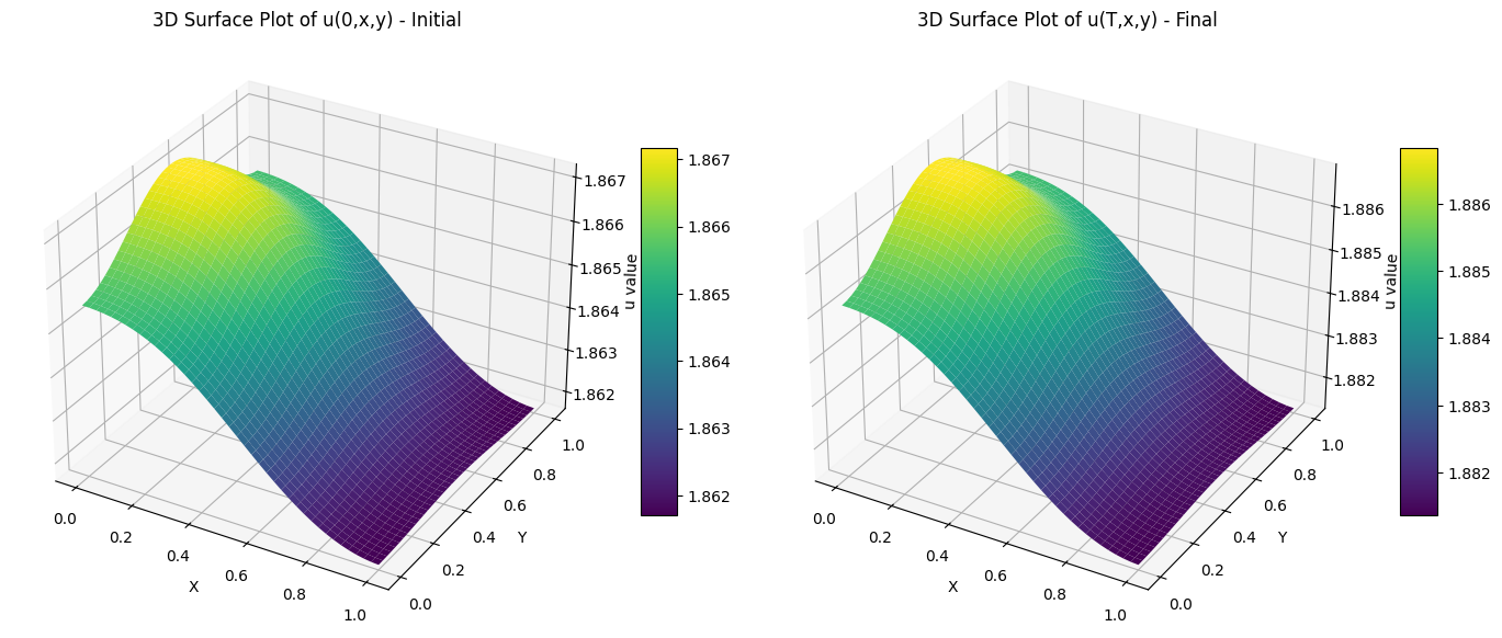
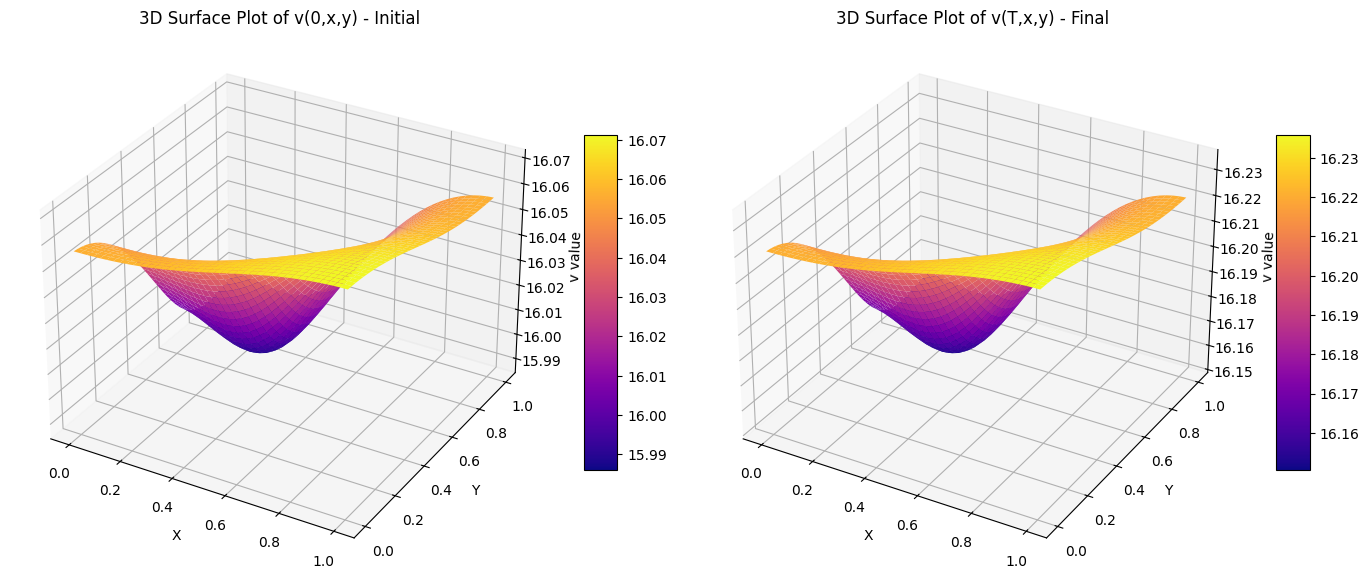
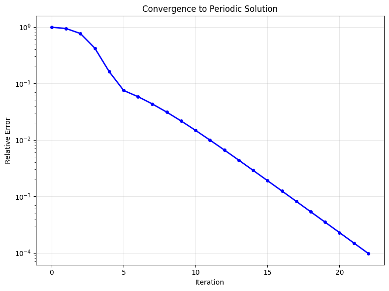
The numerical scheme successfully captures the periodic behavior predicted by the theoretical analysis. The IMEX approach provides a good balance between stability and computational efficiency, while the fixed-point iteration reliably converges to the periodic solution. The relaxation parameter \(\omega = 0.5\) was found to offer optimal convergence rates for the tested parameter regimes.
Future work could explore adaptive time-stepping strategies to further improve efficiency, as well as the extension of the method to handle more complex geometries and higher-dimensional problems.
Author Contributions: All authors contributed equally to the writing of this paper. All authors read and approved the final manuscript.
Conflicts of Interest: This work does not have any conflicts of interest.
Acknowledgments: The authors would like to express their sincere gratitude to the anonymous referee and the editor for their careful reading of the manuscript and their valuable comments, remarks, and suggestions that have greatly improved the quality of our paper.