
For decades, options trading and its theories have been studied, but more investigations almost had been remained almost up to the early 1970s. The Black-Scholes model (BSM) [1] indeed was accorded as some sort of victory for mathematical modeling in finance in a way that it has been relied on as an inherent tool in options trading as well as financial derivatives. As stated earlier in [2], the interest in pricing financial derivatives, including pricing choices is likely to be resulted from the fact that the minimization of losses develops out of fluctuations in prices regarding the underlying assets. The stock price which is a random variable evolving over time can assign the option price. The term random here, in the stochastic equation, must be considered as delta-correlated, that is to say the prices are calculated through white noise. We recall that a Brownian motion is in parallel with a process, whose increments are independent stationary normal random variables [3]. Since the stock price cannot be negative, Samuelson [4] offered the exploitation of this process for the illustration of the return of the stock price. This will lead to the stock price formation as a geometric (or exponential) Brownian motion. Javaheri states in [5] that constant volatility assumption does not manage to justify the being of the volatility smile besides the stock distribution leptokurtic character. The hazard rate tangent approximation was applied for the assessment of upper and lower bounds of the option price in case of parameters with time dependence in the Black-Scholes model by Roberts and Shortland [6]. Authors of [7] argued for a simple method to calculate estimates of barrier option prices with time dependent parameters accurately. These parameters are based upon simulation of the fixed barrier via small oscillating amplitude in a slowly fluctuating barrier. Company et al. [8] obtained an integral formula for a solution for Black-Scholes equation. This solution can be used to valuate the stock options with discrete dividend payments by utilization of Mellin transform. Authors of [9] discovered solutions for the inhomogeneous Black-Scholes equations with time dependent coefficients. They also studied min-max estimates, gradient estimates, monotonicity and convexity of the solutions with respect to the stock price variable. Farnoosh et al. [10] explored the problem of discrete double barrier option pricing considering the time dependent models. In these models, the parameters risk free rate, dividend and volatility have been deduced to be deterministic functions of time. They proposed a numerical method and calculated the Greeks of contract. Okelola et al. [11] solved the partial differential equation through the Lie group approach considering its association with the pricing of power options accompanied by time-dependent parameters. During the last two decades, the nonlinear Black-Scholes equation has gained popularity on account of the fact that it can offer more accurate values by means of taking the transaction costs as a workable assumption into consideration.
Barls and Soner [12] provided a model based on the assumption that an exponential utility function can characterize the investor’s preferences. After utilizing the exponential utility function, they proved the implementation of the theory of stochastic optimal control, when \(V\) is the unique viscosity solution of the Black-Scholes equation
with modified volatility function
and with the following non-differentiable terminal and time-dependent boundary conditions
where \(S\) is the price of the underlying asset, \(T\) is the maturity date, \(r\) is the risk-free interest rate, \(\sigma_0\) is the asset volatility, and \(a\) is transaction cost. Function \(\Psi(A)\) is the solution of the following nonlinear ordinary differential equation
There is no closed-form or analytical solution to this because of the coefficient \(x\) in the radical, but a good approximate solution can be obtained using numerical methods. In this work, first we present the solution of the Black-Scholes equation with constant parameters following [13], then we present a solution of the Black-Scholes equation with time-dependent volatility and time-dependent risk-free interest rate following [14]. Authors of [15] analyzed the obtained analytical solutions of a time-space-fractional Black-Scholes model utilizing a modified differential transform method. Jena et al [16] investigated the Ivancevic option pricing model which is an alternative of the standard Black-Scholes pricing equation with fractional reduced differential transform method to solve the Schrodinger type option pricing model. In [17–18], the solve and convergence of a fourth order finite difference method for the 2-D unsteady, viscous incompressible Boussinesq equations, based on the vorticity-stream function formulation have been investigated. Fathy et al. [19] investigated the Maxwell equations by a long-stencil fourth order finite difference method over a Yee grid. Authors of [20] analyzed an energy stable numerical scheme for the Cahn-Hilliard equation, with second order accuracy in time and the fourth order finite difference approximation in space. Lastly, we apply Saul’yev finite difference scheme to solve the fully nonlinear Black-Scholes equation. To the best of our knowledge this is the first time that the Saul’yev scheme is proposed to solve the Barles’ and Soner’s model in the Black-Scholes equation.
Among the vast spectrum of NPDEs, the nonlinear models have emerged as paradigmatic models for understanding nonlinear media [21–22]. The nonlinear equations have been extensively studied using multiple analytical approaches, including the cubic B-splines method [23], the Legendre approximation method [24], the Hirota’s bilinear operator [25], soliton and lump and travelling wave solutions [26], ranking extreme efficient decision method [27], and the multi-dimensional generalizations [28].
In the following, the content of other sections of the article are presented in brief. The solution of the Black-Scholes equation with constant parameters is presented in §2. The Black-Scholes equation with time-dependent parameters is transformed directly into a Black-Scholes equation with time-independent parameters in §3. The Saul’yev finite difference scheme is proposed for fully nonlinear Black-Scholes equation in §4. Finally, the conclusions are summarized in §5.
The Black-Scholes equation for a European call option with value \(u(S,t)\) is
which \(\sigma_c\) and \(r_c\) are constant. Its condition is in backward form, with final data given at \(t=T\)
which \(E\) is the strike price and boundary conditions
We follow [13] to put
This results in the equation
where \(k=\frac{2r_c}{\sigma_c ^2}\) and \(\nu(x,0)=\max(e^x-1,0)\). By setting
which \(\alpha\) and \(\beta\) should be found, one gets
By considering \(\beta=\alpha^2+(k-1)\alpha-k\) and \(2\alpha+(k-1)=0\), we will have an equation without \(U\) and \(\frac{\partial U}{\partial x}\). Therefore, \(\alpha\) and \(\beta\) are
Then
and
with
The solution of the diffusion Eq. (14) with initial condition (15) is
By change of variable \(-\frac{x-s}{\sqrt{2\tau}}=X\)
which
and
The cumulative distribution function for the normal distribution is
We consider
then
Variables of (8) can be written as
Therefore by (17), (22) and (23) we obtain the solution of (5) as
which
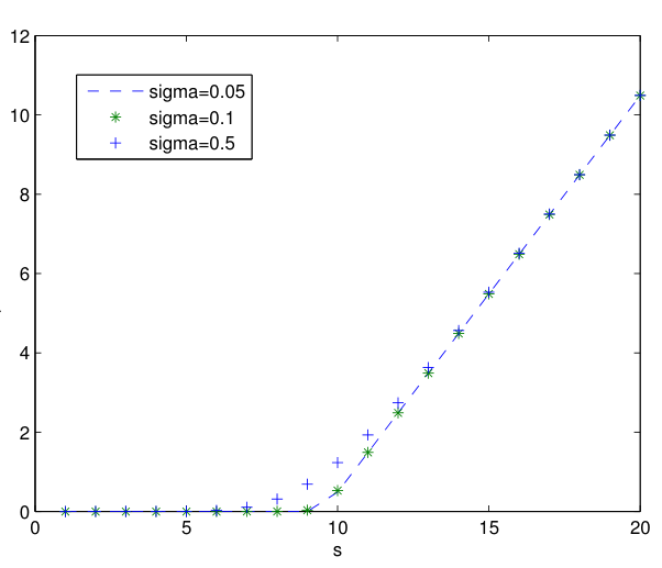
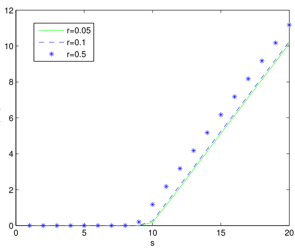
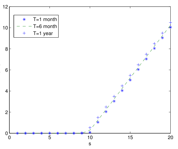
We compute the Black-Scholes price for several volatilities in \(t=0\). As we can see in Figure 1, the value of the call option increases as \(\sigma_0\) increases. Moreover, the Black-Scholes price is computed for several interest rates and maturity times. In Figures 2 and 3 we can see that the value of the call option increases as \(r\) and \(T\) increase.
In this section, we follow [14] to solve Black-Scholes equation with nonconstant volatility parameter as well as risk-free interest rate. Consider the equation:
with
We want to transform (26) and (27) into the Black-Scholes equation with constant parameters
with
The parameters \(\sigma_c\), \(r_c\) and \(\overline{E}\) are assumed to be positive. The transformation is such that \(\tau=\overline{T}\) when \(t=T\). Put
We should find \(h(t)\), \(\phi(t)\) and \(\psi(t)\). The chain rule gets \begin{align*} \frac{\partial V}{\partial t}=&h(t)\Big(\frac{\partial u}{\partial x}\phi'(t)S+\frac{\partial u}{\partial \tau}\psi'(t)\Big)+h'(t)u,\\ \frac{\partial V}{\partial S}=&h(t)\phi(t)\frac{\partial u}{\partial x},\\ \frac{\partial^2 V}{\partial S^2}=&h(t)\phi(t)^2\frac{\partial^2 u}{\partial x^2}. \end{align*}
By substituting into (26), one becomes \begin{align} h(t) &\Bigg( \frac{\partial u}{\partial x}\phi'(t)S + \frac{\partial u}{\partial \tau}\psi'(t)\Bigg)+h'(t)u+ \frac{\sigma^2(t)}{2}S^2h(t)\phi(t)^2\frac{\partial^2 u}{\partial x^2} +r(t)S h(t)\phi(t)\frac{\partial u}{\partial x}-r(t)h(t)u=0. \nonumber \end{align}
Rearranging terms gives \begin{align} \frac{\partial u}{\partial \tau} & + \frac{\sigma^2(t)\phi(t)^2S^2}{2\psi'(t)}\frac{\partial^2 u}{\partial x^2}+ \frac{r(t)\phi(t)S+\phi'(t)S}{\psi'(t)}\frac{\partial u}{\partial x} + \frac{h'(t)-r(t)h(t)}{h(t)\psi'(t)}u=0. \nonumber \end{align}
In comparison with (28), we see
From (31) and \(x=\phi(t) S\), we have \begin{equation*} \frac{\sigma^2(t)}{\sigma_c^2}=\psi'(t). \end{equation*}
By integrating
where \(C_1\) is an arbitrary constant of integration. From (32) we have as below \begin{equation*} \frac{\phi'(t)}{\phi(t)}=r_c\psi'(t)-r(t). \end{equation*}
So
From (33) we have \begin{equation*} \frac{h'(t)}{h(t)}=r(t)-r_c\psi'(t). \end{equation*}
Therefore
Constants of integration \(C_1\), \(C_2\) and \(C_3\) can be obtained by \begin{equation*} \max(S-E,0)=V(S,T)=h(T)u(x,\overline{T})=h(T)\max(x-\overline{E},0). \end{equation*}
On the other hand, we see \begin{equation*} h(T)\max(x-\overline{E},0)=h(T)\max(\phi(T)S-\overline{E},0)=h(T)\phi(T)\max\left( S-\frac{\overline{E}}{\phi(T)} ,0\right). \end{equation*}
Therefore, we must have
and
Also from (37) and (36) we have
Lastly, from \(\psi(\overline{T})=\overline{T}\) and (34), we get
We shall, therefore, obtain the solution of (26) as
\begin{equation*} x=\frac{\overline{E}}{E}exp\Bigg(-\int_t^T\Big(\frac{r_c}{\sigma_c^2}\sigma(z)-r(z)\Big)dz\Bigg)S, \end{equation*} \begin{equation*} \tau=-\frac{1}{\sigma_c^2}\int_{t}^{T}\sigma_u^{2}du+\overline{T}, \end{equation*} which as said in the previous section \(u(x,\tau)\) in (42) is as below form \begin{equation*} u(x,\tau)=xN(d_1)-\overline{K}e^{-r_c(\overline{T}-\tau)}N(d_2), \end{equation*} \begin{equation*} d_1=\frac{\ln(\frac{x}{\overline{K}})+(r_c+\frac{\sigma_c^2}{2})(\overline{T}-\tau)}{\sigma_c\sqrt{\overline{T}-\tau}}, d_2=\frac{\ln(\frac{x}{\overline{K}})+(r_c-\frac{\sigma_c^2}{2})(\overline{T}-\tau)}{\sigma_c\sqrt{\overline{T}-\tau}}. \end{equation*}
In this section we consider the Barles’ and Soner’s model for nonlinear Black-Scholes Eqs. (1)-(3). Nonlinear nature of this model has necessitated using a numerical method to price the option. In order to ease the numerical solution of nonlinear Eqs. (1)-(3) for the European call option, we transform the problem into a forward parabolic problem. Using the following variable transformations
Black-Scholes Eq. (1) yields
{where \(r\) is the risk-free interest rate, \(\sigma_0\) is the asset volatility, and \(a\) is transaction cost} and conditions (3) were transformed into
So that \(u(B,\tau) = B\) or a linear extrapolation consistent with \(u \sim x\). We use Saul’yev finite difference scheme which not only is explicit, but also is unconditionally stable. Conditions need to be created \(1+\Psi(a^2x^2u_{xx}\geq0\). The scheme is monotone and consistent and then it converges to the unique viscosity solution of the problem {(44) where is defined in a finite domain \([0,\infty)\times [0,T]\). Take the domain \([0,B]\times [0,T]\) and a grid of mesh points \((x,\tau)=(x_i,\tau_n)\), which \(x_i=ih\), \(i=0,1,\cdots,M\) and \(\tau_n=nk\), \(n=0,1,\cdots,N\). The spatial step size is \(h=\frac{B}{M}\) and the time step size is \(k=\frac{T}{N}\). Denote approximation of \(u(x_i,\tau_n)\) by \(u_i^n\) and define the finite difference approximations of derivatives
From (44) we have the finite difference scheme as follows
If we consider \(\alpha_i^n\) instead of \(\Delta_i^n\) in \(\big(1+\Psi(a^2x_i^2\Delta_i^n)\big)\) in (49), the scheme can only be solved by a nonlinear iteration in each time step which is quite time-consuming. By denoting \(\frac{\sigma^2}{2}\big(1+\Psi(a^2x_i^2\triangle_i^n)\big)x_i^2=\alpha_i^n\) and \(s=\frac{k}{h^2}\), we have \begin{equation*} \frac{u_i^{n+1}-u_i^n}{k}-\alpha_i^n\left(\frac{u_{i+1}^{n}-u_i^{n}-u_i^{n+1}+u_{i-1}^{n+1}}{h^2}\right)=0, \end{equation*} or \begin{equation*} \frac{u_i^{n+1}-u_i^n}{s}-\alpha_i^n\left(u_{i+1}^{n}-u_i^{n}-u_i^{n+1}+u_{i-1}^{n+1}\right)=0, \end{equation*}
We can rewrite (50) as
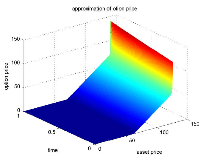
with the calculations proceeding in the direction of increasing x, (from left to right). The scheme can be written in matrix form \(A^nu^{n+1}=B^nu^{n}\). Matrixes \(A^n\) and \(B^n\) are tridiagonal \begin{equation*} \mathbf{A}^n = \left( \begin{array}{ccccccc} 1+s\alpha_0^n & 0 & 0 & 0 & 0 &… & 0\\ – s\alpha_1^n & 1+s\alpha_1^n & 0 & 0 & 0 & … & 0 \\ 0 & – s\alpha_2^n & 1+s\alpha_2^n & 0 & 0 & … & 0 \\ 0 & 0 & – s\alpha_3^n & 1+s\alpha_3^n & 0 & … & 0 \\ \vdots & \vdots & \vdots & \vdots & \vdots &\ddots & \vdots\\ 0 & 0 & 0 & 0 & 0 & – s\alpha_M^n & 1+s\alpha_M^n \end{array} \right), \end{equation*} and \begin{equation*} \mathbf{B}^n = \left( \begin{array}{ccccccc} 1-s\alpha_0^n & s\alpha_0^n & 0 & 0 & 0 &… & 0\\ 0 & 1-s\alpha_1^n & s\alpha_1^n & 0 & 0 & … & 0 \\ 0 & 0 & 1-s\alpha_2^n & s\alpha_2^n & 0 & … & 0 \\ \vdots & \vdots & \vdots & \vdots & \vdots &\ddots & \vdots\\ 0 & 0 &0 & 0 & 0 & 1-s\alpha_{M-1}^n & s\alpha_{M-1}^n \\ 0 & 0 & 0 & 0 & 0 & 0 & 1-s\alpha_M^n \end{array} \right), \end{equation*} we utilize a \(1.80\) GHz Intel(R) Core(TM) \(i5-3337 U\) with \(4\) GB memory for our calculations. The technique was employed in MATLAB R2013a. Transaction costs \(a=0.02, 0.015, 0.01, 0.005\) and\(0\) are chosen from [12]. The compared methods in the following Table are the implicit Crank Nicolson (CN) scheme and Backward Time, Centered Space (BTCS) where is an implicit finite difference method used to numerically solve the Black-Scholes partial differential equation (PDE) for option pricing. By discretizing time and stock price, BTCS offers unconditional stability, making it more robust than explicit methods (FTCS) for large volatility or long time steps. Results are shown in Table 1 by \(M=20\), \(N=10\) and the linear case (\(a=0\)) is plotted in Figure 4.
| transaction cost | \(e_{max}(BTCS)\) | \(e_{max}(CN)\) |
|---|---|---|
| \(0.02\) | \(1.027e-1\) | \(5.20e-2\) |
| \(0.015\) | \(8.860e-2\) | \(4.48e-2\) |
| \(0.01\) | \(7.850e-2\) | \(3.96e-2\) |
| \(0.005\) | \(7.230e-2\) | \(3.65e-2\) |
| \(0\)(Linear) | \(7.030e-2\) | \(3.54e-2\) |
Now, we prove consistency, monotonicity and stability.
Theorem 1 (Consistency). Consider Eq. (44) with exact solution \(u\) as \(L(u)=0\), and let \(F(u_i^n)=0\)represent the finite difference scheme (49). Hence \begin{eqnarray} T_i^n(u)&=&F(u_i^n)-L(u_i^n) \nonumber\\ &=&\frac{u_i^{n+1}-u_i^n}{k}-\frac{\sigma_0^2}{2}\big(1+\Psi(a^2x_i^2\triangle_i^n)\big)x_i^2\delta_i^n -\Big(u_{\tau}-\frac{\sigma_0^2}{2}\big(1+\Psi(a^2x^2u_{xx})\big)x^2u_{xx}\Big)_i^n. \nonumber \end{eqnarray} with
and
and also
Then, we get
and
Therefore, the problem of consistency is the problem of finding the condition for which a discrete problem is an approximation of the corresponding continuous problem.
Theorem 2 (Monotonicity). If the time step in the numerical scheme (51) is selected such that
then the scheme is monotone.
Proof. See [29].
The unconditional stability only holds under additional constraints (e.g., bounds on \(\alpha_i^n\)), state them explicitly.
Theorem 3 (Stability). Considering \(u(exact)_i^n-u(app)_i^n=e_i^n\), and the following
Let \(1+\Psi>0\), and hence \(\alpha_i^n>0\), for all \(n\) and \(i\), on the other hand, because \(s>0\), hence we have
and
Therefore, the spectral radius \(\rho(M)=\max\Big\{\left\vert\frac{1-s\alpha_i^n}{1+s\alpha_i^n}\right\vert, i=0,\ldots M. \Big\}<1\), and the Saul’yev finite difference scheme is unconditionally stable.
We appraised the Black-Scholes equation solution with constant parameters in this article. Then, the Black-Scholes equation with time-dependent parameters was transformed directly into a Black-Scholes equation with time-independent parameters. In the real financial market, the volatility was more complicated which leads to the fully nonlinear Black-Scholes equation. Because this equation does not have an exact solution, we solved this nonlinear partial differential equation numerically. The Saul’yev scheme was applied to solve the Barles’s and Soner’s model of fully nonlinear Black-Scholes equation which was unconditionally stable and explicit and converges to the unique viscosity solution.