
1. Introduction
This technical paper addresses the minimum dominating set problem and aims to determine the minimum dominating set of a graph, complementing and extending the results of [1]. A dominating set of a graph \(G\) is a set \(S\) of vertices of \(G\) such that every vertex \(v\) of \(G\) is either in \(S\) or adjacent to a vertex of \(S\). A minimum dominating set is a dominating set of minimum size.
The minimum dominating set problem for cubic graphs is known to be NP-complete [2], which implies that the problem is NP-complete for general graphs as well. In this work, we extend the order-decreasing sequence used in the proof of the theorem in [1], thereby generalizing the result from graphs of maximum degree 3 to arbitrary graphs.
As a main part, this paper introduces three polynomial-time algorithms for graphs and provides technical refinements, ultimately leading that the problem lies in P, thus establishing that P = NP.
2. Notation
In this paper, a graph \(G\) is finite, undirected, and simple with the vertex set \(V\) and edge set \(E\). We follow the notations presented in [3]. For a vertex \(v \in V(G)\), the open neighborhood, denoted by \(N_G(v)\), is \(\{ u \in V(G) \colon uv \in E(G) \}\), and the closed neighborhood, denoted by \(N_G[v]\), is \(N_G(v) \cup \{v\}\), also for a set \(W \subseteq V(G)\), let \(N_G(W) = \bigcup_{v \in W} N_G(v)\) and \(N_G[W] = N_G(W) \cup W\). A dominating set \(X \subseteq V(G)\) is such that \(N_G[X] = V(G)\). A minimum dominating set, called a d-set, is a dominating set of minimum size. \(X\)-3-path is a path or cycle of length at least 2 with labels for every 3 vertices, or a path of length 1 with a label on at most one of two vertices. Two cycles \(C_1\) and \(C_2\) are said to be connecting without seams if \(X\)-3-path can be assigned to \(C_1\) and \(C_2\) respectively so that \(C_1 \cap C_2\) is one \(X\)-3-path.
3. Algorithms and complements
We consider a connected graph \(G\), otherwise consider each component one by one. First, we introduce the algorithm Scheme \(\mathbf{K}\), Algorithm 1 and 2.
In the algorithm Scheme \(\mathbf{K}\), if there are multiple ways to label vertices during the labeling process, we take the procedure for labeling (\(*0\)): Let \(U_0\) be the set of all unlabeled vertices not adjacent to the labeled vertices in \(G_k\). For the two adjacent vertices \(y_1\) and \(y_2\), select \(y_1\) if \(N_{G_k}[y_2] \cap U_0 \subsetneq N_{G_k}[y_1]\), select \(y_2\) if \(N_{G_k}[y_1] \cap U_0 \subsetneq N_{G_k}[y_2]\), select \(y_1\) if \(y_1\) is a cut vertex of \(G\) and \(y_2\) is not a cut vertex of \(G\), select \(y_2\) if \(y_2\) is a cut vertex of \(G\) and \(y_1\) is not a cut vertex of \(G\), select the first taken vertex \(y_1\) or \(y_2\) otherwise.
Proposition 1 ([3]). A graph is 2-connected if and only if it can be constructed from a cycle by successively adding \(H\)-paths to graphs \(H\) already constructed.
Algorithm 1: Scheme \(\mathbf{K}\): construction applied to a connected graph \(G\) – Part 1
Input: A connected graph \(G\)
Output: A resulting graph \(\mathbf{K}(G)\) and a tree \(T(G)\)
| 1 | if \(|V(G)| \leq 2\) then |
| 2 | \(T \leftarrow \varnothing\); |
| 3 | assign a label to some \(v \in V(G)\); |
| 4 | add a vertex to \(T\); |
| 5 | return \(G\) as \(\mathbf{K}(G)\) and \(T\) as \(T(G)\); |
| 6 | \(G_0 \leftarrow G\) and \(k \leftarrow 0\); |
| 7 | \(T_0 \leftarrow \varnothing\) and \(l \leftarrow 0\); |
| 8 | repeat |
| 9 | Let \(x\) be a cut vertex of \(G_k\). |
| 10 | foreach pairs of distinct components \(C_1\), \(C_2\) of \(G_k – x\) do |
| 11 | foreach pairs of vertices \(u \in V(C_1) \cap N_{G_k}(x)\), \(v \in V(C_2) \cap N_{G_k}(x)\) do |
| 12 | add an edge \(uv\) to \(G_k\); |
| 13 | \(k \leftarrow k + 1\); |
| 14 | until there exists a cut vertex in \(G_k\) |
| 15 | Find any induced cycle \(C\) in \(G_k\). |
| 16 | if length of \(C\) is 0 mod 3 then |
| 17 | assign \(X\)-3-path to \(C\) in \(G_k\), following the procedure for labeling (\(*0\)); |
| 18 | add \(C\) as a root vertex to \(T_l\); |
| 19 | \(l \leftarrow l + 1\); |
| 20 | else if length of \(C\) is 2 mod 3 then |
| 21 | take any 4-path \(x_1x_2x_3x_4 \subseteq C\); |
| 22 | add edges \(x_1x_3\), \(x_2x_4\), \(x_1x_4\) to \(G_k\); |
| 23 | \(k \leftarrow k + 1\); |
| 24 | assign \(X\)-3-paths to 0 mod 3 induced cycles connecting without seams in the formed subgraph (call this subgraph (a)), following the procedure for labeling (\(*0\)); |
| 25 | add each 0 mod 3 induced cycle as a vertex (set one of them as a root vertex) and one of its connections with the 0 mod 3 induced cycles in the subgraph (a) as an edge to \(T_l\); |
| 26 | \(l \leftarrow l + 1\); |
| 27 | else |
| 28 | take any 4-path \(x_1x_2x_3x_4 \subseteq C\); |
| 29 | add edges \(x_1x_3\) and \(x_2x_4\) to \(G_k\); |
| 30 | \(k \leftarrow k + 1\); |
| 31 | assign \(X\)-3-paths to 0 mod 3 induced cycles connecting without seams in the formed subgraph (call this subgraph (b)), following the procedure for labeling (\(*0\)); |
| 32 | add each 0 mod 3 induced cycle as a vertex (set one of them as a root vertex) and one of its connections with the 0 mod 3 induced cycles in the subgraph (b) as an edge to \(T_l\); |
| 33 | \(l \leftarrow l + 1\); |
| 34 | Find any shortest path \(P\) over all two vertices \(v_1\) and \(v_2\) lying on previously assigned \(X\)-3-path in \(G_k\) such that \(X\)-3-path has not been assigned to \(\mathring{v}_1P\mathring{v}_2\) yet. |
Algorithm 2: Scheme \(\mathbf{K}\) – Part 2
| 1 | if such a path \(P\) exists then |
| 2 | Let \(P’\) be the previously assigned \(X\)-3-path of length at least 2 containing \(v_1\) and \(v_2\). |
| 3 | if \(v_1Pv_2P’v_1\) forms a cycle of length 0 mod 3 in \(G_k\) then |
| 4 | assign \(X\)-3-path to \(v_1Pv_2P’v_1\) in \(G_k\) while maintaining or deleting the labels of existing \(X\)-3-path; |
| 5 | add \(v_1Pv_2P’v_1\) as a vertex and one of its connections with the 0 mod 3 cycles which have a part of \(v_1P’v_2\) and contained as the vertices in \(T_l\) already as an edge to \(T_l\); |
| 6 | \(l \leftarrow l + 1\); |
| 7 | else if \(v_1Pv_2P’v_1\) forms a cycle of length 2 mod 3 in \(G_k\) then |
| 8 | take any 4-path in \(v_1Pv_2P’v_1\) and add three edges to \(G_k\) as in subgraph (a); |
| 9 | \(k \leftarrow k + 1\); |
| 10 | if possible then |
| 11 | assign \(X\)-3-paths to 0 mod 3 induced cycles connecting without seams in the subgraph (a) while maintaining or deleting the labels of existing \(X\)-3-path, following the procedure for labeling (\(*0\)); |
| 12 | else |
| 13 | \(k \leftarrow k – 1\) and goto step 8; |
| 14 | add each 0 mod 3 induced cycle as a vertex and one of its connections with the 0 mod 3 induced cycles in the subgraph (a) (or one of its connections with the 0 mod 3 cycles which have a part of \(v_1P’v_2\) and contained as the vertices in \(T_l\) already) as an edge to \(T_l\); |
| 15 | \(l \leftarrow l + 1\); |
| 16 | else if \(v_1Pv_2P’v_1\) forms a cycle of length 1 mod 3 in \(G_k\) then |
| 17 | take any 4-path in \(v_1Pv_2P’v_1\) and add two edges to \(G_k\) as in subgraph (b); |
| 18 | \(k \leftarrow k + 1\); |
| 19 | if possible then |
| 20 | assign \(X\)-3-paths to 0 mod 3 induced cycles connecting without seams in the subgraph (b) while maintaining or deleting the labels of existing \(X\)-3-path, following the procedure for labeling (\(*0\)); |
| 21 | else |
| 22 | \(k \leftarrow k – 1\) and goto step 17; |
| 23 | add each 0 mod 3 induced cycle as a vertex and one of its connections with the 0 mod 3 induced cycles in the subgraph (b) (or one of its connections with the 0 mod 3 cycles which have a part of \(v_1P’v_2\) and contained as the vertices in \(T_l\) already) as an edge to \(T_l\); |
| 24 | \(l \leftarrow l + 1\); |
| 25 | goto step 34 of Part 1 (continue the loop); |
| 26 | else |
| 27 | break the loop; |
| 28 | return \(G_k\) as \(\mathbf{K}(G)\) and \(T_l\) as \(T(G)\); |
Fact 1. In a 2-connected graph, any two vertices are connected by a path along edges in some ear of its ear decomposition.
Proof. The statement is proved by induction on ears. As a base case, if \(v\) and \(w\) in first ear (cycle), path exists trivially. Assume path exists for first \(k\) ears, add \((k+1)\)-th ear if needed. 2-connectedness ensures every vertex is in some ear. We can concatenate paths along endpoints of ears. \(\square\)
Proposition 2. In the algorithm Scheme \(\mathbf{K}\) – Part 1 step 34, it is possible to find previously assigned \(X\)-3-path between \(v_1\) and \(v_2\).
Proof. In Fact 1, by replacing each ear with \(X\)-3-path, we have the statement. \(\square\)
Proposition 3. In the algorithm Scheme \(\mathbf{K}\) – Part 1 step 34, a cycle is created by choosing the shortest path connecting the two endpoints of \(X\)-3-path. If the length of the cycle is 1 mod 3 or 2 mod 3, choose any 4-path and add edges according to the rule. In the algorithm Scheme \(\mathbf{K}\) – Part 2 step 11 and 20, for some 4-path in the cycle, \(X\)-3-paths can be assigned to 0 mod 3 induced cycles connecting without seams in the subgraph while maintaining or deleting the labels of existing \(X\)-3-paths, following the procedure for labeling (\(*0\)).
Proof. Given the length of the existing \(X\)-3-path \(X\) (0, 1, 2 mod 3), the labeling method \(Y\) (3 rotation), the length of the cycle \(Z\) (1, 2 mod 3), and the 4-path selection method \(A\) (\(\mathcal{O}(n)\) for \(n = |V(G)|\)), we obtain the proposition by analyzing all cases of \(X \times Y \times Z \times A\). \(\square\)
Note that \(\mathbf{K}(G)\) and \(T(G)\) are not unique and constructed from \(G\) arbitrarily. By the scheme, \(\mathbf{K}(G)\) is 2-connected with \(V(G) = V(\mathbf{K}(G))\) and \(E(G) \subseteq E(\mathbf{K}(G))\), and all edges in \(\mathbf{K}(G)\) are covered by at least one set of \(X\)-3-paths but may be covered by other set of \(X\)-3-paths with the rotation of labels. We have a tree-structured list \(T(G)\) of 0 mod 3 cycles connecting without seams. The label rotation follows this list. Choose an initial vertex to label from a cycle contained as the root vertex of \(T(G)\), and assign \(X\)-3-paths to the cycles in the list.
Consider labeling vertices by assigning \(X\)-3-paths to the cycles of length 0 mod 3 connecting without seams in \(\mathbf{K}(G)\) following \(T(G)\). (Note that certain cycles may not be counted for the labeling, and have as few labeled vertices as possible.) After selecting the first vertices to label, if there are multiple ways to label vertices during the labeling process, those vertices are two adjacent degree 3 vertices in \(K^4 – e \subseteq \mathbf{K}(G)\) for some \(e \in E(K^4)\) (call the two vertices alternative vertices). Now, we take the procedure for labeling (\(*1\)): Let \(U_0\) be the set of all unlabeled vertices not adjacent to the labeled vertices in \(\mathbf{K}(G)\). For the alternative vertices \(y_1\) and \(y_2\), select \(y_1\) if \(N_{\mathbf{K}(G)}[y_2] \cap U_0 \subsetneq N_{\mathbf{K}(G)}[y_1]\), select \(y_2\) if \(N_{\mathbf{K}(G)}[y_1] \cap U_0 \subsetneq N_{\mathbf{K}(G)}[y_2]\), select \(y_1\) if \(y_1\) is a cut vertex of \(G\) and \(y_2\) is not a cut vertex of \(G\), select \(y_2\) if \(y_2\) is a cut vertex of \(G\) and \(y_1\) is not a cut vertex of \(G\), select the first taken vertex \(y_1\) or \(y_2\) otherwise.
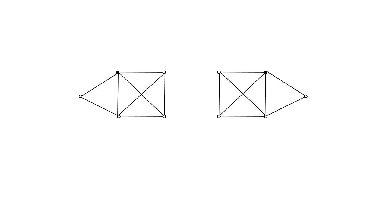
Remark 1 ([1]). Let \(X\) be a dominating set of \(G\). Every subset \(D \subseteq X\) is a d-set of \(G[N_G[D]]\) if and only if \(X\) is a d-set of \(G\).
Proposition 4. (i) For every labeling, the set of all labeled vertices is a minimal dominating set of \(\mathbf{K}(G)\). In addition, by selecting the first vertices to label following \(T(G)\) from the root vertex, the remaining labeled vertices is uniquely determined. (ii) For at least one labeling, the set of all labeled vertices is a d-set of \(\mathbf{K}(G)\).
Proof. Since every edge in \(\mathbf{K}(G)\) is covered by \(X\)-3-path, for every labeling, the set of all labeled vertices is an independent dominating set of \(\mathbf{K}(G)\), that is, a minimal dominating set of \(\mathbf{K}(G)\). After selecting the first vertices to label, if there are multiple ways to label vertices during the labeling process, we take the procedure for labeling (\(*1\)). Then the remaining labeled vertices are determined following \(T(G)\) uniquely. Therefore, the statement (i) holds. By Remark 1, the statement (ii) obviously holds. \(\square\)
Let \(Y\) be a d-set of \(\mathbf{K}(G)\) that is obtained by labeling. Let \(\mathcal{Y}\) be the set of all \(Y\). Regarding the handling of cut vertices of \(G\), the procedure for labeling (\(*1\)) is justified by Fact 2.
Fact 2. Suppose \(G\) has a cut vertex \(v\) and \(w \in N_G(v)\) is not a cut vertex. For \(Y_1, Y_2 \in \mathcal{Y}\) such that \(Y_1 \cap Y_2 \ne \emptyset\), if \(v \in Y_1 \setminus Y_2\) and \(w \in Y_2 \setminus Y_1\), then \(Y_1\) is better for a d-set of \(G\).
Proof. In the 0 mod 3 induced cycles constructed from \(v\) by the edge addition rules of the algorithm Scheme \(\mathbf{K}\) – Part 1 step 8, \(w\) does not dominate any other neighbor of \(v\) in \(G\), in contrast, \(v\) dominates all its neighbors in \(G\). \(\square\)
Definition 1. For \(\mathcal{Y}’ \subseteq \mathcal{Y}\), define \(\equiv\) so that two sets \(A_1, A_2 \in \mathcal{Y}’\) are equivalent if and only if every pair of sets in \(\mathcal{Y}’\) has nonempty intersection that is an initial vertex to label following \(T(G)\) from the root vertex.
Proposition 5. Let \(X\) be a d-set of \(G\). Let \(\mathcal{X}\) be the set of all \(X\). For some \(\mathcal{B} \in \mathcal{Y}/\equiv\) and for each \(Y \in \mathcal{B}\), there exists \(X \in \mathcal{X}\) such that \(Y = X\), otherwise, for each \(Y \in \mathcal{Y}\), there exists \(X \in \mathcal{X}\) such that \(Y \subseteq X\).
Proof. Let \(\mathcal{B} \in \mathcal{Y}/\equiv\). Consider labeling vertices in \(\mathbf{K}(G)\). For any \(Y_1, Y_2 \in \mathcal{B}\) such that \(Y_1 \ne Y_2\), the vertices of \(Y_1 \setminus Y_2\) and \(Y_2 \setminus Y_1\) are interchangeable and equivalent. By the definition of \(\mathbf{K}(G)\) and \(\mathcal{B}\), it suffices that considering subgraph (a) or (b) of \(\mathbf{K}(G)\). Now, \(N_{\mathbf{K}(G)}[Y_1 \setminus Y_2] = N_{\mathbf{K}(G)}[Y_2 \setminus Y_1]\). If \(Y_1\) is a dominating set of \(G\), then for some \(X \in \mathcal{X}\), \(X = Y_1\). Now, \(N_G[Y_2 \setminus Y_1] \setminus N_G[Y_1 \setminus Y_2] \subseteq N_G[Y_1] = V(G)\). By considering alternative vertices of the subgraph (a), we have \(N_G[Y_1 \setminus Y_2] \setminus N_G[Y_2 \setminus Y_1] \subseteq N_G[Y_2]\). Hence, \(N_G[Y_1] = N_G[Y_2]\). Suppose that for all \(Y \in \mathcal{Y}\), \(Y\) is not a dominating set of \(G\). Now, each \(Y_1\) and \(Y_2\) is not a dominating set of \(G\). By considering alternative vertices of the subgraph (b), we have \(N_G[Y_2 \setminus Y_1] \setminus N_G[Y_1 \setminus Y_2] \not\subseteq N_G[Y_1]\) and \(N_G[Y_1 \setminus Y_2] \setminus N_G[Y_2 \setminus Y_1] \not\subseteq N_G[Y_2]\). Hence, \(N_G[Y_1] \setminus N_G[Y_2] \ne \emptyset\) and \(N_G[Y_2] \setminus N_G[Y_1] \ne \emptyset\). Let \(\mathcal{B}_1, \mathcal{B}_2 \in \mathcal{Y}/\equiv\) with \(\mathcal{B}_1 \ne \mathcal{B}_2\). For any \(Y_3 \in \mathcal{B}_1\) and any \(Y_4 \in \mathcal{B}_2\), since \(Y_3 \cap Y_4 = \emptyset\) and each \(Y_3\) and \(Y_4\) is not a dominating set of \(G\), by considering not alternative vertices of the subgraph (a) or (b), it follows that \(N_G[Y_3] \setminus N_G[Y_4] \ne \emptyset\) and \(N_G[Y_4] \setminus N_G[Y_3] \ne \emptyset\). Now, \(Y\) is a d-set of \(G[N_G[Y]]\). Let \(W\) be a subset of \(V(G) \setminus Y\) with minimum size such that \(Y \cup W\) is a dominating set of \(G\). By Remark 1, \(Y \cup W\) is a d-set of \(G\). Indeed, \(\mathbf{K}(G)\) is covered by 0 mod 3 cycles connecting without seams, which have no assignments of less labeled vertices to be a d-set of \(\mathbf{K}(G)\). That is to say, \(\mathbf{K}(G)\) has no backtracking of the labeled vertices of \(Y\) by adding the vertices of \(W\). \(\square\)
Proposition 6. \(|\mathcal{Y}/\equiv| \leq |V(G)|\). \(Y \in \mathcal{B} \in \mathcal{Y}/\equiv\) contained as the subset of a d-set of \(G\) is determined in polynomial time.
Proof. Since each step in the algorithm Scheme \(\mathbf{K}\) is in polynomial time, by adding the all steps, \(\mathbf{K}(G)\) and \(T(G)\) are constructed from \(G\) in polynomial time. For each \(v \in V(G)\) to label initially, the equivalence class \(\mathcal{B} \in \mathcal{Y}/\equiv\) is defined as the label sets \(B(v)\), hence \(|\mathcal{Y}/\equiv| \leq |V(G)|\). By Proposition 4 and the definition of \(\mathcal{Y}\), \(B(v)\) is determined in polynomial time. By Proposition 5, \(B(v)\) contained as the subset of a d-set of \(G\) is determined in polynomial time. \(\square\)
Second, we introduce the algorithm Labeling-and-Prune procedure (Algorithm 3). It returns a label set \(L(G)\) of \(G\), which is \(Y \in \mathcal{B} \in \mathcal{Y}/\equiv\) contained as the subset of a d-set of \(G\).
Proposition 7. Let \(\mathcal{S}(G)\) be the set of all pairs \((\mathbf{K}(G), T(G))\) obtained from the algorithm Scheme \(\mathbf{K}\), \(\mathcal{L}(G)\) be the set of all \(L(G)\) obtained from the algorithm Labeling-and-Prune procedure, \(\mathcal{L}_0(G)\) be the set of all \(\mathcal{L}(G)\), and \(\mathcal{X}\) be the set of all d-sets of \(G\). Then, \(l : \mathcal{S}(G) \to \mathcal{L}_0(G)\) can be defined as for all \(S \in \mathcal{S}(G)\), \(l(S)\) satisfies for all \(L(G) \in l(S)\) and for some \(X \in \mathcal{X}\), \(L(G) \subseteq X\).
Proof. It is straightforward from Proposition 5. \(\square\)
Third, we introduce the algorithm extendWithProp8 (Algorithm 4) as follows. For a graph \(F\), it returns a minimum dominating set of \(F\), which is written by \(X(F)\).
Proposition 8 ([1]). Let \(Y = L(G)\). Let \(G’\) be a graph obtained by deleting \(Y\) from, and adding edges to all vertex pairs of \(\bigcup_{y \in Y}N_G(y)\) to \(G\). Let \(Z_1\) be a d-set of \(G’\). Let \(G” = G – N_G[Y]\) and \(Z_2\) be a d-set of \(G”\). If \(|Z_1| \lt |Z_2|\), then \(Y \cup Z_1\) is a d-set of \(G\), and \(Z_1 \cap \bigcup_{y \in Y}N_G(y) \ne \emptyset\). If \(|Z_1| \geq |Z_2|\), then \(Y \cup Z_2\) is a d-set of \(G\).
Theorem 1. The d-set of a graph is determined in polynomial time.
Proof. It follows the algorithm extendWithProp8. The computation of \(L(G)\) for a component \(G\) of the graph \(F\) is in polynomial time by Proposition 6. The remaining vertices of a d-set of \(F\) from \(\bigcup L(G)\) are derived from Proposition 8 with the recursion of extendWithProp8 for \(G’\) and \(G”\), which have the order-decreasing sequence. The number of recursions in extendWithProp8 is \(\mathcal{O}(n^2)\) for \(n = |V(G)|\) by multiplying the height \(n\) and the width \(n\). Hence, by adding each polynomial step, all computations in extendWithProp8 can be performed in polynomial time. \(\square\)
Algorithm 3: Labeling-and-Prune procedure: labeling method on \(\mathbf{K}(G)\)
Input: A connected graph \(G\), \(\mathbf{K}(G)\), \(T(G)\)
Output: A label set \(L(G)\)
| 1 | if \(|V(G)| \leq 2\) then |
| 2 | \(L \leftarrow \varnothing\); |
| 3 | add a vertex in \(V(G)\) to \(L\); |
| 4 | return \(L\) as \(L(G)\); |
| 5 | \(\mathcal{L} \leftarrow \varnothing\); |
| 6 | foreach \(v \in V(G)\) in a cycle of \(\mathbf{K}(G)\) contained as the root vertex of \(T(G)\) do |
| 7 | label \(v\); |
| 8 | create a temporary labelling \(L\); |
| 9 | assign \(X\)-3-path to a cycle of \(\mathbf{K}(G)\) contained as the root vertex of \(T(G)\) and add labels to \(L\); |
| 10 | foreach 0 mod 3 cycle \(D\) of \(\mathbf{K}(G)\) contained as the adjacent vertex in \(T(G)\) do |
| 11 | assign \(X\)-3-path to \(D\) while maintaining or deleting the labels of existing \(X\)-3-path, following the procedure for labeling (\(*1\)); |
| 12 | add labels to \(L\); |
| 13 | add \(L\) to \(\mathcal{L}\) and record its size \(|L|\); |
| 14 | \(\mathcal{Y} \leftarrow \{Y \in \mathcal{L} \colon |Y| \text{ is minimum}\}\); |
| 15 | foreach \(Y \in \mathcal{Y}\) do |
| 16 | if \(Y\) is a dominating set of \(G\) then |
| 17 | return \(Y\) as \(L(G)\); |
| 18 | choose any \(Y \in \mathcal{Y}\) and return \(Y\) as \(L(G)\); |
Algorithm 4: extendWithProp8: determination of the remaining vertices for a d-set
Input: A graph \(F\), \(L(G)\) for a component \(G\) of \(F\)
Output: A minimum dominating set \(X(F)\)
| 1 | if \(F = \varnothing\) then |
| 2 | return \(\varnothing\) as \(X(F)\); |
| 3 | \(W \leftarrow \varnothing\); |
| 4 | foreach component \(G\) of \(F\) do |
| 5 | \(S \leftarrow L(G)\); |
| 6 | if \(V(G) \setminus N_G[S] = \varnothing\) then |
| 7 | \(W \leftarrow W \cup S\); |
| 8 | goto step 4; |
| 9 | Let \(G’\) be constructed by deleting \(S\), and for every pair \(w_1, w_2 \in \bigcup_{s \in S}N_G(s)\), adding an edge \(w_1w_2\) to \(G\). |
| 10 | \(Z_1 \leftarrow \mathrm{extendWithProp}8(G’)\); |
| 11 | \(G” \leftarrow G – N_G[S]\); |
| 12 | \(Z_2 \leftarrow \varnothing\); |
| 13 | foreach component \(C\) of \(G”\) do |
| 14 | if \(|V(C)| = 1\) then |
| 15 | \(Z_2 \leftarrow Z_2 \cup V(C)\); |
| 16 | else if \(C\) is a cycle then |
| 17 | set \(Z\) to a d-set of \(C\); |
| 18 | \(Z_2 \leftarrow Z_2 \cup Z\); |
| 19 | else if \(C\) is a path then |
| 20 | set \(Z\) to a d-set of \(C\); |
| 21 | \(Z_2 \leftarrow Z_2 \cup Z\); |
| 22 | else |
| 23 | \(Z \leftarrow \mathrm{extendWithProp}8(C)\); |
| 24 | \(Z_2 \leftarrow Z_2 \cup Z\); |
| 25 | if \(|Z_1| \lt |Z_2|\) then |
| 26 | \(Z_{\mathrm{chosen}} \leftarrow Z_1\); |
| 27 | else |
| 28 | \(Z_{\mathrm{chosen}} \leftarrow Z_2\); |
| 29 | \(W \leftarrow W \cup S \cup Z_{\mathrm{chosen}}\); |
| 30 | return \(W\) as \(X(F)\); |