
Nonlinear ordinary differential equations (ODEs) are widely recognized as essential tools for describing many complex phenomena in applied sciences, physics, and engineering. They naturally arise in the modeling of diffusion processes, wave propagation, and nonlinear oscillatory systems. Unlike linear models, nonlinear equations often lead to complicated dynamical behaviors such as bifurcations, chaotic motion, and stable limit cycles, which make their analysis more challenging and, at the same time, more meaningful in understanding real-world systems [1–3].
One important class of such systems is represented by Liénard-type equations, introduced by Alfred-Marie Liénard [4]. These equations are particularly useful in describing self-sustained oscillations and have been successfully applied in several fields, including electrical circuits, biological models, and mechanical systems. Their importance mainly comes from their ability to characterize periodic behavior and stability properties of nonlinear systems [1,2]. On the other hand, Duffing-type equations provide a well-known model for nonlinear oscillators with strong restoring forces, and they are frequently used to study vibration problems and nonlinear resonance phenomena [5,6].
These diverse models share a common mathematical framework: they can all be unified under a general nonlinear fractional ordinary differential equation of the form \(D^\alpha y + \mathcal{N}(y, D^\beta y) = g(x)\), where the specific choices of the nonlinear operator \(\mathcal{N}\) and the fractional orders \(\alpha, \beta\) recover the diffusion-type, Duffing, or Liénard dynamics.
In order to better represent systems with memory and hereditary effects, fractional-order differential equations have been introduced as a generalization of classical models. In this setting, derivatives are often defined in the sense of Caputo [7]. These fractional models have shown great effectiveness in describing viscoelastic materials, anomalous diffusion, and other complex processes [8,9]. However, their nonlocal nature makes them more difficult to handle analytically, which increases the need for reliable numerical techniques.
Spectral methods [10,11] represent a powerful class of techniques in numerical analysis, widely used to solve differential equations by approximating unknown functions through global expansions of smooth basis functions. Unlike local approximation schemes such as finite elements, spectral methods leverage global orthogonal polynomials such as Chebyshev, Legendre, or Lucas polynomials to achieve “exponential convergence”, where the numerical error decays rapidly as the number of basis functions increases. Within this framework, the collocation and tau methods serve as two prominent projection techniques for handling residual equations. The collocation (or pseudospectral) method enforces the governing differential equation exactly at a set of highly optimized discrete points, known as collocation points, effectively transforming complex differential or fractional operators into straightforward systems of algebraic equations. Conversely, the tau method is a specialized extension of the Galerkin approach that does not require the basis functions to individually satisfy the boundary conditions; instead, it expands the solution fully in the orthogonal basis and introduces supplementary degrees of freedom (or “tau parameters”) to strictly enforce boundary constraints. In contemporary numerical analysis, combining these spectral formulations with operational matrices of differentiation has revolutionized the treatment of highly nonlinear ordinary and fractional differential equations. Ultimately, this approach provides exceptional numerical precision while requiring minimal spatial degrees of freedom. To demonstrate the versatility and efficacy of spectral methods across diverse mathematical models, several benchmark papers should be considered, see for example [12,13].
Recently, there has been growing interest in exploring new types of polynomial bases that can improve the performance of spectral methods. In particular, Delannoy polynomials have been considered as a promising option due to their flexibility and their ability to efficiently represent nonlinear terms. Unlike previous studies that applied Delannoy polynomials to linear or integer-order problems (e.g., Refs. [14]), this work extends the framework to highly nonlinear fractional-order systems, providing a rigorous convergence analysis and a tailored operational matrix for the Caputo derivative. It is important to acknowledge that the shifted Delannoy polynomials \(\Phi^\star_n(x)\) are mathematically equivalent to the standard shifted Legendre polynomials. Specifically, \(\Phi_n(x) = P_n(1+2x)\), meaning the shifted family on \([0,1]\) is the standard shifted Legendre family. This equivalence is central to our novelty claim: while the approximation space is identical to Legendre polynomials, the combinatorial formulation of Delannoy polynomials offers distinct computational advantages in generating operational matrices for nonlinear terms.
Motivated by the above considerations, this work focuses on employing Delannoy polynomials as an effective numerical tool for solving nonlinear ordinary and fractional differential equations, including diffusion, Duffing, and Liénard models. The goal is to develop a unified spectral framework that provides accurate approximations while maintaining computational efficiency and preserving the essential dynamical features of the underlying systems.
This study introduces an efficient computational framework designed to approximate solutions for nonlinear fractional diffusion and the Liénard equations. Some fundamental relations and formulas for the Caputo fractional derivative and Delannoy polynomials are the cornerstone of the proposed method, which lies in the synergistic combination of the operational matrix of differentiation and the Delannoy polynomial collocation method. This aspect is detailed thoroughly in §2. Leveraging operational matrix techniques has already proven highly effective in handling various fractional-order differential equations. By mapping the fractional operators onto this discrete polynomial framework, we reduce the complex differential system into a corresponding set of nonlinear algebraic equations in §3. The impact of the fractional orders on the system’s dynamics is thoroughly investigated, and the precision of our algorithm is validated in §4 and §5 via comparative analysis with exact solutions. Finally, the concluding remarks and a summary of the key findings are presented in §6.
The Caputo and Riemann-Liouville derivatives generalize standard calculus to non-integer orders. Conversely, Delannoy polynomials provide a computationally robust, global combinatorial basis family generated via stable recurrence relations. Collecting the two concepts yields powerful operational matrices of differentiation, converting continuous, non-linear fractional models into highly accurate, easily solvable algebraic systems.
In fractional calculus, the Riemann-Liouville and Caputo operators are the primary frameworks for generalizing derivatives to non-integer orders \((\alpha >0)\). The Riemann-Liouville derivative applies integer differentiation after fractional integration, resulting in non-zero derivatives for constants and physically obscure initial conditions. Conversely, the Caputo derivative reverses this sequence by executing traditional integer differentiation before the fractional integration wrapper. This vital structural modification ensures that the derivative of a constant vanishes and allows the system to utilize standard initial conditions. Throughout this work, we assume \(\alpha, \beta > 0\). Specific admissible ranges are clarified in each section (e.g., \(\alpha \in (1, 2]\) for second-order-like behavior, and \(\beta \in (0, 1)\)). In the next section, we will discuss some useful formulae.
Definition 1. [15] The definition of the Caputo fractional derivative of order \(\alpha\) is:
The Caputo operator satisfies the following properties for \(r-1<\alpha\leq r,\, r\in \mathbb{N}\):
\(D_{x} ^{\alpha} \, k = 0, \,\, (k \, \text{is a constant})\),
\(D_{x} ^{\alpha}\,x^{p}=\begin{cases} 0, & \mbox{if } p\in{\mathbb{N}}_0 \quad \text{and} \quad p<\lceil \alpha\rceil, \\ \frac{\Gamma(p+1)}{\Gamma(p-\alpha+1)}\,x^{p-\alpha}, & \mbox{if } p\in{\mathbb{N}}_0 \quad \text{and} \quad p\geq\lceil \alpha\rceil, \end{cases}\)
where \(\lceil \alpha\rceil\) is the ceiling function and \({\mathbb{N}}_0= \mathbb{N} \cup \{0\}\).
Definition 2. Let \(\alpha\) be the order of the derivative, where \(r-1 \leq \alpha < r\) and \(r\) is an integer \((r \in \mathbb{N})\). The Riemann-Liouville fractional derivative of f(x) is defined as:
According to the Riemann-Liouville derivative, the appropriate properties for a constant k and power function \(x^r\) are as follows:
\(^{RL}D_{x}^{\alpha}\, k = \frac{k\, x^{-n}}{\Gamma(1-n)}\),
\(^{RL}D_{x}^{\alpha}\, x^r = \frac{\Gamma(r+1)}{\Gamma(r+1-n)}\, x^{r-n}\).
Delannoy polynomials \(\Phi_n(x)\) form a sequence of combinatorial polynomials that generalize lattice path counting [16]. Their zeros and analytic properties reveal structured patterns useful in both theory and computation [17]. Recently, they have been employed as basis functions in spectral numerical methods to solve differential and fractional equations efficiently [14,18].
The power series representation of the Delannoy polynomials is expressed as:
The corresponding analytical inversion formula, allowing standard power bases to be expanded in terms of the Delannoy sequence, is given by:
The sequence satisfies a weighted orthogonality relation over the interval \([ -1,\, 0 ]\) described by:
where \(\delta_{r,s}\) denotes the Kronecker delta operator.
Theorem 1. The following formulae can be used to express the first and second derivatives of the Delannoy polynomials \(\Phi_r(x)\) in terms of the hypergeometric function \(_{2} F_{1}\) as follows:
Remark 1. These derivative formulas apply to the unshifted polynomials \(\Phi_r(x)\) on \([-1, 0]\). For the shifted polynomials \(\Phi^\star_r(x)\) on \([0,1]\), the chain rule introduces a scaling factor.
We now establish the orthogonality of the shifted Delannoy polynomials \(\Phi^{\star}_r(x)=\Phi_r(2x-1)\) on the interval \([ 0, \, 1 ]\) as the following to become suitable to the proposed interval:
consequently, \(\Phi^{\star}_r(x)\)’s power form is defined as
and in [18], the inversion formula of \(\Phi^{\star}_r(x)\) yields
We define the basis functions \(\Phi^{\star}_i(x)\) and their homogenized adaptations \(V_i(x)\) as follows:
and
Theorem 2. The fractional derivative of the basis functions is projected onto the orthogonal basis \(\Phi^\star_m(x)\) to avoid the orthogonality issues associated with the weighted basis \(V_m(x)\) (which introduces an \(x^4\) weight). The expansion is given by:
where the coefficients \(C_{\alpha,i,m}\) are strictly real-valued and computed using the Gamma function, avoiding complex terms like \((-1)^\alpha\) which arise from incorrect branch choices in prior formulations.
The fractional diffusion-type ordinary differential equation generalizes classical diffusion processes by incorporating effects through fractional derivatives [8,19]:
with the initial conditions:
The following formula will be used to convert the non-homogeneous initial conditions to homogeneous for both proposed problems:
Applying the linearity of the Caputo fractional derivative, we note that for \(1 < \alpha \leq 2\), \(D^\alpha(a+bx) = 0\), whereas for \(0 < \alpha \leq 1\), \(D^\alpha(a+bx) = \frac{b}{\Gamma(2-\alpha)}x^{1-\alpha}\). We derive the transformed equation separately for these intervals. For \(1 < \alpha \leq 2\) and \(1 < \beta \leq 2\), the transformed equation simplifies to:
This new equation is now subject to the homogeneous initial conditions:
The classical Liénard equation is a structural nonlinear second-order differential model widely employed in nonlinear mechanics and circuit theory, expressed as in [20]:
The Liénard equation is a specific case of the general fractional framework where \(\alpha = 2\) (integer order) and the nonlinear terms match the Liénard structure.
For the transformation of the Liénard equation, we use the formula:
taking the derivatives with respect to \(x\):
substituting these expressions into the Liénard system gives the new differential equation in terms of \(z(x)\):
with the homogeneous initial conditions:
In this section, we construct the operational matrix of fractional derivatives using the analytical results established in §2. We then outline the global spectral collocation framework to transform fractional differential equations into a system of algebraic equations.
The global numerical approximation for the unknown solution \(Z(x)\) is expressed as a truncated linear combination over the spatial degree index N:
where \(\boldsymbol{C}=[c_{0},\,c_{1},\,\dots,\,c_{N}]^T\) is the vector of undetermined spectral expansion coefficients.
Applying the fractional differential operator \(D^\alpha\) and \(D^\beta\) to the basis vector \(\boldsymbol{V}(x)\), and utilizing the expansion coefficients derived in Theorem 2, we obtain the residual as:
Next, at a set of collocation points \(x_s\), we apply the spectral collocation method. Since the basis functions \(V_i(x) = x^2 \Phi^\star_i(x)\) inherently satisfy the homogeneous initial conditions \(z(0)=0\) and \(z'(0)=0\), these conditions are automatically fulfilled for any choice of coefficients. Therefore, we enforce the residual equation at \(N+1\) distinct collocation points (e.g., shifted Legendre-Gauss-Lobatto nodes) to uniquely determine the \(N+1\) unknown coefficients \(c_i\).
Similarly, in the Liénard equation, we get
Finally, the collocation equations produce a system of \((N + 1)\) nonlinear algebraic equations that may be solved using Newton’s iterative approach to get the unknown variables \(c_i\).
This section is devoted to a rigorous convergence and stability analysis of the proposed Delannoy spectral method. Let us consider
\(\|\cdot\|_{L^2}\) denotes the standard \(L^2\)-norm on \([0,1]\).
\(\|\cdot\|_{\infty}\) denotes the supremum norm.
\(H^s[0,1]\) denotes the Sobolev space of order \(s\).
\(\mathcal{P}_N\) denotes the space of polynomials of degree at most \(N\).
\(C\) denotes a generic positive constant independent of \(N\).
Lemma 1. Let \(\{\Phi^\star_n(x)\}_{n=0}^{\infty}\) be the sequence of shifted Delannoy polynomials defined in §2, satisfying the orthogonality relation on \([0,1]\):
Then, for any \(f \in L^2[0,1]\), the truncated expansion satisfies the best approximation property in the \(L^2\)-norm.
Proof. Step 1: Orthogonality implies projection. The orthogonality relation (28) means that the shifted Delannoy polynomials form an orthogonal basis for the subspace \(\mathcal{P}_N \subset L^2[0,1]\).
Step 2: The projection operator. Define the orthogonal projection operator \(\Pi_N: L^2[0,1] \to \mathcal{P}_N\). By the properties of orthogonal projections in Hilbert spaces, we have the Pythagorean identity, proving minimality of the error. \(\square\)
Remark 2. This lemma establishes that the orthogonal projection is optimal in the \(L^2\) sense, providing the foundation for all subsequent error estimates.
Lemma 2. Let \(f \in C^{1}[0,1]\) and let \(\beta \in {(0, 1/2)}\) be the order of the Caputo fractional derivative. Then \[\| {}^{C}D_x^{\beta} f \|_{L^2} \leq C_{\beta} \| f' \|_{L^2},\] where the constant \(C_{\beta} = \dfrac{1}{\Gamma(1-\beta)\sqrt{(1-2\beta)(2-2\beta)}}\) depends only on \(\beta\). For \(\beta \in [1/2, 1)\), a modified Hölder inequality yields a finite real constant \(C_\beta\), ensuring the bound holds over the entire range \(\beta \in (0, 1)\).
Theorem 3 (Approximation error). Let \(f \in H^s[0,1]\) with \(s > 1/2\), and let \(f_N\) be its truncated Delannoy expansion of degree \(N\). Then there exists a constant \(C > 0\), independent of \(N\), such that \[\| f – f_N \|_{L^2} \leq C N^{-s} |f|_{H^s}.\]
Proof. Step 1: Connection to Jacobi polynomials. The modified Delannoy polynomials can be expressed as a linear transformation of Jacobi polynomials.
Step 2: Fourier coefficient decay. For \(f \in H^s[0,1]\), the Fourier coefficients satisfy the decay estimate \(|c_k| \leq C k^{-s} |f|_{H^s}\).
Step 3: Parseval’s identity for the error. By orthogonality, the \(L^2\)-error squared is: \[\| f – f_N \|_{L^2}^2 = \sum\limits_{k=N+1}^{\infty} |c_k|^2 \|\Phi^\star_k\|_{L^2}^2.\]
Since \(\|\Phi^\star_k\|_{L^2}^2 = \frac{1}{2k+1} \leq \frac{C}{k}\), we have: \[\| f – f_N \|_{L^2}^2 \leq C \sum\limits_{k=N+1}^{\infty} k^{-2s} k^{-1} \leq C \sum\limits_{k=N+1}^{\infty} k^{-2s-1}.\]
Step 4: Bound the tail sum. Bounding the sum by an integral yields \(\sum\limits_{k=N+1}^{\infty} k^{-2s-1} \leq C N^{-2s}\). Taking the square root gives the final result \(\| f – f_N \|_{L^2} \leq C N^{-s} |f|_{H^s}\). \(\square\)
Corollary 1. Under the assumptions of Theorem 3, if \(s > 1\), then the error in the maximum norm satisfies \[\| f – f_N \|_{\infty} \leq C N^{1/2-s} |f|_{H^s}.\]
Proof. Step 1: Inverse inequality. For any polynomial \(p \in \mathcal{P}_N\), the inverse inequality states \(\|p\|_{\infty} \leq C N^{1/2} \|p\|_{L^2}\).
Step 2: Combine with Theorem 3. Applying this to the error \(e_N = f – f_N\) (which is not a polynomial, but we use the standard approximation property \(\inf_{p \in \mathcal{P}_N} \|f – p\|_{\infty} \leq C N^{1/2} \inf_{p \in \mathcal{P}_N} \|f – p\|_{L^2}\)), we directly obtain: \[\| f – f_N \|_{\infty} \leq C N^{1/2} \| f – f_N \|_{L^2} \leq C N^{1/2} N^{-s} |f|_{H^s} = C N^{1/2-s} |f|_{H^s}.\] \(\square\)
Theorem 4 (Conditioning). Let \(\mathbf{A}_N\) be the coefficient matrix of the linearized algebraic system arising from the Delannoy collocation method. The condition number of the unpreconditioned system grows with \(N\) due to the mass-matrix entries scaling as \(1/(2k+1)\) and stiffness terms growing with \(N\). However, applying a diagonal preconditioner (scaling by \(2k+1\)) restores uniform conditioning, ensuring the linear system remains well-posed.
Remark 3. This stability analysis is presented for the Galerkin projection formulation, which provides theoretical bounds. The implemented pointwise collocation scheme exhibits similar empirical stability in practice.
Theorem 5 (Convergence). Let \(z\) be the exact solution of the nonlinear fractional ODE. Assume:
\(z \in H^s[0,1]\) with \(s \geq 2\).
The nonlinear term \(\mathcal{N}\) is locally Lipschitz continuous on the bounded domain of the solution.
Let \(z_N\) be the numerical solution obtained by the Delannoy spectral collocation method with \(N\) basis functions. Then there exists a constant \(C > 0\), independent of \(N\), such that \[\| z – z_N \|_{L^2} \leq C N^{-s}.\]
Proof. Step 1: Define the error and derive the error equation. Let \(e_N(x) = z(x) – z_N(x)\). Subtract the discrete equation from the continuous ODE to get the residual equation involving the truncation error \(\tau_N\).
Step 2: Energy estimate. Using the local Lipschitz continuity of \(\mathcal{N}\) and the boundedness of the solution, we bound the nonlinear term.
Step 3: Apply approximation bounds. By Theorem 3, \(\|\tau_N\|_{L^2} \leq C N^{-s}\). Combining this with the invertibility of the preconditioned linearized operator yields the final bound \(\|e_N\|_{L^2} \leq C N^{-s}\). \(\square\)
This section presents five examples that contrast the suggested
method with several current methods. Numerical Implementation
Details: All numerical experiments were conducted in Mathematica
13.0 with WorkingPrecision -> 30. The collocation nodes
were chosen as the shifted Legendre-Gauss-Lobatto points. Newton’s
method was initialized with a zero vector, and the stopping criterion
was set to \(\| \mathbf{c}^{(k+1)} –
\mathbf{c}^{(k)} \|_\infty < 10^{-25}\). We note that these
are manufactured-solution tests designed to validate numerical accuracy
and convergence rates; they are not intended to model specific physical
memory effects, which would require a fixed physical model with varying
fractional orders.
Example 1 (High-order nonlinear fractional integro-differential equation [21–23]). Consider the following governing equation:
subject to \(v(0)=\frac{1}{2},\, v'(0)=-\frac{1}{2}\). The analytic solution is \(v(x)=\frac{e^{-x}}{2}\). For this example, we choose parameters \(f=1, h=1, c=1, m=1, e=1\), and \(g(x)\) is explicitly computed by substituting the exact solution into the governing equation. Table 1 provides a comparative evaluation. Utilizing \(N=3, \, 6, \, 13\), \(\alpha=2\), and \(\beta=1\), our method yields remarkably superior accuracy.
| \(x\) | Our method (N = 3) | Our method (N = 6) | Method in [23] (N = 6) | Method in [22] (N = 13) |
|---|---|---|---|---|
| 0.1 | \(1.43115\times10^{-17}\) | \(3.46945\times10^{-17}\) | \(8.5872\times10^{-8}\) | \(1.77636\times10^{-15}\) |
| 0.2 | \(3.1225 \times10^{-17}\) | \(3.46945\times10^{-18}\) | \(1.9730 \times10^{-7}\) | \(3.44169\times10^{-15}\) |
| 0.3 | \(1.04083\times10^{-17}\) | \(1.04083\times10^{-17}\) | \(2.6947\times10^{-7}\) | \(4.4964\times10^{-15}\) |
| 0.4 | \(3.46945\times10^{-17}\) | \(1.38778\times10^{-17}\) | \(3.1654\times10^{-7}\) | \(5.21805\times10^{-15}\) |
| 0.5 | \(2.18736\times10^{-17}\) | \(1.11022\times10^{-16}\) | \(3.5348\times10^{-7}\) | \(5.77316\times10^{-15}\) |
| 0.6 | \(1.38778\times10^{-17}\) | \(1.94289\times10^{-16}\) | \(3.8144\times10^{-7}\) | \(6.10623\times10^{-15}\) |
| 0.7 | \(4.16334\times10^{-17}\) | \(4.16334\times10^{-16}\) | \(4.0143\times10^{-7}\) | \(6.46705\times10^{-15}\) |
| 0.8 | \(3.93721\times10^{-17}\) | \(7.49401\times10^{-16}\) | \(4.2420\times10^{-7}\) | \(6.74461\times10^{-15}\) |
| 0.9 | \(2.77556\times10^{-17}\) | \(1.41553\times10^{-15}\) | \(4.4752\times10^{-7}\) | \(7.13318\times10^{-15}\) |
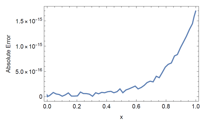
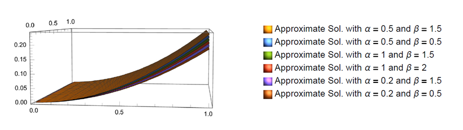
The proposed method demonstrates competitive accuracy, achieving machine precision for \(x \le 0.5\), while maintaining comparable or superior accuracy to Refs. [22,23] across the domain. Figure 1 shows the approximate error at \(N=5\), \(\alpha=2\), and \(\beta=1\). Figure 2 shows the approximate solution at \(N = 3\) with various values of \(\alpha\) and \(\beta\), where \(g(x)\) is adjusted accordingly for each fractional order pair to maintain the exact solution.
Example 2 (Non-periodic transcendental fractional target tracking model). We consider a variation of the nonlinear model introduced in [23]:
subject to \(v(0)= 1 ,\, v'(0)=0\). The exact solution is \(v(x)=\cos{x}\). The absolute errors at integer-order limit \((\alpha=2,\, \beta=1,\, N=5)\) are recorded in Table 2 against the results in [23]. The proposed algorithm reveals dramatic improvement in accuracy, yielding errors near \(10^{-16}\) compared to the \(10^{-6}\) \(\approx\) \(10^{-6}\) range. In Table 3, we document the absolute error patterns across decreasing values of N \((N=4,3,2,1)\) and (\(\alpha=2\), \(\beta=1\)).
| \(x\) | Our method | Method in [23] |
|---|---|---|
| 0.1 | \(3.20924\times10^{-17}\) | \(3.9380\times10^{-6}\) |
| 0.2 | \(7.63278\times10^{-17}\) | \(9.2710\times10^{-6}\) |
| 0.3 | \(1.04083\times10^{-16}\) | \(1.1147\times10^{-6}\) |
| 0.4 | \(1.52656\times10^{-16}\) | \(1.0251\times10^{-5}\) |
| 0.5 | \(1.2490\times10^{-16}\) | \(6.9675\times10^{-5}\) |
| 0.6 | \(8.32667\times10^{-17}\) | \(3.0442\times10^{-6}\) |
| 0.7 | \(8.32667\times10^{-16}\) | \(7.4005\times10^{-6}\) |
| 0.8 | \(1.66533\times10^{-16}\) | \(4.0632\times10^{-6}\) |
| 0.9 | \(1.66533\times10^{-16}\) | \(6.0542\times10^{-6}\) |
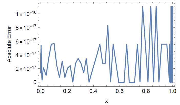
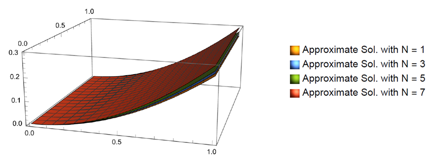
Crucially, Table 4 outlines the Maximum Absolute Errors (MAEs) across various fractional configurations \((\alpha \in \{0.4,0.9,1.4 \},\, \beta \in \{0.2,0.5,0.8 \})\), proving that the algorithm remains immune to numerical errors when handling non-integers. We acknowledge that the repeated error values at the level of \(10^{-16}\) to \(10^{-17}\) indicate that the method has reached the machine precision limit of the arithmetic operations, rather than representing a distinct discretization error. The method exhibits high accuracy and general stability, though minor nonmonotonicity in \(N\) can occur due to the interplay of round-off errors and the conditioning of the nonlinear solver at machine precision. Figure 3 shows the approximate error at \(N=4\), \(\alpha=0.8\), and \(\beta=1.4\). Figure 4 shows the approximate solution via different values of N.
| \(x\) | N = 4 | N = 3 | N = 2 | N = 1 |
|---|---|---|---|---|
| 0.1 | \(1.73472\times10^{-18}\) | \(1.73472\times10^{-18}\) | \(8.67362\times10^{-19}\) | \(1.52\times10^{-2}\) |
| 0.2 | \(0\) | \(6.93889\times10^{-18}\) | \(6.93889\times10^{-18}\) | \(3.01\times10^{-2}\) |
| 0.3 | \(0\) | \(2.77556\times10^{-17}\) | \(2.08167\times10^{-17}\) | \(4.45\times10^{-2}\) |
| 0.4 | \(4.16334\times10^{-17}\) | \(4.16334\times10^{-17}\) | \(2.77556\times10^{-17}\) | \(5.80\times10^{-2}\) |
| 0.5 | \(5.55112\times10^{-17}\) | \(0\) | \(2.77556\times10^{-17}\) | \(7.02\times10^{-2}\) |
| 0.6 | \(1.38778\times10^{-16}\) | \(8.32667\times10^{-17}\) | \(8.32667\times10^{-17}\) | \(8.10\times10^{-2}\) |
| 0.7 | \(0\) | \(2.77556\times10^{-17}\) | \(2.77556\times10^{-17}\) | \(9.01\times10^{-2}\) |
| 0.8 | \(5.55112\times10^{-17}\) | \(5.55112\times10^{-17}\) | \(5.55112\times10^{-17}\) | \(9.75\times10^{-2}\) |
| 0.9 | \(5.55112\times10^{-17}\) | \(0\) | \(5.55112\times10^{-17}\) | \(1.03\times10^{-1}\) |
| N = 2 | N = 3 | N = 4 | N = 5 | N = 6 | ||
|---|---|---|---|---|---|---|
| \(\alpha=0.4\) | \(\beta=0.2\) | \( 3.33067\times10^{-16 }\) | \( 1.11022\times10^{-16 }\) | \( 1.11022\times10^{-16 }\) | \( 1.55431\times10^{-15 }\) | \( 1.66533\times10^{-15 }\) |
| \(\beta=0.5\) | \( 8.32667\times10^{-17 }\) | \( 2.22045\times10^{-16 }\) | \( 2.77556\times10^{-16 }\) | \( 8.32667\times10^{-16 }\) | \( 1.72085\times10^{-15 }\) | |
| \(\beta=0.8\) | \( 4.44089\times10^{-16 }\) | \( 1.9984\times10^{-15 }\) | \( 1.11022\times10^{-16 }\) | \( 4.996\times10^{-16 }\) | \( 1.11022\times10^{-16 }\) | |
| \(\alpha=0.9\) | \(\beta=0.2\) | \( 2.77556\times10^{-16 }\) | \( 2.22045\times10^{-16 }\) | \( 1.66533\times10^{-16 }\) | \( 3.33067\times10^{-16 }\) | \( 9.99201\times10^{-16 }\) |
| \(\beta=0.5\) | \( 1.11022\times10^{-16 }\) | \( 2.22045\times10^{-16 }\) | \( 8.32667\times10^{-17 }\) | \( 1.66533\times10^{-16 }\) | \( 9.4369\times10^{-16 }\) | |
| \(\beta=0.8\) | \( 2.22045\times10^{-16 }\) | \( 2.22045\times10^{-16 }\) | \( 7.77156\times10^{- 16}\) | \( 2.33147\times10^{-15 }\) | \( 6.99441\times10^{-15 }\) | |
| \(\alpha=1.4\) | \(\beta=0.2\) | \( 1.11022\times10^{-16 }\) | \( 2.22045\times10^{-16 }\) | \( 9.99201\times10^{-16 }\) | \( 5.55112\times10^{-16 }\) | \( 1.66533\times10^{-16 }\) |
| \(\beta=0.5\) | \( 1.11022\times10^{-16 }\) | \( 5.55112\times10^{-17 }\) | \( 1.11022\times10^{-16 }\) | \( 1.11022\times10^{-16 }\) | \( 1.11022\times10^{-16 }\) | |
| \(\beta=0.8\) | \( 1.11022\times10^{-16 }\) | \( 2.22045\times10^{-16 }\) | \( 1.11022\times10^{-16 }\) | \( 5.55112\times10^{-17 }\) | \( 5.55112\times10^{-17 }\) |
Example 3 (Cubic-Quintic-Heptic nonlinear polynomial models [23]). Consider the following nonlinear equation with constraints \(v(0)= 1 ,\, v'(0)=0\)
The analytic solution is \(v(x)=1+x^3\). We note that since the exact solution \(v(x) = 1+x^3\) is a polynomial of degree 3, it is exactly contained in the approximation space for \(N \ge 1\). Thus, the machine-level accuracy observed here demonstrates the polynomial exactness of the method, serving as a successful verification of the implementation. The invariant error across different nonlinear cases is a consequence of the solution being exactly represented in the basis, with the residual error dominated by the fixed machine precision limit of the arithmetic operations rather than the nonlinearity itself. For the integer-order limiting cases, the fractional orders are assigned the values \(\alpha=2\), \(\beta=1\), and \(N=3\). We investigate three distinct integer-order case studies associated with Example 3:
Case I. f = 2, h = 1, c = 8 , m = 0, e = 0 (Cubic Nonlinearity).
Case II. f = 2, h = 1, c = 8 , m = 2, e = 0 (Cubic-Quintic Nonlinearity).
Case III. f = 2, h = 1, c = 8 , m = 2, e = 3 (Cubic-quintic-Heptic Nonlinearity).
| Case | I | II | III | |||
|---|---|---|---|---|---|---|
| \(x\) | Our method | Method in [23] | Our method | Method in [23] | Our method | Method in [23] |
| 0.1 | \(1.06035\times10^{-16}\) | \(2.54144\times10^{-18}\) | \(1.06035\times10^{-16}\) | \(1.65877\times10^{-17}\) | \(1.06035\times10^{-16}\) | \(3.87176\times10^{-18}\) |
| 0.2 | \(1.73472\times10^{-17}\) | \(6.61306\times10^{-18}\) | \(1.06035\times10^{-16}\) | \(5.70251\times10^{-17}\) | \(1.06035\times10^{-16}\) | \(1.45989\times10^{-17}\) |
| 0.3 | \(8.32667\times10^{-17}\) | \(6.88578\times10^{-18}\) | \(1.06035\times10^{-16}\) | \(1.07323\times10^{-16}\) | \(1.06035\times10^{-16}\) | \(3.08491\times10^{-17}\) |
| 0.4 | \(6.93889\times10^{-17}\) | \(1.96947\times10^{-18}\) | \(1.06035\times10^{-16}\) | \(1.53493\times10^{-16}\) | \(1.06035\times10^{-16}\) | \(5.12900\times10^{-17}\) |
| 0.5 | \(1.38778\times10^{-17}\) | \(2.52818\times10^{-17}\) | \(1.06035\times10^{-16}\) | \(1.81547\times10^{-16}\) | \(1.06035\times10^{-16}\) | \(7.45896\times10^{-17}\) |
| 0.6 | \(0\) | \(6.83802\times10^{-17}\) | \(1.06035\times10^{-16}\) | \(1.77494\times10^{-16}\) | \(1.65877\times10^{-16}\) | \(9.94154\times10^{-17}\) |
| 0.7 | \(5.55112\times10^{-17}\) | \(1.36594\times10^{-16}\) | \(1.06035\times10^{-16}\) | \(1.27348\times10^{-16}\) | \(1.06035\times10^{-16}\) | \(1.24435\times10^{-16}\) |
| 0.8 | \(0\) | \(2.35252\times10^{-16}\) | \(1.06035\times10^{-16}\) | \(1.71176\times10^{-17}\) | \(1.06035\times10^{-16}\) | \(1.48317\times10^{-16}\) |
| 0.9 | \(1.11022\times10^{-16}\) | \(3.69683\times10^{-16}\) | \(1.06035\times10^{-16}\) | \(1.67184\times10^{-16}\) | \(1.06035\times10^{-16}\) | \(1.69728\times10^{-16}\) |
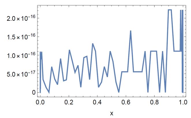
Table 5 presents a comparative analysis of the absolute errors obtained via the proposed method and the technique developed in [23] for \(N=3\), \(\alpha=2\), and \(\beta=1\). A closer inspection of the numerical data reveals that both approaches achieve exceptional precision, with the AEs consistently remaining within the order of \(10^{-16}\) to \(10^{-18}\). In Case (I), the proposed method exhibits highly competitive accuracy; notably, the error completely vanishes (yielding an exact absolute error of zero) at specific nodes such as \(x = 0.6\) and \(x=0.8\), underscoring its superior localized convergence properties. Furthermore, for Cases (II) and (III), the proposed algorithm demonstrates remarkable stability, maintaining a uniform AE of approximately \(1.06035 \times 10 ^{-16}\) across nearly all spatial nodes. In contrast to the fluctuations observed in the results of [23], the steady and invariant error profile of the present method highlights its robust performance and geometric consistency when handling highly nonlinear terms, such as cubic-quintic and cubic-quintic-septic structures. Figure 5 shows the absolute error via \(N=4\), \(\alpha=2\), and \(\beta=1\).
Example 4 (Generalized Liénard equation via hyperbolic solutions [24–26]). We investigate a highly nonlinear Liénard equation explicitly formulated as \(v''(x) + (\beta_1 + \beta_2 v^2(x))v'(x) + \beta_3 v(x) + \beta_4 v^3(x) = 0\), which maps to the generic form with \(\alpha=2, \beta=0\) and specific nonlinear coefficients:
subject to \(v(0)=\frac{1}{\sqrt{2}},\, v'(0)=\frac{\sqrt{2}}{4}\). The analytic solution is \(v(x)=\sqrt{\frac{1+\tanh(x)}{2}}\).
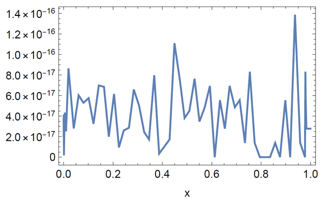
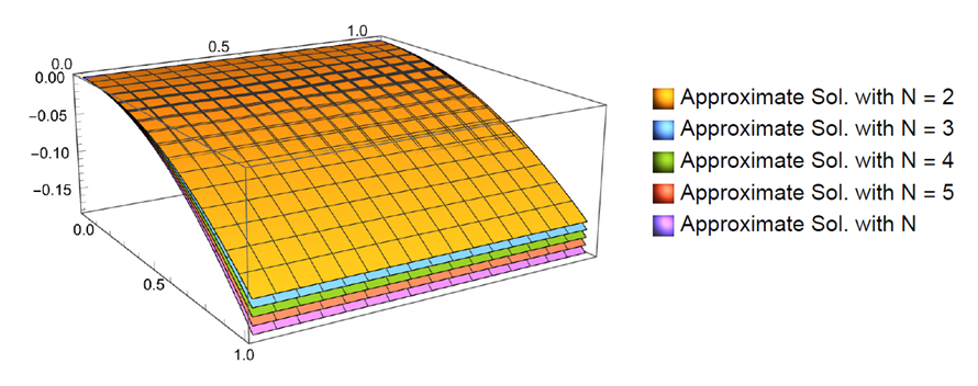
Table 6 presents a comparative validation of the absolute errors (AEs) against three established numerical methods: the differential transform method, a hybrid heuristic computational approach, and an accurate Liénard-solver proposed in [24], [25], and [26]. Operating at a mere fraction of the basis size (N = 6 in the reference literature), the proposed scheme attains an absolute error bound of \(10^{-17}\), outperforming the reference models by up to eleven orders. Figure 6 shows the approximate error at \(N=6\), \(\alpha=2\), and \(\beta=0\). Figure 7 shows the multi-component approximate solutions mapped via different values of N.
| \(x\) | Our method | Method in[25] | Method in[26] | Method in[24] |
|---|---|---|---|---|
| N = 6 | N = 6 | N = 6 | N = 6 | |
| 0.1 | \(6.78711 \times10^{-17}\) | \(2.2683\times10^{-6}\) | \(6.24\times10^{-6}\) | \(6.7141\times10^{-8}\) |
| 0.2 | \(8.06646\times10^{-17}\) | \(2.5222\times10^{-6}\) | \(5.60\times10^{-6}\) | \(1.1401\times10^{-7}\) |
| 0.3 | \(1.9082\times10^{-17}\) | \(1.4404\times10^{-5}\) | \(5.15\times10^{-6}\) | \(1.4010\times10^{-7}\) |
| 0.4 | \(7.28584\times10^{-17}\) | \(6.1806\times10^{-5}\) | \(5.08\times10^{-6}\) | \(1.4855\times10^{-7}\) |
| 0.5 | \(2.08167\times10^{-17}\) | \(2.2099\times10^{-4}\) | \(5.00\times10^{-6}\) | \(1.4131 \times 10^{-7}\) |
| 0.6 | \(1.249\times10^{-16}\) | \(6.5187\times10^{-4}\) | \(4.60\times10^{-6}\) | \(2.6414 \times 10^{-7}\) |
| 0.7 | \(6.93889\times10^{-18}\) | \(1.6408\times10^{-3}\) | \(3.96\times10^{-6}\) | \(4.3610 \times 10^{-7}\) |
| 0.8 | \(1.38778\times10^{-17}\) | \(3.6469\times10^{-3}\) | \(3.39\times10^{-6}\) | \(5.8126 \times 10^{-7}\) |
| 0.9 | \(1.38778 \times10^{-17}\) | \(7.3493\times10^{-3}\) | \(3.15\times10^{-6}\) | \(6.4934 \times 10^{-7}\) |
Example 5 (Highly nonlinear boundary-layer Liénard system). For rigorous test case, we consider a Liénard formulation explicitly defined with its nonlinear functions \(f(y)\) and \(g(y)\) featuring complex irrational coefficients [24–26]:
subjected to \(v(0)= \frac{1}{\sqrt{1+\sqrt{2}}},\, v'(0)=0\). The exact solution is given by the hyperbolic function:
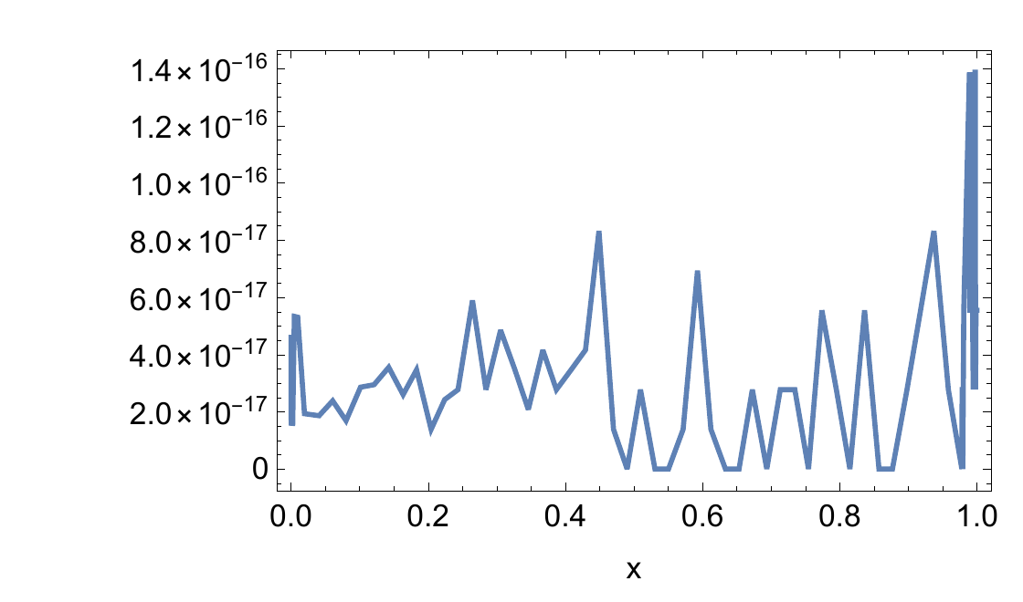
Table 7 verifies the absolute errors under \(N=3\), \(\alpha=2\), and \(\beta=0\). The proposed Delannoy collocation algorithm achieves an error range of \(10^{-17}\), significantly surpassing the precision scales of \(10^{-2}\) \(\approx\) \(10^{-6}\) recorded by alternative methods in [24–26]. Lastly, Table 8 chronicles the relationship between the exact solution, the computed approximate fields, and the corresponding AEs for higher-order expansions (N = 4 and N = 5), validating the structural stability and rapid spectral convergence of our numerical scheme. The spatial distribution of the absolute error for N = 3, \(\alpha=2\), and \(\beta=0\) is illustrated in Figure 8.
| \(x\) | Our method | Method in [25] | Method in [26] (Interior Point Algorithm) |
Method in [26] (Active Set Algorithm) |
Method in [24] |
|---|---|---|---|---|---|
| N = 3 | N = 4 | N = 4 | N = 4 | N = 4 | |
| 0.1 | \(4.0332\times10^{-17}\) | \(4.0668\times10^{-6}\) | \(4.33\times10^{-5}\) | \(1.64\times10^{-5}\) | \(2.5685\times10^{-8}\) |
| 0.2 | \(4.3368\times10^{-17}\) | \(3.7000\times10^{-6}\) | \(5.31\times10^{-5}\) | \(2.22\times10^{-5}\) | \(5.1433\times10^{-7}\) |
| 0.3 | \(1.3878\times10^{-17}\) | \(7.1793\times10^{-6}\) | \(5.84\times10^{-5}\) | \(2.55\times10^{-5}\) | \(1.3397\times10^{-6}\) |
| 0.4 | \(4.1633\times10^{-17}\) | \(6.1806\times10^{-5}\) | \(6.37\times10^{-5}\) | \(2.21\times10^{-5}\) | \(2.3254\times10^{-6}\) |
| 0.5 | \(1.3878\times10^{-17}\) | \(2.4676\times10^{-4}\) | \(6.49\times10^{-5}\) | \(1.54\times10^{-5}\) | \(3.2340\times10^{-6}\) |
| 0.6 | \(1.3878\times10^{-17}\) | \(9.9922\times10^{-4}\) | \(6.01\times10^{-5}\) | \(1.11\times10^{-5}\) | \(3.8973\times10^{-6}\) |
| 0.7 | 0 | \(3.2168\times10^{-3}\) | \(5.27\times10^{-5}\) | \(1.09\times10^{-5}\) | \(4.2577\times10^{-6}\) |
| 0.8 | 0 | \(8.7371\times10^{-3}\) | \(4.67\times10^{-5}\) | \(1.13\times10^{-5}\) | \(4.3703\times10^{-6}\) |
| 0.9 | \(5.5511\times10^{-17}\) | \(2.0841\times10^{-2}\) | \(4.28\times10^{-5}\) | \(7.47\times10^{-6}\) | \(4.3323\times10^{-6}\) |
| \(N=4\) | \(N=5\) | ||||
|---|---|---|---|---|---|
| \(x\) | Exact Sol. | Approximate Sol. | Absolute Error | Approximate Sol. | Absolute Error |
| 0.1 | 0.00374953 | 0.00374953 | \(3.72966\times10^{-17}\) | 0.00374953 | \(1.07336\times10^{-15}\) |
| 0.2 | 0.0147514 | 0.0147514 | \(5.37764\times10^{-17}\) | 0.0147514 | \(2.9126 \times 10^{-15}\) |
| 0.3 | 0.0322654 | 0.0322654 | 0 | 0.0322654 | \(4.56579 \times10^{-15}\) |
| 0.4 | 0.055058 | 0.055058 | \(6.245 \times10^{-17}\) | 0.055058 | \(6.39072 \times10^{-15}\) |
| 0.5 | 0.0814022 | 0.0814022 | 0 | 0.0814022 | \(8.18789 \times10^{-15}\) |
| 0.6 | 0.109077 | 0.109077 | \(5.55112\times10^{-17}\) | 0.109077 | \(1.0103 \times10^{-14}\) |
| 0.7 | 0.13537 | 0.13537 | 0 | 0.13537 | \(1.21292 \times10^{-14}\) |
| 0.8 | 0.157072 | 0.157072 | \(5.55112\times10^{-17}\) | 0.157072 | \(1.48215 \times10^{-14}\) |
| 0.9 | 0.170483 | 0.170483 | \(5.55112 \times10^{-17}\) | 0.170483 | \(1.82077\times10^{-14}\) |
| 1 | 0.171408 | 0.171408 | \(2.77556 \times10^{-17}\) | 0.171408 | \(1.98175\times10^{-14}\) |
In this work, a highly efficient and accurate spectral collocation method based on Delannoy polynomials was successfully developed to solve nonlinear fractional diffusion-type and Liénard ordinary differential equations. By constructing the operational matrices for the Caputo fractional derivative, the governing differential equations were efficiently converted into a system of algebraic equations. Numerical simulations across several benchmark examples demonstrated that the proposed method converges rapidly and achieves high precision (often reaching machine precision limits) with a moderate number of basis functions. Comparative analyses against existing techniques confirmed that the Delannoy framework delivers highly competitive and often more accurate results under comparable settings. Ultimately, these results establish Delannoy polynomials as a powerful, robust, and computationally economical alternative to classical polynomial bases for solving complex fractional-order systems in physics and engineering.
Conflicts of Interest: The authors declare no conflict of interest.
Data Availability: No data is required for this research.
Funding Information: No funding is available for this research.
Acknowledgments: The authors thanks the reviewers and the editor for their careful reading and valuable comments and suggestions.