
1. Introduction
Mathematical models of skeletal muscle serve different purposes and therefore span markedly different levels of resolution. Classical Hill-type models describe the macroscopic force–velocity response using a small number of lumped elements [1,2], whereas Huxley-type and later multiscale models connect whole-muscle behavior to cross-bridge or sarcomere dynamics [3,4]. Three-dimensional continuum and finite-element formulations can represent nonlinear tissue deformation, fiber architecture, active stress, and interactions among muscles [5–7]. Their fidelity is valuable, but parameter identification and computational cost can be substantial, especially when the objective is sensitivity analysis, rapid estimation, or verification of a larger numerical code. Recent reviews consequently emphasize the continuing need for models at several compatible scales rather than a single universally optimal description [8].
The present study addresses a narrower question than a full physiological model: can the spatial and temporal deformation of a tensioned muscle-fiber surrogate, coupled to surrounding tissue, be represented by a mathematically consistent and independently verifiable reduced-order system? This question is relevant to fixed-end and small-transverse-deformation settings in which the dominant output is a displacement field rather than a complete prediction of metabolic activation, force–length behavior, or joint motion. The intended use is therefore a benchmark for analytical reasoning and numerical verification, not direct patient-specific prediction.
The model has four specific contributions. First, the surrounding tissue is represented by an explicit Kelvin–Voigt foundation, so the words “elastic” and “viscous” correspond to identifiable terms in the governing equation. Second, the through-thickness kinematics use the effective tissue depth rather than a ratio that becomes singular at a fixed endpoint. Third, the perturbation hierarchy is solved using fixed-end Fourier modes with the correct mode-dependent damped frequency and Duhamel time convolution. Fourth, the truncated analytical representation is evaluated against an independently discretized finite-difference model, and all dimensionless parameters, numerical tolerances, grid sizes, and errors are reported. These changes make the calculation transparent and reproducible while retaining the compact character of the original fiber-on-foundation concept.
The limitations of this scope are important. Skeletal muscle is an anisotropic, hierarchical, active material that may undergo large three-dimensional deformation [7,9]. A one-dimensional fiber surrogate cannot reproduce pennation, incompressibility, heterogeneous activation, cross-bridge kinetics, intramuscular pressure, or muscle–tendon interaction. The model developed below should thus be interpreted as a mechanically well-posed reduced-order component. Its value depends on stating these restrictions explicitly and validating the mathematics within that restricted domain.
2. Method of solution
Let \(z\in[0,L]\) denote position along a representative fiber and let \(y\in[0,H]\) denote depth measured from the free surface of the effective tissue layer. The transverse displacement of the fiber centerline is \(V(z,t)\). A linear through-thickness reconstruction is adopted,
where \(H>0\) is the effective tissue depth and \(\alpha\) is a bounded correction describing mild departure from uniform through-thickness motion. In contrast with a factor \(y/z\), Eq. (1) remains finite at \(z=0\) and \(z=L\). The reduced equation for \(V\) is obtained by representing the surrounding tissue as a Kelvin–Voigt foundation and the activation-induced action as a distributed load:
here \(m\) is mass per unit fiber length, \(c_s\) is the effective viscous coefficient per unit length, \(k_s\) is the effective foundation stiffness per unit length, \(T\) is the depth-averaged fiber tension, and \(q_a\) is a prescribed activation-related transverse load per unit length. The signs of \(V\) and \(q_a\) are chosen consistently, so a positive \(q_a\) produces positive displacement. Linear Kelvin–Voigt behavior is a controlled small-deformation approximation; time-dependent and nonlinear passive muscle behavior requires a more elaborate constitutive law [10].
The fiber is fixed at both ends,
and contraction is initiated from a compatible quiescent state,
These data remove the endpoint incompatibility produced by combining fixed ends with a nonzero spatially uniform initial displacement.
Spatial heterogeneity of the tension is written as
where \(T_0>0\) is the reference tension. The restriction on \(\varepsilon g\) ensures positive tension. We seek
Substitution of Eqs. (4) and (5) into Eq. (2), followed by collection of equal powers of \(\varepsilon\), gives
and, for \(i\geq1\),
Each order satisfies
For fixed ends, write
Define \(\gamma=c_s/(2m)\), \(\omega_n^2=(T_0k_n^2+k_s)/m\), and \(\Omega_n=(\omega_n^2-\gamma^2)^{1/2}\) for the underdamped case. Projection onto the sine basis and use of Eq. (7) yield
where the source coefficients are
Eqs. (8) and (9) use \(n\geq1\), have the required \(n\)-dependent frequencies, satisfy both initial conditions, and account for the full time history of a nonstationary load. When \(g\) is sufficiently regular, integration by parts converts \(R_{in}\) to a modal coupling matrix without differentiating \(g\) numerically. The approximation used below is \(V^{(2)}=V_0+\varepsilon V_1+\varepsilon^2V_2\).
For transparent numerical testing, introduce
which converts Eq. (2) to
The reported test uses \(\delta=0.35\), \(\kappa=1.0\), \(\varepsilon=0.20\), \(g(x)=\cos(2\pi x)\), and
These are dimensionless verification parameters rather than fitted human or animal tissue properties. Their purpose is to exercise inertia, damping, foundation elasticity, nonuniform tension, and a smooth activation transient simultaneously.
The modal calculation retains 40 sine modes and integrates the coupled order-zero, order-one, and order-two modal systems with an eighth-order adaptive explicit solver using relative and absolute tolerances \(2\times10^{-11}\) and \(2\times10^{-13}\), respectively, and maximum step \(0.004\). The independent reference calculation places Eq. (2) in conservative flux form on 401 uniformly spaced points. It uses centered interface fluxes and the unconditionally stable average-acceleration Newmark method with \(\beta=1/4\), \(\gamma_N=1/2\), and time step \(0.002\) [11]. No modal information is used by the finite-difference calculation. The supplied simulation script regenerates the figure and all reported error measures.
3. Discussion
Figure 1 summarizes the response and validation. Figure 1(a) shows the second-order displacement profiles at \(\tau=1\) for \(q_0=0.50\), \(1.00\), and \(1.50\). The fixed-end conditions are satisfied exactly by the sine basis, and the largest displacement occurs near the fiber midpoint. Because the governing equation is linear for prescribed \(g\), increasing \(q_0\) scales the response without changing its principal spatial pattern. This behavior is a property of the reduced linear problem and should not be extrapolated to large-strain muscle behavior, where material and geometric nonlinearities alter both amplitude and shape.
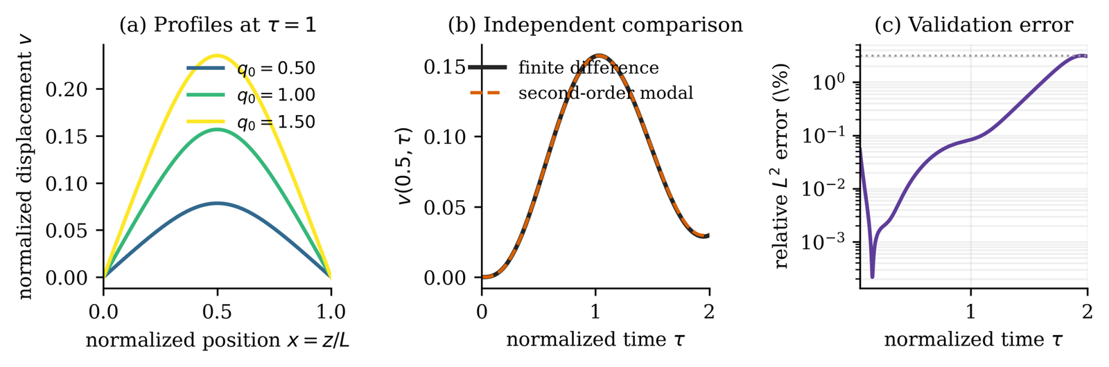
Figure 1(b) provides the essential check that was absent from the original formulation. The second-order modal response and the independently discretized finite-difference result are visually coincident over \(0\leq\tau\leq2\). Their global relative root-mean-square difference is \(4.410\times10^{-3}\), or \(0.441\%\). The maximum absolute difference at the midpoint is \(8.044\times10^{-4}\) in normalized displacement. Figure 1(c) shows that the time-resolved relative \(L^2\) difference remains below \(3.164\%\) after \(\tau=0.05\). The increasing late-time difference is consistent with the neglected \(O(\varepsilon^3)\) and higher coupling terms rather than spatial under-resolution.
The independence and convergence of the reference calculation were checked explicitly. At the final time, changing the finite-difference grid from 101 to 401 points changes the displacement by \(3.257\times10^{-5}\) in relative \(L^2\) norm; changing from 201 to 401 points changes it by only \(6.491\times10^{-6}\). These values are much smaller than the modal-versus-finite-difference difference, supporting the interpretation that the latter is dominated by perturbation truncation. All figures are generated from the stated equations and parameters; no curve is schematic and no unreported fitting is used.
The revised formulation corrects several issues that materially affect reproducibility. The zero-order solution uses a cosine-compatible Green response through the convolution kernel and therefore satisfies zero initial displacement and velocity. The summation starts at \(n=1\), eliminating the undefined zero mode. The eigenfrequency contains \(n\pi/L\), as required by fixed-end separation of variables. Time-dependent forcing is integrated over its history rather than treated as an instantaneous spatial integral. Finally, \(\xi\), rather than the free coordinate \(z\), is used as the integration variable.
The physical interpretation should remain conservative. The Kelvin–Voigt coefficients \(k_s\) and \(c_s\) represent effective transverse restraint and dissipation after reduction of the surrounding tissue; they are not asserted to be universal material constants. Similarly, \(q_a\) is an imposed activation-related load, not a derivation of actomyosin kinetics. Modern three-dimensional formulations include active and passive fiber contributions, large deformation, subject-specific geometry, and experimental calibration [6,7]. The present model instead offers a compact reference problem that can be evaluated rapidly and can test whether more complex solvers recover the expected small-deformation limit.
Experimental validation remains a necessary next step before physiological or clinical use. Appropriate experiments would measure time-resolved displacement under controlled activation while independently estimating geometry, boundary compliance, and loading. The effective parameters could then be identified on a calibration subset and evaluated on held-out conditions. Such data were not available for the present reconstruction, and numerical agreement must not be described as experimental agreement. This distinction prevents overinterpretation while preserving the value of the current verification study.
4. Conclusion
A mathematically consistent reduced-order model has been developed for the transverse deformation of a skeletal-muscle fiber surrogate coupled to viscoelastic surrounding tissue. The model explicitly includes foundation stiffness and damping, uses nonsingular through-thickness kinematics, and imposes compatible initial and boundary conditions. Spatial tension heterogeneity is handled by a bounded perturbation expansion, and the resulting fixed-end Fourier coefficients are expressed with the correct mode-dependent damped Green function and time convolution.
For the stated dimensionless verification problem with \(\varepsilon=0.20\), the second-order approximation agrees with an independent conservative finite-difference/Newmark solution to a global relative root-mean-square difference of \(0.441\%\), while the maximum time-resolved relative \(L^2\) difference after the initial loading interval is \(3.16\%\). Finite-difference grid-refinement errors are at least two orders of magnitude smaller. These results support the use of the second-order solution as a rapid approximation for mild tension heterogeneity over the tested time interval.
The contribution is methodological rather than clinical. The model does not capture three-dimensional architecture, large strain, detailed excitation–contraction coupling, muscle–tendon mechanics, or experimentally calibrated tissue parameters. Future work should fit the effective coefficients to measured displacement or force data, assess several activation patterns and boundary conditions, and quantify the range of \(\varepsilon\) and time over which a prescribed error tolerance is maintained. The complete simulation script accompanying the manuscript provides a reproducible basis for those extensions.
Funding Information: No funding is available for this research.
Conflicts of Interest: The author declares no conflict of interest.
Data Availability: No data is required for this research