
1. Introduction
Compartmental epidemic models provide a transparent connection between biological assumptions and population-level trajectories. Their value, however, depends on more than the formal solution of a system of equations. Every transfer between compartments must have an epidemiological interpretation, the state space must remain nonnegative, delays must be accompanied by complete history functions, and analytical approximations must be checked against a converged numerical solution. These requirements are central to the threshold theory of infectious-disease models [1–3] and to the responsible use of models for public-health interpretation [4,5].
Two features are especially important when the observed case series is an incomplete representation of transmission. First, infection is not instantaneously followed by infectiousness or reporting. A latent interval changes epidemic timing, generation intervals, and the response to interventions. Fixed-delay, distributed-delay, exposed-compartment, and renewal formulations offer different representations of this mechanism [6–8]. These representations are not interchangeable unless their implied residence-time and generation-interval distributions are understood. Second, unreported infections can make a substantial contribution to transmission. Models that separate reported and unreported cases have been used to interpret early outbreak data and to assess how isolation and case ascertainment alter transmission [9–11]. Empirical evidence that infectiousness may be appreciable before or near symptom onset further motivates an explicit early-infectious state [12].
The combination of reporting structure and delay creates several technical risks. A delayed incidence entering the infectious class must correspond to an earlier removal from the susceptible class. If the intervening latent population is not represented, summing the displayed compartments can produce artificial creation or loss of population. A delayed system also requires functions on \([-\tau,0]\), not merely point values at \(t=0\). In addition, an incidence proportional to the difference between two infectious compartments can become negative and violate positive invariance. Such defects cannot be repaired through numerical plotting because they concern the definition of the model itself.
Analytical approximation requires equal care. Replacing unknown trajectories by constant averages can be useful for initialization or short-interval analysis, but the averages of coupled nonlinear compartments remain coupled. They cannot generally be obtained by dividing each initial value by a separate integral. The mean equations must instead be solved simultaneously. Picard iteration supplies a natural functional-correction interpretation because every iterate satisfies the integral form of the delay system, while the difference between consecutive iterates gives a direct convergence diagnostic. On intervals that satisfy a contraction condition, the approximation error is bounded; on longer horizons, the construction can be restarted through the method of steps. Numerical delay solvers remain essential for independent verification, including history interpolation, step refinement, and conservation checks [13].
The present study develops a delay-consistent model that distinguishes susceptible individuals, latent infections, early infectious cases, reported isolated cases, unreported symptomatic cases, and removed individuals. The main contributions are a nonnegative force of infection, an explicit latent accounting identity that restores mass balance, complete history conditions, a derivation of the reproduction number, a coupled average closure, and quantitative comparison of functional-correction iterates with a refined numerical reference. The numerical analysis examines a defined synthetic benchmark rather than fitting an unidentified disease dataset. This distinction is important because predictive calibration would additionally require observation models, uncertainty quantification, and structural and practical identifiability analysis [14,15]. The resulting framework therefore supports transparent mechanistic and numerical investigation while avoiding unsupported disease-specific forecasts.
2. Method of solution
Let \(N_0>0\) denote the demographic equilibrium population. The state variables are \(S(t)\), the number susceptible; \(E(t)\), the number infected but still in the latent interval; \(I(t)\), the number infectious before classification as reported or unreported; \(R(t)\), the number of reported symptomatic cases assumed to be effectively isolated; \(U(t)\), the number of unreported symptomatic infectious cases; and \(Q(t)\), the number removed from infectious states. Reported isolation is an explicit modelling assumption, so \(R\) does not contribute to incidence. Unreported cases transmit with relative infectiousness \(\kappa\geq0\). The nonnegative force of new infection is \[\mathcal{J}(t) =\beta(t)\frac{S(t)}{N_0}\left[I(t)+\kappa U(t)\right], \tag{1}\] where \(\beta(t)\geq0\) has units day\(^{-1}\). The fixed latent duration is \(\tau\geq0\), natural mortality is \(\mu\geq0\), recruitment is \(\Lambda\geq0\), progression from \(I\) to reported and unreported states occurs at rates \(\nu_1\) and \(\nu_2\), and removal rates from \(R\) and \(U\) are \(\eta_R\) and \(\eta_U\), respectively.
An individual infected at time \(t-\tau\) survives natural mortality during latency with probability \(\exp(-\mu\tau)\). The governing system is \[\left. \begin{aligned} \frac{\mathrm dS}{\mathrm dt} &=\Lambda-\mathcal{J}(t)-\mu S(t),\\ \frac{\mathrm dE}{\mathrm dt} &=\mathcal{J}(t)-\mathrm e^{-\mu\tau}\mathcal{J}(t-\tau)-\mu E(t),\\ \frac{\mathrm dI}{\mathrm dt} &=\mathrm e^{-\mu\tau}\mathcal{J}(t-\tau) -(\nu_1+\nu_2+\mu)I(t),\\ \frac{\mathrm dR}{\mathrm dt} &=\nu_1 I(t)-(\eta_R+\mu)R(t),\\ \frac{\mathrm dU}{\mathrm dt} &=\nu_2 I(t)-(\eta_U+\mu)U(t),\\ \frac{\mathrm dQ}{\mathrm dt} &=\eta_R R(t)+\eta_U U(t)-\mu Q(t). \end{aligned}\right\} \tag{2}\]
The latent variable is not an arbitrary additional degree of freedom. It is the accounting functional \[E(t)=\int_{t-\tau}^{t} \mathrm e^{-\mu(t-s)}\mathcal{J}(s)\,\mathrm ds, \tag{3}\] whose derivative gives the second equation of (2). Eq. (3) ensures that infection removed from \(S\) is retained in \(E\) until it either enters \(I\) or is lost through natural mortality. For \(\tau=0\), \(E(t)\equiv0\) and the corresponding delayed flow becomes instantaneous.
For \(\tau>0\), continuous nonnegative history functions \[S(t)=\phi_S(t),\quad I(t)=\phi_I(t),\quad R(t)=\phi_R(t),\quad U(t)=\phi_U(t),\quad Q(t)=\phi_Q(t),\qquad -\tau\leq t\leq0, \tag{4}\] are prescribed, and \(E(0)\) is determined from (3). The histories are assumed bounded, \(\beta\) is nonnegative and piecewise continuous, and all rate parameters are nonnegative. These assumptions make the right-hand side locally Lipschitz in the state variables on bounded subsets, so the method of steps gives a unique local solution. The population identity supplies the bound required to continue that solution.
Indeed, with \[N(t)=S(t)+E(t)+I(t)+R(t)+U(t)+Q(t),\] summing (2) cancels both current and delayed infection flows and gives \[\frac{\mathrm dN}{\mathrm dt}=\Lambda-\mu N(t). \tag{5}\]
If \(\Lambda=\mu N_0\) and \(N(0)=N_0\), then \(N(t)=N_0\) for all \(t\geq0\). More generally, (5) keeps \(N\) bounded by the larger of \(N(0)\) and \(\Lambda/\mu\). Positivity follows from the nonnegative incidence and transition rates together with the integral representation (3): at the boundary of each non-latent compartment, its inflow is nonnegative, while \(E(t)\) is an integral of a nonnegative function. Thus the biologically meaningful region \[\Omega=\left\{(S,E,I,R,U,Q)\in\mathbb{R}_{+}^{6}:N\leq \max\left(N(0),\Lambda/\mu\right)\right\},\] is forward invariant for compatible histories.
For constant baseline transmission \(\beta(t)=\beta_0\) and \(\Lambda=\mu N_0\), the disease-free equilibrium is \((N_0,0,0,0,0,0)\). Write \[q=\nu_1+\nu_2+\mu,\qquad h_U=\eta_U+\mu.\]
A newly infected individual survives latency with probability \(\mathrm e^{-\mu\tau}\), remains in \(I\) for mean duration \(1/q\), and enters \(U\) with probability \(\nu_2/q\). While in \(U\), the individual remains infectious for mean duration \(1/h_U\) with relative infectiousness \(\kappa\). The resulting invasion reproduction number is \[\mathcal{R}_0 =\mathrm e^{-\mu\tau}\frac{\beta_0}{q} \left(1+\frac{\kappa\nu_2}{h_U}\right). \tag{6}\]
This expression is the integral of the infection-age kernel and therefore gives the threshold for invasion of the disease-free state [2,3]. For a time-varying transmission rate, the corresponding instantaneous susceptible-adjusted indicator is \[\mathcal{R}_{e}(t) =\frac{S(t)}{N_0}\, \mathrm e^{-\mu\tau}\frac{\beta(t)}{q} \left(1+\frac{\kappa\nu_2}{h_U}\right). \tag{7}\]
It is used here as a transparent intervention diagnostic, not as a substitute for fitting a time-varying renewal model to data.
To formulate the analytical approximation, set \[\boldsymbol{x}(t)=(S,E,I,R,U,Q)^{\mathsf T}, \qquad \boldsymbol{x}'(t) =\boldsymbol{F}\!\left(t,\boldsymbol{x}(t), \boldsymbol{x}(t-\tau)\right),\] where \(\boldsymbol{F}\) is defined by (2). On an interval \([0,H]\), a constant mean vector \(\boldsymbol{a}\) must satisfy the coupled closure \[\boldsymbol{G}(\boldsymbol{a}) := \boldsymbol{a}-\boldsymbol{x}(0) -\frac{1}{H}\int_0^H(H-s) \boldsymbol{F}\!\left(s,\widetilde{\boldsymbol{a}}(s), \widetilde{\boldsymbol{a}}(s-\tau)\right)\mathrm ds =\boldsymbol{0}, \tag{8}\] where \(\widetilde{\boldsymbol{a}}(s)=\boldsymbol{a}\) for \(s>0\) and equals the prescribed history for \(s\leq0\). Because incidence contains \(a_S(a_I+\kappa a_U)\), Eq. (8) is nonlinear and coupled. It is solved simultaneously by a damped Newton iteration subject to nonnegativity; independent denominator formulas are not algebraically valid.
Using the mean closure as the zeroth iterate, define the functional corrections \[\boldsymbol{x}^{[0]}(t)=\boldsymbol{a},\] \[\begin{aligned} \boldsymbol{x}^{[m+1]}(t) &=\boldsymbol{x}(0)+\int_0^t \boldsymbol{F}\!\left( s,\widetilde{\boldsymbol{x}}^{[m]}(s), \widetilde{\boldsymbol{x}}^{[m]}(s-\tau) \right)\mathrm ds,\qquad m\geq0, \end{aligned}\tag{9}\] \[\overline{\boldsymbol{c}}^{[m+1]} =\frac{1}{H}\int_0^H \left[\boldsymbol{x}^{[m+1]}(t) -\boldsymbol{x}^{[m]}(t)\right]\mathrm dt. \tag{10}\]
The first and second analytical approximations are \(\boldsymbol{x}^{[1]}\) and \(\boldsymbol{x}^{[2]}\). The average correction (10) is a convergence diagnostic rather than an independently selected model parameter. If \(\boldsymbol{F}\) is Lipschitz in its current and delayed states with constant \(L\) on \(\Omega\), then the Picard map is a contraction on a step of length \(\Delta\) whenever \(r=2L\Delta<1\). On such a step, \[\left\|\boldsymbol{x}-\boldsymbol{x}^{[m]}\right\|_{\infty} \leq \frac{r^{m}}{1-r} \left\|\boldsymbol{x}^{[1]}-\boldsymbol{x}^{[0]}\right\|_{\infty}. \tag{11}\]
Long intervals are treated by restarting (9) through the method of steps. This local construction is important: a low-order correction should not be assumed accurate over an entire epidemic without an error check.
The numerical benchmark uses \(N_0=1{,}000{,}000\) and a demographic rate \(\mu=(75\times365)^{-1}=3.6529680\times10^{-5}\) day\(^{-1}\), with \(\Lambda=\mu N_0\). The baseline values are \[\left. \begin{gathered} \tau=4,\quad \kappa=0.65,\quad \nu_1=0.13,\quad \nu_2=0.07,\\ \eta_R=0.10,\quad \eta_U=\frac{1}{7},\quad \beta_0=0.3338428943, \end{gathered}\right\} \tag{12}\] with all rates expressed per day. Thus the mean duration in \(I\) is approximately five days, the reporting fraction among classified cases is \(\nu_1/(\nu_1+\nu_2)=0.65\), and (6) gives \(\mathcal{R}_0=2.20\). Constant histories are used on \([-\tau,0]\). Compatibility with (3) and \(N(0)=N_0\) gives \[\left. \begin{aligned} S(0)&=999{,}911.266823,& E(0)&=48.733177,\\ I(0)&=30,&R(0)&=0,\\ U(0)&=10,&Q(0)&=0. \end{aligned}\right\} \tag{13}\]
The controlled scenario uses \[\beta_c(t)=\beta_0 \begin{cases} 1, & t<35,\\ 1-0.60(t-35)/7, & 35\leq t<42,\\ 0.40, & t\geq42. \end{cases} \tag{14}\]
The \(60\%\) change is an illustrative transmission perturbation and is not assigned to a particular intervention. Delay sensitivity is evaluated at \(\tau=0,4,8\) days while recomputing \(\beta_0\) from (6) so that \(\mathcal{R}_0=2.20\) remains fixed. Reporting sensitivity is evaluated at reporting fractions \(0.40\), \(0.65\), and \(0.85\), holding \(\nu_1+\nu_2=0.20\) and the baseline \(\beta_0\) fixed.
The delay system is integrated for 180 days using a fixed-step fourth-order Runge–Kutta method of steps with linear interpolation of delayed states and a production step of \(0.025\) day. A \(0.00625\)-day trajectory is used as the refinement reference. At step sizes \(0.10\), \(0.05\), \(0.025\), and \(0.0125\) day, the maximum incidence discrepancies from the reference are, respectively, \(4.443\times10^{-4}\), \(1.098\times10^{-4}\), \(2.613\times10^{-5}\), and \(5.227\times10^{-6}\) infections per \(100{,}000\) persons per day. Functional corrections are independently compared with the refined numerical solution on a one-day interval. The scaled error is \[\varepsilon_m =\max_j\frac{ \max_{0\leq t\leq1} \left|x_j^{[m]}(t)-x_j^{\mathrm{ref}}(t)\right|} {\max\left(1,\max_{0\leq t\leq1} \left|x_j^{\mathrm{ref}}(t)\right|\right)}. \tag{15}\]
All calculations and the figure are generated by the accompanying simulate_epidemic.py file.
3. Discussion
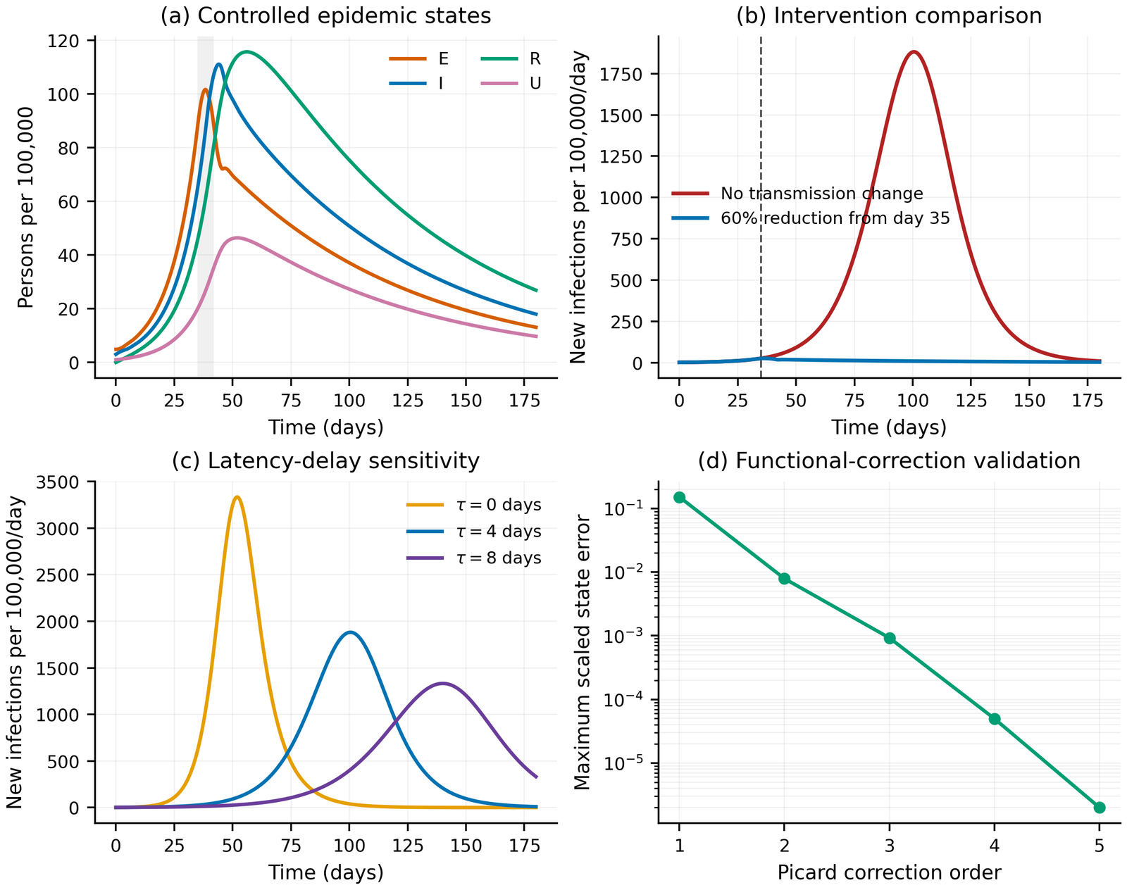
Figure 1 summarizes the model dynamics and validation. The controlled benchmark remains nonnegative in every compartment, and the maximum absolute discrepancy from the population identity (5) is \(6.98\times10^{-9}\) persons across all reported simulations. This residual is at floating-point scale and confirms that current incidence, latent occupancy, delayed progression, and removal have been implemented as internal transfers. It also distinguishes the present construction from a four-state delay system in which the susceptible loss and delayed infectious gain do not balance.
Without a transmission change, incidence reaches \(1881.58\) infections per \(100{,}000\) persons per day on day \(100.50\). The maximum early-infectious prevalence is \(9018.55\) per \(100{,}000\), and cumulative infection through day 180 is \(84.35\%\). These values describe the specified synthetic parameter set; they are not estimates for a real population. Under (14), incidence reaches its maximum of \(25.93\) per \(100{,}000\) per day at the start of the transmission ramp on day 35, while early-infectious prevalence peaks at \(111.13\) per \(100{,}000\). The day-42 value of \(\mathcal{R}_{e}(t)\) is \(0.876\), and cumulative infection through day 180 is \(1.678\%\). Relative to the no-change scenario, the peak incidence and cumulative infection are reduced by approximately \(98.62\%\) and \(98.01\%\), respectively. These differences follow from a defined change in \(\beta(t)\); they should not be interpreted as a universal effect size for an unspecified public-health measure.
Delay sensitivity is examined at a common \(\mathcal{R}_0\) to separate timing from initial invasion potential. With \(\tau=0\), incidence peaks on day \(51.95\) at \(3334.63\) per \(100{,}000\) per day. At \(\tau=4\) days, the peak occurs on day \(100.50\) at \(1881.58\), whereas \(\tau=8\) days moves the peak to day \(140.08\) and reduces it to \(1332.50\). The longer fixed delay therefore slows generation turnover and spreads incidence over a longer period even when the expected number of secondary infections is held constant. Cumulative infection at day 180 is \(84.44\%\), \(84.35\%\), and \(79.03\%\) for zero-, four-, and eight-day delays. The lower value in the eight-day run is partly a finite-horizon effect because its epidemic tail has not ended by day 180; it should not be reported as a general final-size reduction.
Reporting sensitivity has a distinct mechanism. At fixed \(\beta_0\), increasing the reporting fraction transfers more individuals from \(I\) to isolated \(R\) and fewer to transmitting \(U\). When the reporting fraction is \(0.40\), \(\mathcal{R}_0=2.580\), peak incidence is \(2369.50\) per \(100{,}000\) per day on day \(88.93\), and cumulative infection is \(90.33\%\). At a reporting fraction of \(0.85\), these quantities become \(1.896\), \(1438.73\) on day \(114.60\), and \(76.04\%\). The direction of change is epidemiologically interpretable because \(U\) contributes positively to (1). Its magnitude depends on the assumption that reported cases cease transmission; incomplete or delayed isolation would require an additional contribution from \(R\).
The functional-correction validation in Figure 1(d) shows that approximation order must be linked to interval length. On the one-day interval, \(\varepsilon_1=1.521\times10^{-1}\) and \(\varepsilon_2=7.922\times10^{-3}\). The third-, fourth-, and fifth-order errors are \(9.260\times10^{-4}\), \(4.976\times10^{-5}\), and \(1.994\times10^{-6}\). The second correction is therefore accurate to below \(0.8\%\) under the scaled metric for this local interval, but it is not assumed to be globally accurate over 180 days. Restarting the iteration and checking (10) or (15) are necessary on later steps. This explicit validation replaces a qualitative assertion that second order is always sufficient.
The benchmark also clarifies the limits of the evidence. No surveillance, clinical, or individual-level data are analyzed, so the experiment supports mathematical consistency and numerical behavior rather than empirical predictive accuracy. Homogeneous mixing, a fixed latency, constant classification and removal rates, immediate isolation of reported cases, and a single relative infectiousness parameter are simplifying assumptions. A disease-specific analysis would require an observation model linking \(\nu_1 I\) to reported incidence, a likelihood appropriate to count overdispersion, estimation of history and time-varying transmission, and profile-likelihood or Bayesian assessment of identifiability and uncertainty [5,14,15]. Age structure, spatial coupling, vaccination, disease-associated mortality, and distributed residence times could then be added only if the data support the additional parameters. The fixed-delay representation is most appropriate when latency is narrowly distributed; Erlang or renewal formulations are preferable when its variance is material [6,8].
4. Conclusion
A population-consistent delay model has been established for infectious-disease dynamics with latent infection, early infectiousness, reported isolation, and unreported transmission. The formulation supplies the required delay history, uses nonnegative incidence, preserves demographic mass, and yields an explicit reproduction number. The analytical treatment retains the idea of functional corrections but replaces independent average formulas with a coupled closure and a convergent Picard construction. Numerical refinement, conservation, positivity, intervention, delay, reporting, and approximation-error checks are reported with complete parameter values and reproducible code. The synthetic results show how latency can delay and flatten an epidemic at fixed \(\mathcal{R}_0\), how effective reporting can reduce transmission when reported cases are isolated, and how a defined reduction in \(\beta(t)\) can bring \(\mathcal{R}_{e}(t)\) below unity. Empirical forecasting remains outside the scope of the benchmark and should be undertaken only after calibration, identifiability analysis, and uncertainty propagation with a specified disease dataset.
Author Contributions: All authors contributed equally to this paper.
Funding Information: No funding is available for this research.
Conflicts of Interest: The authors declare no conflict of interest.
Data Availability: No human-participant or surveillance data were used. The complete simulation code and the generated numerical metrics accompany the manuscript.