
Modeling fluid dynamics with fractional operators is an active field today, driven by advances in fractional calculus. This interest reflects the ability of fractional calculus to describe memory effects in transport and constitutive relations. Applications to linear viscoelasticity [1] and anomalous diffusion [2] provide relevant mathematical background for the fluid model considered here. The Riemann–Liouville integral and derivative are classical operators in fractional calculus. Unlike the ordinary derivative, the Riemann–Liouville derivative of a nonzero constant is generally nonzero, which can complicate its interpretation in particular physical models. Another distinction concerns the formulation of initial conditions: Riemann–Liouville equations naturally involve fractional initial data, whereas many physical problems prescribe ordinary initial values. Zero initial conditions are not intrinsically excluded by the Riemann–Liouville formulation. The Caputo derivative provides an alternative formulation that accommodates ordinary initial values and is therefore convenient for the present model [3,4]. This derivative is widely used in fractional models with prescribed ordinary initial values and remains an established choice in the literature. The Caputo derivative [3–5] accounts for memory in modeling and is used in differential equations. In the present paper, we use this derivative to describe the temporal evolution of the fluid model. Modeling fluid dynamics with fractional differential equations is well represented in the literature; see, for example, the following papers [6,7]. The classical Caputo derivative has a weakly singular power-law kernel, which represents a particular form of temporal memory. Alternative operators with nonsingular kernels have also been proposed, including the Atangana-Baleanu derivative [8] and the Caputo-Fabrizio derivative [9]. These alternative operators have been applied to various physical problems, although their suitability depends on the intended memory law and the assumptions of the model.
In the present paper, we model the fluid using the Caputo derivative and propose a solution. Several methods are available in the literature for constructing solutions. Numerical approaches include appropriately adapted Runge–Kutta methods and explicit or implicit schemes that account for the history dependence of fractional-order differential equations. Such schemes are useful when direct inversion or closed-form calculations become difficult. Analytical techniques are also available for problems whose mathematical structure permits an explicit treatment of the governing equations. We can cite the homotopy perturbation method applied to fractional calculus problems, the use of Laplace transforms [5], and combinations of the Laplace and Fourier sine transforms. In the present problem, we propose a numerical-analytical method. The method first obtains expressions in the Laplace domain and then applies the Tzou inversion formula to approximate their values in the time domain; a related fractional-fluid application is described in [10]. The successive steps of this solution procedure are described explicitly in the paper. Its advantage is that the transformed solution retains an explicit dependence on the model parameters, while numerical inversion provides approximate temperature and velocity profiles for selected times. In this method, we can analyze the influence of the fractional operator’s order because the solution obtained includes the derivative order. We can find many papers in the literature on the modeling of fluids using a fractional operator. In [11], the authors proposed exact solutions for the free-convection flow of a generalized Jeffrey fluid. In that study, the authors use a fractional derivative with a nonsingular kernel to obtain the solution. A related class of operators is examined in [12]; the authors compare the Atangana–Baleanu and Caputo–Fabrizio formulations for a generalized Casson fluid. In [13], Khan et al. investigate heat and mass transfer in second-grade fluids over a vertical plate by comparing the Atangana–Baleanu and Caputo–Fabrizio derivative formulations. In [14], the authors proposed an interesting application of Caputo-Fabrizio derivatives to the MHD free-convection flow of the generalized Walters-B fluid model. In [15], the authors proposed solutions using the Laplace transform applied to fluid dynamics. In [16], Sene proposed the solutions of the fractional fluid model. Further related investigations of fractional convection, heat transfer, and magnetically influenced fluid flow are reported in [7,17–20].
In this paper, we begin the second section by recalling the fractional operator and Laplace transform used in the present investigation. In the third section, we propose a fluid model and use the Caputo derivative to model the fluid under consideration. In the fourth section, we present the solution procedure, which constitutes the main methodological contribution of this paper. The numerical results, graphical illustrations of the main findings, and their discussion are presented in §5. We conclude with remarks on the present problem.
Several integral and differential operators are used in fractional calculus. This section recalls the definitions needed for the present investigation and distinguishes the Riemann–Liouville and Caputo derivatives. The Caputo formulation is particularly convenient here because the model prescribes ordinary initial values. We also recall the Riemann–Liouville integral, which provides the basis for these definitions and is widely used in the construction and analysis of solutions to fractional differential equations.
Definition 1. Let us consider a function \(v:[0,+\infty[\longrightarrow\mathbb{R}\), assumed locally integrable. Its Riemann–Liouville fractional integral [3,4], wherever the following integral exists, is defined by
where \(\Gamma\) denotes the Euler gamma function, and the order \(\alpha\) is a positive real number satisfying \(\alpha>0\).
As previously mentioned, we recall the Riemann-Liouville derivative defined using the previous integral. The following definition specifies the order range used here and clarifies the placement of the ordinary derivative relative to the integral.
Definition 2. [3,4] Let us consider a function \(v:[0,+\infty[\longrightarrow\mathbb{R}\), for which the following expression exists. The Riemann–Liouville fractional derivative [3,4] of order between zero and one is defined by
where \(t>0\), the fractional order satisfies \(\alpha\in(0,1)\), and \(\Gamma\) denotes the Euler gamma function. The stated expression is understood for functions with the regularity required by the integral and derivative.
Unlike the Riemann–Liouville derivative, the Caputo derivative of a constant function is zero. This property and its compatibility with ordinary initial values motivate the following definition for the model considered in this paper.
Definition 3. [3,4] Let us consider a function \(v:[0,+\infty[\longrightarrow\mathbb{R}\), assumed locally absolutely continuous. The Caputo fractional derivative operator [3,4], for which the ordinary derivative is integrated against a power-law kernel, is defined by
where \(t>0\), the fractional order satisfies \(\alpha\in(0,1)\), and \(\Gamma\) denotes the Euler gamma function. The stated expression is understood for functions with the regularity required by the integral and derivative.
We can observe that in this definition of the Caputo derivative, the integer derivative is inside the integral sign, which means that the Caputo derivative of a constant function is zero. To complete this part, we conclude by recalling the following expression for the Laplace transform of the Caputo derivative when the order satisfies \(\alpha\in\left(0,1\right)\) and the transform exists.
This section will focus on recalling the model we previously discussed for the MHD free-convection flow of a generalized second-grade fluid within a porous medium. We commence the modeling process by employing integer-order derivatives, drawing on prior studies to support our approach. This fundamental work is essential for understanding the behavior of fluid dynamics under the influence of magnetic fields and convection in porous structures:
where \(x\in(0,+\infty)\) and \(t>0\). The physical parameters in these equations have the following meanings. The symbol \(\rho\) denotes fluid density, \(\alpha_1\) is the second-grade material coefficient, and \(\mu\) denotes dynamic viscosity. The quantities \(g\) and \(\sigma\) are gravitational acceleration and electrical conductivity, respectively. The parameter \(\beta_T\) denotes the volumetric coefficient of thermal expansion, \(C_p\) is specific heat capacity, \(k\) is thermal conductivity, and \(\kappa\) is the permeability of the porous medium. The imposed magnetic-field strength is \(B_0\), while \(T_\infty\) denotes the ambient temperature. We now introduce the following dimensionless variables:
In this transformation, the kinematic viscosity is \(\nu\), \(U_{0}\) represents the characteristic velocity, and \(\lambda=\frac{\nu}{U^{2}_{0}}\) is the characteristic time scale; the wall temperature is represented by \(T_{w}\). After introducing these transformations, we obtain the following coupled dimensionless differential equations:
The dimensionless parameters appearing in these equations are defined below. These combinations collect the material properties and characteristic scales used to express the governing equations in the simplified form:
The corresponding initial and boundary conditions are specified as follows. At the initial time, both dimensionless fields are taken to vanish throughout the fluid domain:
for \(y>0\). At the wall and in the far field, the boundary conditions are prescribed by
for \(\tau>0\). In the dimensional model, \(v\) denotes velocity; in the dimensionless equations, \(u\) denotes velocity and \(w\) denotes temperature. Table 1 summarizes the principal dimensionless quantities and parameters used in the formulation, allowing the governing equations and subsequent parameter studies to be interpreted consistently.
| Parameters | Descriptions |
|---|---|
| \(Pr_{eff}\) | Effective Prandtl number governing thermal diffusion |
| \(1/K\) | The inverse dimensionless permeability parameter |
| \(Gr\) | The thermal Grashof number |
| \(\beta\) | The dimensionless second-grade material parameter |
| \(M\) | The magnetic parameter |
| \(u\) | The dimensionless velocity of the fluid |
| \(w\) | The dimensionless temperature distribution |
We now begin modeling with the fractional-order derivative. In this paper, we aim to investigate the influence of the fractional-order derivative on both the velocity and temperature distributions. To achieve our objective, we replace the first-order time derivatives on both sides of Eqs. (8)–(9) with Caputo fractional derivatives, while retaining the second-order spatial derivatives. A related fractionalization procedure, using a different temporal kernel, is adopted in [14]. In other words, we combine integer and fractional derivatives in a single model to examine the behavior of solutions generated by this new approach. The resulting system of fractional differential equations is
The initial and boundary conditions remain unchanged and are specified in Eqs. (12)–(17). The condition presented in Eq. (15) implies that the boundary condition can be expressed in polynomial form.
This section provides a detailed description of the procedure used to solve our two model equations. We begin by addressing the equation describing the temperature distribution and then address the velocity of the fluid. We employ the Laplace transform to obtain ordinary differential equations in the spatial coordinate, then apply the Tzou numerical inversion formula [10] to recover approximate time-domain solutions. In this section, we will use the Laplace transform to solve the second-order differential equation in our model. It is essential to consider the initial and boundary conditions, as they are crucial to the solution process. The conditions are as follows:
By applying the Laplace transform to Eq. (20), we obtain the expression \(\bar{w}(0,s) = \frac{1}{s^{2}}\). Next, we apply the Laplace transform to the second equation in our fluid model. Using the zero initial temperature and collecting the transformed terms gives the following equation:
with the transformed wall boundary condition already specified above, namely
Equation (23) is an ordinary second-order differential equation in the spatial variable \(y\), with the fractional order appearing through the Laplace parameter. Imposing the transformed wall condition and decay at infinity gives the following exact Laplace-domain expression:
Different methods can be used to invert this transformed expression, including representations in terms of suitable special functions. In the present calculation, we use a truncated numerical inversion formula. Its finite sum gives an approximation whose accuracy depends on the truncation index \(N\) and the numerical evaluation of the complex transform:
In this section, we derive the Laplace-domain solution of the fractional differential Eq. (18) and describe its subsequent numerical inversion. The initial and boundary conditions considered are defined in the following form:
We repeat the same procedure used for the temperature distribution. The temperature equation is solved first because its transformed solution supplies the thermal forcing term in the velocity equation. We apply the Laplace transform to Eq. (18), and then we obtain the relationships defined by the forms
To simplify the following mathematical expressions, we introduce the auxiliary quantity \(\rho=Ks^{\alpha}+KM+1\), which is used below to write the transformed velocity equation in a more compact form
This is a linear second-order ordinary differential equation in the spatial coordinate. Its solution combines a decaying homogeneous term with a particular term corresponding to the thermal forcing. After imposing decay at infinity, the Laplace-domain expression takes the following form:
Applying the wall boundary condition gives the relation \(A=-B\). We next determine the explicit form of these coefficients by substituting the proposed particular solution into Eq. (31). Collecting the coefficients of the forcing exponential leads to the expression displayed below:
In this study, we propose the approximate solution by applying the inverse Laplace transform. The formula used for this inversion is based on the Tzou formula, which provides a systematic approach for obtaining the desired results.
We complete this section by calculating the dimensionless wall temperature gradient, denoted here by the Nusselt number. This quantity characterizes the wall heat-transfer response under the temperature normalization adopted in the model and is defined by the following expression:
Differentiating the transformed temperature expression in Eq. (25) with respect to the spatial coordinate and evaluating the result at the wall gives the following Laplace-domain expression for the Nusselt number:
The time-dependent Nusselt number can then be approximated using the same Tzou numerical inversion procedure. Applying the formula to its transformed expression gives
Here, the skin-friction quantity \(Sf\) is represented by the negative dimensionless wall velocity gradient. Under this convention, it measures the near-wall velocity response of the model and is defined by the following expression:
The calculation follows the same differentiation and inversion procedure used for the temperature field. We first differentiate the transformed velocity expression and evaluate the resulting gradient at the wall, obtaining the expression shown below:
Substituting the coefficient \(A\) into the wall-gradient expression yields the following transformed quantity, which is evaluated at complex Laplace arguments during numerical inversion:
Rather than seeking a closed-form time-domain representation of this expression, we apply the Tzou numerical inversion formula to the transformed wall-gradient quantity. This procedure gives the following approximation for the time-dependent response:
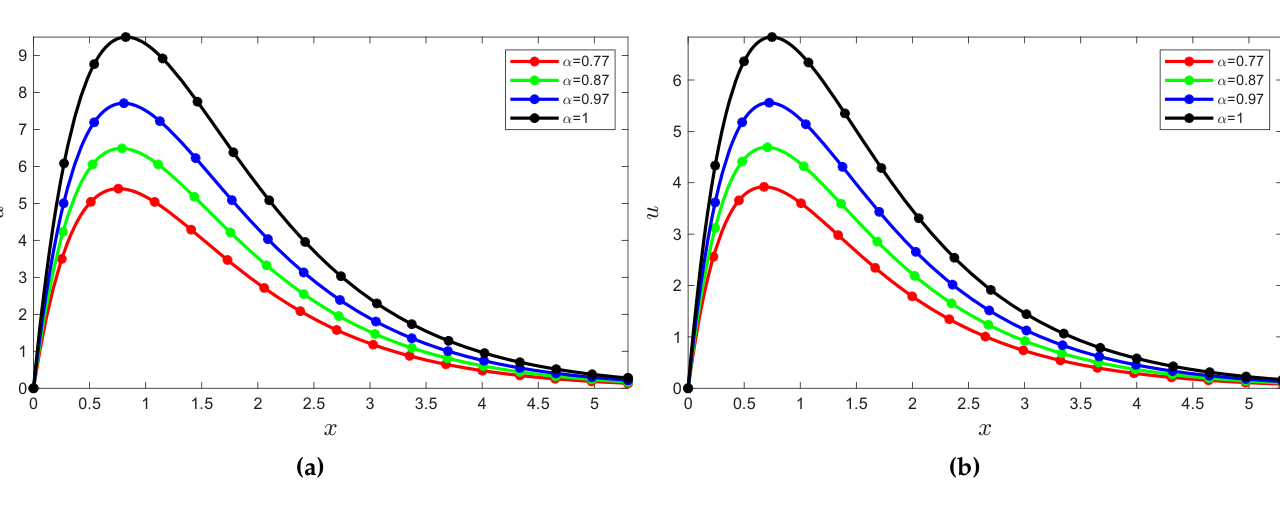
In this section, we will explore the illustration and interpretation of the results. First, we will focus on how the order of the fractional derivative affects the temperature distribution and attempt to explain the observed behavior. A particular objective of this analysis is to present the impact of the effective Prandtl number on the temperature distribution. In the second part, we will analyze the influence of the fractional derivative order on the velocity distribution. Following that, we will examine the impact of the various parameters used in our model to describe velocity. We will begin by analyzing the effect of the effective Prandtl number on our model’s dynamics. For the temperature plots with different effective Prandtl numbers, we set \(\tau=8\) and use the truncation index \(N=18\). Figures 1 and 2 present the results in panels 1a, 1b, 2a, and 2b.
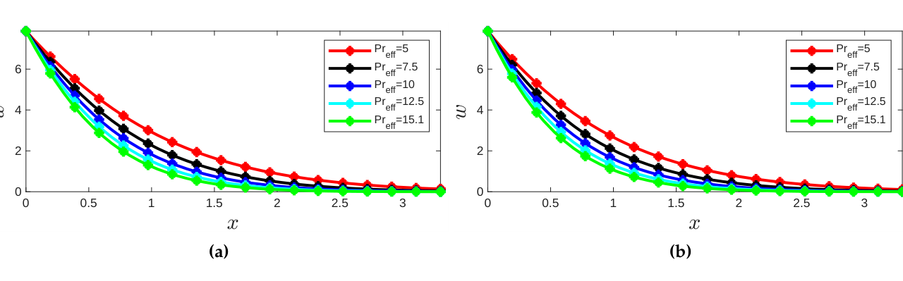
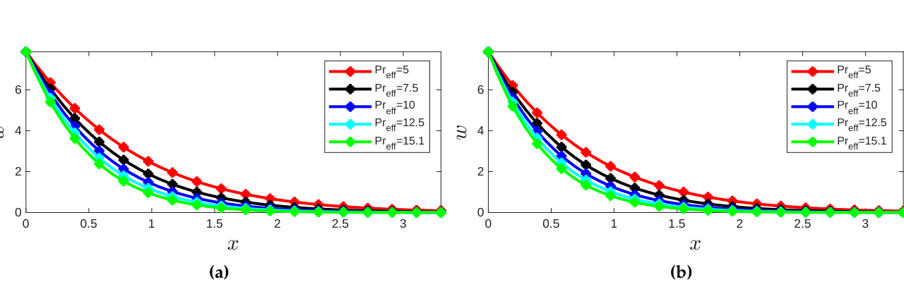
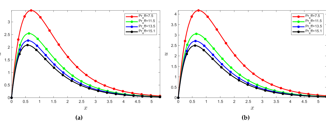
We next examine the temperature profiles obtained by varying the fractional derivative order. Within each panel, the remaining parameters are held fixed so that the influence of the order can be compared directly. Figures 3 and 4 use \(Pr_{eff}=7.5\), \(Pr_{eff}=10.5\), \(Pr_{eff}=12.5\), \(Pr_{eff}=15.1\) successively, as shown in panels 3a,3b,4a,4b.
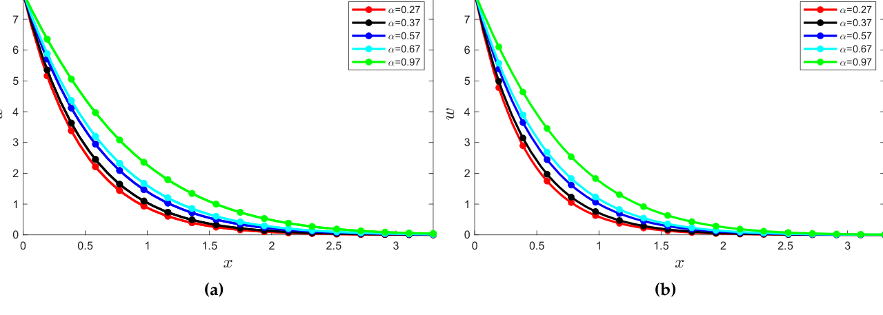
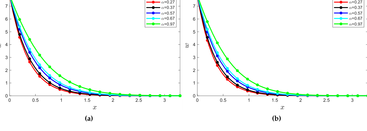
The plotted profiles are used to examine how the Caputo derivative order affects the temperature response. For the parameter choices considered here, the reported curves indicate an increase in temperature with increasing fractional order. This observation concerns the displayed time and parameter values; it should not be interpreted as a universal ordering of all fractional diffusion solutions. Table 2 lists the parameter combinations used for the temperature plots and complements the stated time and truncation index, making the intended numerical comparisons more explicit.
| Orders | Figures | Parameters |
|---|---|---|
| \(\alpha\in\{0.97,0.87\}\) | Panels 1a, 1b. | \(Pr_{eff}\in\left\{5; 7.5; 10; 12.5; 15.1\right\}\) |
| \(\alpha\in\{0.77,0.67\}\) | Panels 2a, 2b. | \(Pr_{eff}\in\left\{5; 7.5; 10; 12.5; 15.1\right\}\) |
| \(\alpha\in\{0.27,0.37,0.57,0.67,0.97\}\) | Panels 3a,3b | \(Pr_{eff}\in\left\{7.5; 10.5\right\}\) |
| \(\alpha\in\{0.27,0.37,0.57,0.67,0.97\}\) | Panels 4a,4b | \(Pr_{eff}\in\left\{12.5; 15.1\right\}\) |
Let us now focus on the variation of the velocity distribution. We begin by examining the impact of the order of the Caputo derivative on the dynamics of the velocity in our model. We set \(Gr=10\), \(M=1\), \(K=1.4\), and \(\beta=1.8\), with the time fixed at \(\tau=8\). Figures 5 and 6, comprising panels 5a, 5b, 6a, and 6b, illustrate the reported influence of the fractional derivative order on the velocity profiles.
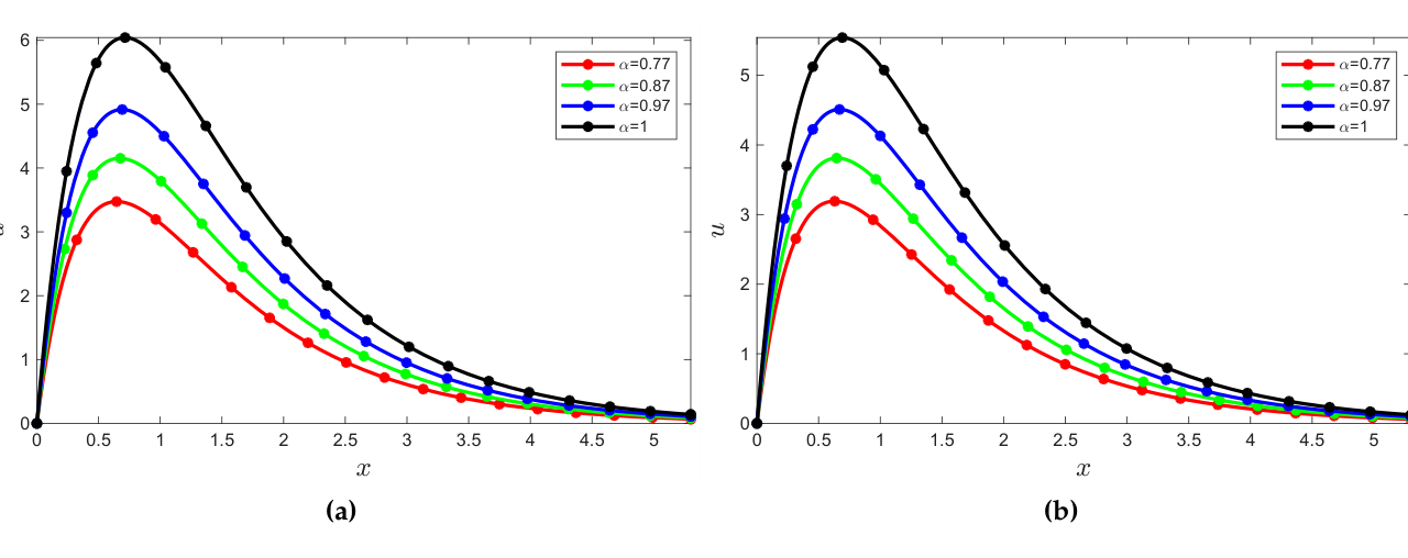
As the fractional order approaches one, the reported velocity profiles increase toward their limiting curves for the displayed parameter choices. The temperature and velocity comparisons therefore show similar trends in this particular calculation. At the operator level, the limit of order one recovers the classical first-order time derivative, linking the fractional description to the corresponding integer-order diffusion model. The effective Prandtl number affects the dynamics of the velocity because the temperature distribution in the model’s constitutive equations influences the constitutive equations for the velocity. We again set \(Gr=10\), \(M=1\), \(K=1.4\), and \(\beta=1.8\), with \(\tau=8\). Figures 7 and 8 compare these velocity profiles in panels 7a, 7b, 8a, 8b.
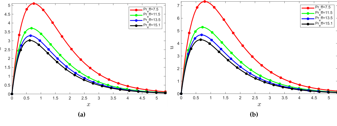
For the parameter choices presented, the reported velocity decreases as the effective Prandtl number increases. This dependence arises through the temperature field: the effective Prandtl number controls the thermal diffusion coefficient, and temperature supplies the buoyancy forcing in the velocity equation.
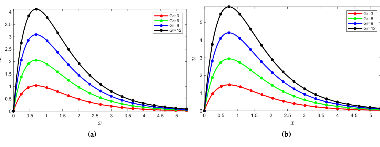
Let us conclude by examining the influence of the \(Gr\) number, which is also important in the diffusion process. We set \(Pr_{eff}=10\), \(M=1\), \(K=1.4\), and \(\beta=1.8\), with the time fixed at \(\tau=8\). For each fixed fractional order, we vary \(Gr\) to obtain the comparisons in Figures 9 and 10, shown in panels 9a, 9b, 10a, 10b.
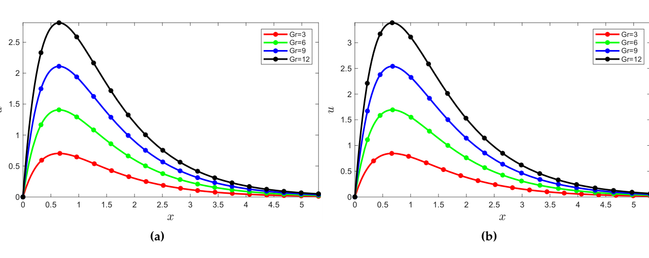
For each fixed fractional order, the reported velocity increases with the Grashof number. This dependence is consistent with the appearance of \(Gr\) as the coefficient multiplying temperature in the buoyancy term of the momentum equation. The fractional order influences the temporal response, whereas varying \(Gr\) changes the strength of thermal forcing. These two effects should therefore be distinguished when interpreting the plotted comparisons.
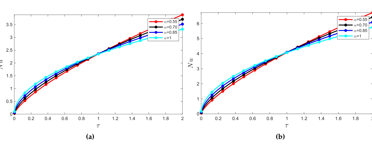
The fractional derivative order and the effective Prandtl number also influence the Nusselt number. Figure 11 illustrates the reported wall heat-transfer response in panels 11a,11b.
The wall velocity-gradient quantity likewise depends on the fractional derivative order and on the parameters \(Gr\), \(K\), \(M\), and \(\beta\). These dependencies follow from the transformed velocity expression and must be considered together when interpreting the near-wall response of the model.
In this paper, we have investigated the MHD free-convection flow model using the Caputo derivative. We applied the Tzou numerical inversion method to obtain approximate temperature and velocity solutions for the fractional fluid model under consideration. We have also analyzed the influence of the order of the fractional derivative; the reported profiles indicate changes in the diffusion response for the times and parameter values considered here. We also analyzed the influence of the effective Prandtl number and the Grashof number on the dynamics of the considered fluid model. It is noticed that an increase in the effective Prandtl number reduces the temperature distribution, and an increase in the Grashof number increases the velocity. The problem outlined in this paper presents opportunities for future research, especially when employing derivatives with a nonsingular kernel. Such extensions would require an explicit choice of memory kernel, a corresponding solution procedure, and a comparison with the present Caputo formulation. They therefore remain topics for future investigation beyond the model analyzed in this paper.
Conflicts of Interest: The author declares no conflicts of interest.
Data Availability: No external datasets were used in this study. The numerical results are derived from the mathematical model and parameter values presented in the paper.
Funding Information: This research received no external funding.