Modelling and simulation of a dynamic contact problem in thermo-piezoelectricity

1. Introduction

The effective conversion of the electrical energy into mechanical energy and vice versa has led the piezoelectric materials to important applications in many engineering structures such as sensors, actuators, intelligent structures, etc. Thermal effects, such as temperature induced deformation and the pyroelectric effect, are especially important for many smart ceramic materials. Thus, a coupling of thermo-electro-mechanical fields is needed to be taken into account if a temperature load is considered in a piezoelectric solid. Models taking into account thermal and piezoelectric effects can be found in [1,2,3].

Thermal effects in contact processes affect the composition and stiffness of the contacting surfaces, and cause thermal stresses in the contacting bodies. When extending contact problems to thermomechanics, additional thermal effects need to be accounted for: heat conduction appears through the contact interface and frictional work is converted to heat. Recent models of frictional contact problems involving thermo-piezoelectric materials can be found in [4,5,6] and the references therein. There, besides the rigorous construction of various mathematical models of contact for thermo-piezoelectric materials, the unique weak solvability of these models was proved, by using arguments of variational and hemivariational inequalities. Numerical analysis of the problems, including numerical simulations, can be found in [7,8]. In [7] the process was assumed to be static, the contact was described with Signorini condition and Tresca's law of dry friction, and a regularized electrical and thermal conductivity conditions and, in [8], the process was assumed to be quasistatic, the contact was assumed to be bilateral, in which contact is always maintained; and associated to the Tresca friction law, and to the heat exchange condition. There, discrete schemes to approximate the problems were considered and implemented in a numerical code, and numerical simulations were provided.

The present paper represents a continuation of [8] and it deals with a mathematical model which describes the frictional contact between a thermo-piezoelectric body and a thermally conductive foundation. We use both the thermo-electro-elastic constitutive law used in [8] but unlike [8], we assume here that the process is dynamic and the foundation is completely rigid and we model the contact with the Signorini condition with Coulomb's law of dry friction. This condition is other physical setting (see, e.g., [9,10]). Also, note that, unlike [8]; here the model includes frictional heat generation and the heat exchange condition, in which the heat exchange coefficient is not a constant but a function of the contact pressure (see [11,12]). The other trait of novelty of the present paper consists in the fact that here we deal with the numerical approach of the problem and provide numerical simulations. The corresponding numerical scheme is based on the spatial and temporal discretization. Furthermore, the spatial discretization is based on the finite element method, while the temporal discretization is based on the Euler scheme. Then, the scheme was utilized as a basis of a numerical code for the problem, in which we develop a specific contact element. We need this element in order to take into account the coupling of the mechanical and thermal unknows on the contact boundary condition. By using the code, simulation results on numerical example are presented.

The rest of paper is structured as follows. In Section 2, we describe our model. Section 3 introduces the variational formulation of the problem, and a fully discrete variational approximation by considering a hybrid formulation. The numerical algorithm used for solving the discrete problem is described in Section 4, where some numerical simulations are also presented to highlight the performance of the method and the effects of the conductivity of the foundation, as well. Finally, in Section 5, we present some conclusions and perspectives.

2. The model

The physical setting is the following: A piezoelectric body occupies a regular domain \(\Omega\subset{\mathbb{R}}^d\,\, (d=2,3) \) with a smooth boundary \(\partial \Omega=\Gamma\). The body is submitted to the action of body forces of density \(\mathbf{f}_{0}\), a volume electric charges of density \(\phi_0\) and a heat source of constant strength \(\vartheta_0 \). It is also submitted to mechanical, electric and thermal constraints on the boundary. To describe them, we consider a partition of \(\Gamma\) into three measurable parts \(\Gamma_D\), \(\Gamma_N\), \(\Gamma_C\), on one hand, and a partition of \(\Gamma_D \cup \Gamma_N\) into two open parts \(\Gamma_a\) and \(\Gamma_b\), on the other hand. We assume that \(meas\,\Gamma_D>0\) and \(meas\,\Gamma_a>0\). The body is clamped on \(\Gamma_D\), therefore, the displacement field vanishes there. Moreover, we assume that a density of traction forces, denoted by \(\mathbf{f}_N\), acts on the boundary part \(\Gamma_N\). We also assume that the electrical potential vanishes on \(\Gamma_a\) and a surface electric charge of density \(\phi_b\) is prescribed on \(\Gamma_b\). We suppose that the temperature vanishes in \(\Gamma_D\cup\Gamma_N\). In the reference configuration, the body is in contact over \(\Gamma_C\) with a thermally conductive foundation. The contact is modelled with a Signorini's conditions and a version of Coulomb's law dry friction. Here, we study the evolution of the state of the system on a finite time interval \([0,T]\), with \(T > 0\). Here and everywhere in this paper \(i, j, k, l\) run from 1 to \(d\), summation over repeated indices is implied and the index that follows a comma represents the partial derivative with respect to the corresponding component of the spatial variable, i.e., \(f_{,i}=\frac{\partial f}{\partial x_i}\).

We denote by \(\mathbf{u} = (u_i) \in\mathbb{R}^d\) the displacement vector, by \(\sigma=(\sigma_{ij})\in \mathbb{S}^d\) the stress tensor, by \(\mathbf{\varepsilon}(\mathbf{u})=(\varepsilon_{ij}(\mathbf{u}))\in \mathbb{S}^d\) the linearized strain tensor, i.e., \(\varepsilon_{ij}(\mathbf{u})=(u_{i,j} + u_{j,i})/2\), by \(\mathbf{E}(\varphi)=-\nabla\varphi= - (\varphi_{,i})\in\mathbb{R}^d\) the electric vector field, where \(\varphi\in\mathbb{R}\) is the electric potential, and by \(\theta\in\mathbb{R}\) the temperature. The notation \(\mathbb{S}^d\) stands for the space of second order symmetric tensors on \(\mathbb{R}^d\). We also use the dot to denote the time derivative, so \(\dot{\mathbf{u}} = (\dot{u}_i)\) represents the velocity vector. The functions \(\mathbf{u}:\Omega\times[0,T]\to\mathbb{R}^d\), \(\sigma:\Omega\times[0,T]\to\mathbb{S}^d\), \(\varphi:\Omega\times[0,T]\to\mathbb{R}\) and \(\theta:\Omega\times[0,T]\to\mathbb{R}\) are the unknowns of the problem, and, for simplicity, we do not indicate the dependence the functions on the variables \(\mathbf{x}\in \Omega\) and \(t\in [0,T]\).

The body is assumed to be thermo-electro-elastic and, therefore, we use the constitutive law

\[\begin{array}{l} \sigma = {\mathcal{F}} \mathbf{\varepsilon}(\mathbf{u}) -{\mathcal{E}}^T \mathbf{E}(\varphi) - \theta\mathcal{M} \quad \hbox{in} \quad \Omega\times(0,T),\\ \mathcal{D}=\mathcal{E}\mathbf{\varepsilon}(\mathbf{u})+\beta \mathbf{E}(\varphi) - \theta\mathcal{P} \qquad \hbox{in} \quad \Omega\times(0,T), \end{array}\] and the heat flux vector \(\mathbf{q} = (q_i) \in\mathbb{R}^d\) is given by the Fourier law of heat conduction \[\mathbf{q} =-\mathcal{K}\nabla\theta \quad \hbox{in} \quad \Omega\times(0,T).\] Here \(\mathcal{D}=(D_i)\) is the electric displacement field and \({\mathcal{F}}=(f_{ijkl})\), \({\mathcal{E}}=(e_{ijk})\), \({{\beta}}=(\beta_{ij})\), \({\mathcal{M}}=(m_{ij})\), \(\mathcal{P}=(p_{i})\) and \(\mathcal{K}=(k_{ij})\) are respectively, the elasticity, piezoelectric, electric permittivity, thermal expansion, pyroelectric and thermal conductivity tensors. \(\mathcal{E}^T\) denotes the transpose of \(\mathcal{E}\); also, the tensors \(\mathcal{E}\) and \(\mathcal{E}^T\) satisfy the equality \({\cal E}\sigma\cdot\mathbf{v}=\sigma\cdot{\cal E}^T\mathbf{v}\;\;\forall\sigma\in\mathbb{S}^d,\, \mathbf{v}\in\mathbb{R}^d\), and the components of the tensor \({\cal E}^T\) are given by \(e_{ijk}^T=e_{kij}\).

Since the process is assumed dynamic, then the equation of stress equilibrium, the equation of the quasistationary electric field, and the heat conduction equation are

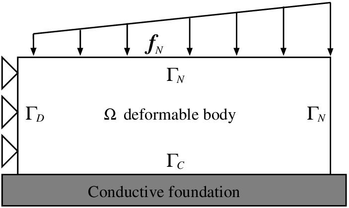
\begin{align*} &\mathcal{D}iv \sigma+ \mathbf{f}_0=\rho\ddot{\mathbf{u}} & \hbox{in} \quad \Omega\times(0,T), \\ &{ \div} \mathcal{D} =\phi_0 & \hbox{in} \quad \Omega\times(0,T), \\ & \theta_{ref}\big(\alpha\dot{\theta} + \mathcal{M}\mathbf{\varepsilon}(\dot{\mathbf{u}}) + \mathcal{P}\mathbf{E}(\dot{\varphi})\big) + {\div} \mathbf{q} =\vartheta_0 & \hbox{in} \quad \Omega\times(0,T). \end{align*} Here \(\alpha\) is given as \(\alpha = \rho c_\nu/\theta_{ref}\), where \(\rho\) is the mass density, \(c_\nu\) is the specific heat and \(\theta_{ref}\) is the reference uniform temperature of the body. Moreover, \(Div\) and \({\div}\) represent the divergence operators for tensor and vector functions, i.e., Div\(\sigma=(\sigma_{ij,j}),\, {\div}\mathcal{Y}=(Y_{i,i})\).

We turn to describe the boundary conditions, so we denote by \(\nu = (\nu_i)\) the unit outward normal on \(\Gamma\). Then, on the \(\Gamma_D\cup\Gamma_N\) portion of the boundary, we impose the following conditions

\[\begin{array}{l} \mathbf{u}=\mathbf{0}\qquad \hbox{on} \quad \Gamma_D\times(0,T),\\ \sigma \nu=\mathbf{f}_N \quad \hbox{on}\quad \Gamma_N\times(0,T). \end{array}\] The boundary conditions for the electric potential can be defined in the following forms: \[\begin{array}{l} \varphi=0 \quad\qquad \hbox{on} \quad \Gamma_a\times(0,T),\\ \mathcal{D}\cdot \nu=\phi_b \quad \hbox{on} \quad \Gamma_b\times(0,T). \end{array}\] Next, on \(\Gamma_D\cup \Gamma_N\) we prescribe a Dirichlet condition for the temperature, say, \[ \theta=0 \quad \hbox{on} \quad \Gamma_D\cup\Gamma_N\times(0,T). \] We now describe the thermo-mechanical boundary conditions on the potential contact surface \(\Gamma_C\). We assume that the normal displacement \(u_\nu=\mathbf{u}\cdot \nu\) and the normal stress \(\sigma_\nu=\sigma\nu\cdot \nu\) satisfy the Signorini's contact conditions \[ u_\nu\leq 0,\quad \sigma_\nu\leq 0,\quad \sigma_\nu u_\nu=0\quad \hbox{on} \quad \Gamma_C\times(0,T). \] The corresponding Coulomb law of dry friction may be stated as follows: \[ \left\{ \begin{array}{l} \mbox{if }\;\dot{\mathbf{u}}_{\tau} = \mathbf{0} \quad \mbox{ then }\quad\|\sigma_{\tau}\| \leq \mu|\sigma_\nu|, \\ \mbox{if }\;\dot{\mathbf{u}}_{\tau} \neq \mathbf{0} \quad \mbox{ then }\quad \sigma_{\tau} = - \mu|\sigma_\nu| \displaystyle\frac{\dot{\mathbf{u}}_{\tau}}{\| {\dot{\mathbf{u}}_{\tau}}\|}, \end{array} \right. \quad \mbox{on}\quad\Gamma_C\times(0,T). \] Here \(\dot{\mathbf{u}}_{\tau} = \dot{\mathbf{u}} - \dot{u}_\nu\nu\) is the tangential velocity, \(\sigma_\tau=\sigma\nu -\sigma_\nu\nu\) represents the tangential force on the contact boundary and \(\mu\geq 0\) is the coefficient of friction.

Next, we describe the boundary condition for the temperature on \(\Gamma_C\). We assume that there is heat exchange between the surface and the foundation, which is at temperature \(\theta_f\). Moreover, since the flux of heat generated by the friction traction on the contact surface is proportional to the tangential shear \(\sigma_\tau\) and to the tangential velocity \(\dot{\mathbf{u}}_\tau\) of the surface, we assume a boundary condition of the following form

\[ \mathbf{q}\cdot \nu = k_c(\sigma_\nu)(\theta - \theta_f) - \mu|\sigma_\nu|\|\dot{\mathbf{u}}_\tau\| \quad \mbox{on} \quad\Gamma_C\times(0,T), \] where \(k_c(\cdot)\) is the normal pressure dependent heat exchange coefficient and has to satisfy \(k_c(0) = 0\). This condition guarantees that there is no heat flux between the body and the foundation if they are not in contact. For \(k_c(\cdot)\), we employ a linear model \(k_c(\sigma_\nu) = \bar{k}_{c}|\sigma_\nu|\), where \(\bar{k}_{c}\geq 0\) is model constant, see [11].

We collect the above equations and conditions to obtain the following mathematical problem.

Problem \(P.\) Find a displacement field \(\mathbf{u}:\Omega\times[0,T]\to\mathbb{R}^d\), a stress field \(\sigma:\Omega\times[0,T]\to\mathbb{S}^d\), an electric potential field \(\varphi:\Omega\times[0,T]\to\mathbb{R}\), an electric displacement field \(\mathbf{D}:\Omega\times[0,T]\to\mathbb{R}^d\), a temperature field \(\theta:\Omega\times[0,T]\rightarrow \mathbb{R}\), and a heat flux \(\mathbf{q}:\Omega\times[0,T]\to\mathbb{R}^d\) such that Here, \(\mathbf{u}_0\), \(\mathbf{v}_0\), \(\varphi_0\) and \(\theta_0\) are the prescribed initial displacement, velocity, electric potential and temperature, respectively.

3. Variational formulation and its approximation

3.1. A hybrid variational formulation

We now turn to the variational formulation of Problem \(P\) which is the starting point for the numerical modelling based on the finite element discretization. We denote in the sequel by \("\cdot"\) and \(\|\cdot\|\) the inner product and the Euclidean norm on the spaces \(\mathbb{R}^d\) and \(\mathbb{S}^d\). We introduce the spaces and we use the notation \(H=[L^2(\Omega)]^d\), and we introduce the spaces \begin{align*} V&=\{\mathbf{w} \in [H^1(\Omega)]^d\, ; \ \mathbf{w}=\mathbf{0} \; \hbox{on} \; \Gamma_D\},\\ W&=\{\xi\in H^1(\Omega)\, ;\, \xi=0 \; \hbox{on} \; \Gamma_a\}, \\ Q&=\{\eta\in H^1(\Omega)\, ;\, \eta=0 \; \hbox{on} \; \Gamma_D\cup\Gamma_N\}, \\ {\cal H}&=\{\tau=(\tau_{ij}) \,; \, \tau_{ij}=\tau_{ji}\in L^2(\Omega) \}. \end{align*} The spaces \(H,\ V,\ W,\ Q\) and \({\cal H}\) are real Hilbert spaces endowed with the canonical inner products given by \begin{align*} &\displaystyle (\mathbf{u},\mathbf{w})_H=\int_\Omega \mathbf{u}\cdot \mathbf{w} \, d\mathbf{x}, \\ &\displaystyle (\mathbf{u},\mathbf{w})_V= \int_\Omega \mathbf{\varepsilon}(\mathbf{u})\cdot \mathbf{\varepsilon}(\mathbf{w}) \, d\mathbf{x}, \\ &\displaystyle (\varphi,\xi)_W=\int_\Omega \nabla\varphi\cdot\nabla\xi\, d\mathbf{x}, \\ &\displaystyle (\theta,\eta)_Q=\int_\Omega \nabla\theta\cdot\nabla\eta\, d\mathbf{x}, \\ &\displaystyle (\sigma,\tau)_{\cal H}=\int_\Omega \sigma\cdot\tau\, d\mathbf{x}. \end{align*} We consider the trace spaces \(X_{\nu}=\{{w_{\nu}}_{|_{\Gamma_C}}\; : \; \mathbf{w}\in V\}\) and \(X_{\tau}=\{{\mathbf{w}_{\tau}}_{|_{\Gamma_C}}\; : \; \mathbf{w}\in V\}\) equipped with their usual norms. Denote respectively by \(X_{\nu}^{*}\) and \(X_{\tau}^{*}\) the dual of the spaces \(X_{\nu}\) and \(X_{\tau}\).

We consider the three mappings \(\mathbf{f} : [0,T]\longrightarrow V\), \(\phi : [0,T]\longrightarrow W\) and \(\vartheta : [0,T]\longrightarrow Q\) defined by

\begin{alignat*}{2} &\displaystyle (\mathbf{f}(t),\mathbf{w})_V=\int_\Omega \mathbf{f}_0(t)\cdot \mathbf{w} \, d\mathbf{x}+ \int_{\Gamma_N} \mathbf{f}_N(t)\cdot \mathbf{w}\, da,\;\;\;\; && \forall \mathbf{w}\in V,\nonumber \\ &\displaystyle (\phi(t),\xi)_W=\int_\Omega \phi_0(t) \xi \, d\mathbf{x}- \int_{\Gamma_b} \phi_b(t) \xi\, da, && \forall \xi\in W,\nonumber\\ & \displaystyle (\vartheta(t),\eta)_Q=\int_\Omega \vartheta_0(t) \eta \, d\mathbf{x}, && \forall \eta\in Q.\nonumber \end{alignat*} Then, the hybrid variational formulation of the contact problem \(P\) obtained by multiplying the equations with the relevant test functions and performing integration by part, is as follows. Problem \(P_V\). Find a displacement field \(\mathbf{u} : [0,T]\longrightarrow V\), a normal stress \(\lambda_\nu : [0,T]\longrightarrow X_{\nu}^{*}\), a tangential stress \(\lambda_{\tau} : [0,T]\longrightarrow X_{\tau}^{*}\), an electric potential field \(\varphi : [0,T]\longrightarrow W\) and a temperature field \(\theta : [0,T]\longrightarrow Q\) such that for a.e., \(t\in(0,T)\) \begin{align*} (\rho\ddot{\mathbf{u}}(t),\mathbf{w})_H + ({\mathcal{F}}\mathbf{\varepsilon}(\mathbf{u}(t)),\mathbf{\varepsilon}(\mathbf{w}))_{\cal H} + ({\cal E}^T\nabla\varphi(t),\mathbf{\varepsilon}(\mathbf{w}))_{\cal H} -({\cal M}\theta(t),\mathbf{\varepsilon}(\mathbf{w}))_{\cal H} \\ = (\mathbf{f}(t), \mathbf{w})_V + \displaystyle\int_{\Gamma_C}\lambda_\nu(t)w_\nu\,da + \displaystyle\int_{\Gamma_C}\lambda_\tau(t)\cdot\mathbf{w}_\tau\,da \quad\forall \,\mathbf{w}\in V, \nonumber\\ (\beta\nabla \varphi(t),\nabla\xi)_{H}-({\cal E}\mathbf{\varepsilon}(\mathbf{u}(t)), \nabla \xi)_{H} - ({\cal P}\theta(t), \nabla \xi)_{H} = (\phi(t),\xi)_W\;\;\forall\,\xi \in W, \end{align*} \begin{align*} \Big(\theta_{ref}\big(\alpha\dot{\theta}(t) + \mathcal{M}\mathbf{\varepsilon}(\dot{\mathbf{u}}(t)) - \mathcal{P}\nabla\dot{\varphi}(t)\big) ,\eta\Big)_{L^2(\Omega)} + (\mathcal{K}\nabla \theta(t),\nabla\eta)_{H} + \displaystyle\int_{\Gamma_C} k_c(\lambda_\nu(t))\big(\theta(t)- \theta_f\big)\eta\,da \\ - \displaystyle\int_{\Gamma_C} \mu|\lambda_\nu(t)|\|\dot{\mathbf{u}}_\tau(t)\|\eta\,da = (\vartheta(t),\eta)_Q\;\;\forall\,\eta \in Q,\end{align*} \begin{alignat}{2} & \mathbf{u}(0)=\mathbf{u}_0, \ \ \ \mathbf{v}(0)=\mathbf{v}_0, \ \ \ \varphi(0)=\varphi_0,\ \ \ \theta(0)=\theta_0.&&\nonumber \end{alignat} The inclusion in Equation (16) represents the Signorini contact condition (9). Here, \(\partial\) denotes the subdifferential operator in the sense of convex analysis and \(I_{\mathbb{R}_{-}}\) denotes the indicator function of the negative half-line. Recall also that, the inclusion in Equation in (17) represents the subdifferential form of Coulomb's law of dry friction (10), see [9] for details.

3.2. Numerical approximation

This section is devoted to the numerical discretization of the of problem \({P}_{V}\). First, we consider tree finite dimensional spaces \(V^h\subset V\), \(W^h\subset W\) and \(Q^h\subset Q\) approximating the spaces \(V\), \(W\) and \(Q\), respectively, in which \(h > 0\) denotes the spatial discretization parameter, and let \(U^h=U\cap V^h\). In the numerical simulations presented in the next section, \(V^h\), \(W^h\) and \(Q^h\) consist of continuous and piecewise affine functions, that is, \begin{eqnarray*} V^h=\{\mathbf{w}^h\in [C(\overline{\Omega})]^d \; ;\ \mathbf{w}^h_{|_{Tr}}\in [P_1(Tr)]^d \, \,\,\, Tr\in {\mathcal{T}}^h, \quad \mathbf{w}^h=\mathbf{0} \,\,\, \hbox{on}\,\,\, \Gamma_D\},\\[2pt] W^h =\{\xi^h\in C(\overline{\Omega}) \; ; \; \xi^h_{|_{Tr}}\in P_1(Tr) \,\, \, \, Tr\in {\mathcal{T}}^h,\quad \xi^h=0 \quad \hbox{on} \quad \Gamma_a\}, \\[2pt] Q^h =\{\eta^h\in C(\overline{\Omega}) \; ; \; \eta^h_{|_{Tr}}\in P_1(Tr) \,\, \, \, Tr\in {\mathcal{T}}^h,\quad \eta^h=0 \quad \hbox{on} \quad \Gamma_D\cup\Gamma_N\}, \end{eqnarray*} where \(\Omega\) is assumed to be a polygonal domain, \({\mathcal{T}}^h\) denotes a finite element triangulation of \(\overline{\Omega}\), and \(P_1(Tr)\) represents the space of polynomials of global degree less or equal to one in \({Tr}\).

To discretize the time derivatives, we use a uniform partition of \([0,T]\), denoted by \(0=t_0< t_1< \ldots< t_N=T\). Let \(k\) be the time step size, \(k=T/N\), and for a continuous function \(f(t)\) let \(f_n=f(t_n)\). Finally, for a sequence \(\{w_n\}_{n=0}^N\) we denote by \(\delta w_n=(w_n-w_{n-1})/k\) the divided differences.

We now consider the spaces \(X_{\nu}^h=\{{w_{\nu}^h}_{|_{\Gamma_C}}\, : \, \mathbf{w}^h\in V^h\}\) and \(X_{\tau}^h=\{{\mathbf{w}_{\tau}^h}_{|_{\Gamma_C}}\, : \, \mathbf{w}^h\in V^h\}\) equipped with its usual norm. We also consider the discrete space of piecewise constants \({X^{*}_{\nu}}^{h}\subset L^2(\Gamma_C)\) and \({X^{*}_{\tau}}^{h}\subset L^2(\Gamma_C)^d\) related to the discretization of the normal and the tangential stress, respectively.

The fully discrete approximation of Problem \(P_V\), based on the Euler scheme, is the following:

Problem \(P_V^{hk}\). Find a discrete displacement \(\mathbf{u}^{hk}=\{\mathbf{u}_n^{hk}\}_{n=0}^N\subset V^h\), a discrete velocity \(\mathbf{v}^{hk}=\{\mathbf{v}_n^{hk}\}_{n=0}^N\subset V^h\), a discrete normal stress \(\lambda_{{\nu}_{n}}^{hk}=\{\lambda_{{\nu}_{n}}^{hk}\}_{n=0}^N\subset {X^{*}_{\nu}}^{h}\), a discrete tangential stress \(\lambda_{{\tau}_{n}}^{hk}=\{\lambda_{{\tau}_{n}}^{hk}\}_{n=0}^N\subset {X^{*}_{\tau}}^{h}\), a discrete electric potential \(\varphi^{hk}=\{\varphi_n^{hk}\}_{n=0}^N\subset W^h\) and a discrete temperature \(\theta^{hk}=\{\theta_n^{hk}\}_{n=0}^N\subset Q^h\) such that, for all \(n=1,\ldots,N\), \begin{align*} (\rho\delta\mathbf{v}^{hk}_{n},\mathbf{w}^h)_{H} + ({\mathcal{F}}\mathbf{\varepsilon}(\mathbf{u}^{hk}_{n}),\mathbf{\varepsilon}(\mathbf{w}^h))_{\cal H} + ({\cal E}^T\nabla\varphi^{hk}_{n},\mathbf{\varepsilon}(\mathbf{w}^h))_{\cal H} -({\cal M}\theta^{hk}_{n},\mathbf{\varepsilon}(\mathbf{w}^h))_{\cal H}\\ = (\mathbf{f}_n, \mathbf{w}^h)_V + \displaystyle\int_{\Gamma_C}\lambda_{{\nu}_n}^{hk}w_\nu^h\,da + \displaystyle\int_{\Gamma_C}\lambda_{{\tau}_n}^{hk}\cdot\mathbf{w}_\tau^h\,da \quad\forall \, \mathbf{w}^h\in V^h, \\ (\beta\nabla \varphi^{hk}_{n},\nabla\xi^h)_{H}-({\cal E}\mathbf{\varepsilon}(\mathbf{u}^{hk}_{n}), \nabla \xi^h)_{H} - ({\cal P}\theta^{hk}_{n}, \nabla \xi^h)_{H} = (\phi_n,\xi^h)_W\;\;\forall\,\xi^h \in W^h, \\ \Big(\theta_{ref}\big(\alpha\delta{\theta}^{hk}_{n} + \mathcal{M}\mathbf{\varepsilon}(\delta{\mathbf{u}}^{hk}_{n}) - \mathcal{P}\nabla\delta{\varphi}^{hk}_{n}\big) ,\eta^h\Big)_{L^2(\Omega)} + (\mathcal{K}\nabla \theta^{hk}_{n},\nabla\eta^h)_{H} + \displaystyle\int_{\Gamma_C} k_c(\lambda_{{\nu}_{n}}^{hk})\big(\theta^{hk}_{n} - \theta_f^h\big)\eta^h\,da\\ - \displaystyle\int_{\Gamma_C} \mu|\lambda_{{\nu}_{n}}^{hk}|\|\delta{\mathbf{u}}_{\tau_{n}}^{hk}\|\eta^h\,da = (\vartheta_n,\eta^h)_Q\;\;\forall\,\eta^h \in Q^h, \end{align*} \begin{alignat}{2} &\mathbf{u}_n^{hk} = \mathbf{u}_0^{hk} + \displaystyle\sum_{j=1}^{n} k\mathbf{v}_j^{hk}.&& \end{alignat} Here, \(\mathbf{u}_0^{hk}\), \(\mathbf{v}_0^{hk}\), \(\varphi_0^{hk}\) and \(\theta_0^{hk}\) are appropriate approximation of the initial condition \(\mathbf{u}_0\), \(\mathbf{v}_0\), \(\varphi_0\), \(\theta_0\) and \(\lambda_0^{hk}=\mathbf{0}\).

4. Numerical example

4.1. A solution algorithm

We now describe the numerical solution of the hybrid variational Problem \({{P}_{V}^{hk}}\). The numerical treatment of the conditions (18) and (19) is based on the augmented Lagrangian approach (see [10,13] for more details). To this end we introduce the notation \(\lambda = \lambda_\nu\nu + \lambda_\tau\), where \(\lambda_\nu=\lambda.\nu\) and \(\lambda_\tau=\lambda - \lambda_\nu\nu\). Let \({N^h_{tot}}\) be the total number of nodes and denote by \(\alpha^i,\, \beta^i,\, \gamma^i\) the basis functions of the spaces \(V^h\), \(W^h\) and \(Q^h\), respectively, for \(i=1,\ldots,{N^h_{tot}}\). Then, the expression of functions \(\mathbf{w}^h\in V^h,\, \xi^h\in W^h\) and \(\eta^h\in Q^h\) is given by \begin{eqnarray*} &&\mathbf{w}^h = \sum_{i=1}^{N^h_{tot}}\mathbf{w}^i\alpha^i, \quad \xi^h = \sum_{i=1}^{N^h_{tot}}\xi^i\beta^i, \quad \eta^h = \sum_{i=1}^{N^h_{tot}}\eta^i\gamma^i, \end{eqnarray*} where \(\mathbf{w}^i\), \(\xi^i\) and \(\eta^i\) represent the values of the corresponding functions \(\mathbf{w}^h\), \(\xi^h\) and \(\eta^h\) at the \(i^{th}\) node of \({\mathcal{T}}^h\).

It can be shown that the numerical approach of Problem \(\large{ {P}_{V}^{hk}}\) is governed at each time step \(n\) by a system of non-linear equations of the form

where the functions \(\tilde{\mathbf{M}}\), \(\tilde{\mathbf{A}}\), \( \tilde{\mathbf{G}}\) and \( \tilde{\mathbf{F}}\) are defined below. Here, the vectors \(\delta\mathbf{v}_{n}\in\mathbb{R}^{d\times{N_{tot}^h}}\), \(\delta\varphi_{n}\in\mathbb{R}^{ {N_{tot}^h}}\), \(\delta\theta_{n}\in\mathbb{R}^{ {N_{tot}^h}}\), \(\mathbf{v}_n\in\mathbb{R}^{d\times{N_{tot}^h}}\), \(\mathbf{u}_n\in\mathbb{R}^{d\times{N_{tot}^h}}\), \(\varphi_n\in\mathbb{R}^{{N_{tot}^h}}\), \(\theta_n\in\mathbb{R}^{{N_{tot}^h}}\) and \(\lambda_n\in \mathbb{R}^{d\times {N^h_{\Gamma_C}}}\) are defined by \( \delta\mathbf{v}_n = \{\delta\mathbf{v}_n^i\}_{i=1}^{N_{tot}^h}, \, \delta\varphi_n = \{\delta\varphi_n^i\}_{i=1}^{N_{tot}^h}, \, \delta\theta_n = \{\delta\theta_n^i\}_{i=1}^{N_{tot}^h}, \, \mathbf{v}_n = \{\mathbf{v}_n^i\}_{i=1}^{N_{tot}^h}, \, \mathbf{u}_n = \{\mathbf{u}_n^i\}_{i=1}^{N_{tot}^h}, \, \varphi_n = \{\varphi_n^i\}_{i=1}^{N_{tot}^h}, \, \theta_n = \{\theta_n^i\}_{i=1}^{N_{tot}^h}, \, \lambda_n = \{\lambda_n^i\}_{i=1}^{N^h_{\Gamma_C}}, \) where \(\delta\mathbf{v}_n^i = \frac{\mathbf{v}_n^i - \mathbf{v}_{n - 1}^{i}}{k}\), \(\delta\varphi_n^i = \frac{\varphi_n^i - \varphi_{n-1}^i}{k}\), \(\delta\theta^i = \frac{\theta_{n}^i - \theta_{n-1}^i}{k}\), \(\mathbf{v}_n^i = \frac{\mathbf{u}_n^i - \mathbf{u}_{n - 1}^{i}}{k}\), \(\mathbf{u}_n^i\), \(\varphi_n^i\), and \(\theta_n^i\) represent the value of the function \(\delta\mathbf{v}_n^{hk}\), \(\delta\varphi_n^{hk}\), \(\delta\theta_n^{hk}\) \(\mathbf{v}_n^{hk}\), \(\mathbf{u}_n^{hk}\), \(\varphi_n^{hk}\) and \(\theta_n^{hk}\) at the \(i^{th}\) nodes of \({\mathcal T}^h\). \(\lambda_n^i\) denotes the value of \(\lambda_n^{hk}\) at the \(i^{th}\) node of the discretized contact interface, where \({N^h_{\Gamma_C}}\) denotes the total number of nodes of \(i^{th}\) lying on \(\Gamma_C\).

Next, the generalized acceleration term \( \tilde{\mathbf{M}}(\mathbf{a})\in\mathbb{R}^{d\times N^h_{tot}}\times\mathbb{R}^{N^h_{tot}}\times\mathbb{R}^{N^h_{tot}}\times\mathbb{R}^{d\times N^h_{\Gamma_C}}\), the generalized damping term \( \tilde{\mathbf{A}}(\mathbf{v},\Phi,\Theta)\in\mathbb{R}^{d\times N^h_{tot}}\times\mathbb{R}^{N^h_{tot}}\times\mathbb{R}^{N^h_{tot}}\times\mathbb{R}^{d\times N^h_{\Gamma_C}}\) and the generalized thermo-electro-elastic term \( \tilde{\mathbf{G}}(\mathbf{u},\varphi,\theta)\in\mathbb{R}^{d\times N^h_{tot}}\times\mathbb{R}^{N^h_{tot}}\times\mathbb{R}^{N^h_{tot}}\times\mathbb{R}^{d\times N^h_{\Gamma_C}}\) are defined by \( \tilde{\mathbf{M}}(\mathbf{a}) = \big({\mathbf{M}}(\mathbf{a}),\mathbf{0}_{N^h_{tot}},\mathbf{0}_{N^h_{tot}},\mathbf{0}_{d\times N^h_{\Gamma_C}}\big)\), \( \tilde{\mathbf{{A}}}(\mathbf{v},\Phi,\Theta) = \big({\mathbf{A}}(\mathbf{v},\Phi,\Theta),\mathbf{0}_{d\times N^h_{\Gamma_C}}\big)\) and \( \tilde{\mathbf{ G}}(\mathbf{u},\varphi,\theta) = \big({\mathbf{G}}(\mathbf{u},\varphi,\theta),\mathbf{0}_{d\times N^h_{\Gamma_C}}\big)\). Here \(\mathbf{0}_{N^h_{tot}}\) is the zero element of \(\mathbb{R}^{N^h_{tot}}\) and \(\mathbf{0}_{d\times N^h_{\Gamma_C}}\) is the zero element of \(\mathbb{R}^{d\times N^h_{\Gamma_C}}\); also, \({\mathbf{M}}(\mathbf{a})\in \mathbb{R}^{d\times N^h_{tot}}\), \({\mathbf{A}}(\mathbf{v},\Phi,\Theta)\in\mathbb{R}^{d\times N^h_{tot}}\times\mathbb{R}^{N^h_{tot}}\times\mathbb{R}^{N^h_{tot}}\) and \( {\mathbf{ G}}(\mathbf{u},\varphi,\theta)\in\mathbb{R}^{d\times N^h_{tot}}\times\mathbb{R}^{N^h_{tot}}\times\mathbb{R}^{N^h_{tot}}\) denotes the acceleration term, the damping term and the thermo-electro-elastic term, given by

\begin{align*} & \big({\mathbf{M}}(\mathbf{a}) \cdot \mathbf{w}\big)_{\mathbb{R}^{d\times N^h_{tot}}} = (\rho\mathbf{a}^{h},\mathbf{w}^h)_{L^2(\Omega)^d},\\ &\big({\mathbf{A}}(\mathbf{v}, \, \Phi,\, \Theta) \cdot (\mathbf{w},\xi,\eta)\big)_{\mathbb{R}^{d\times N^h_{tot}}\times\mathbb{R}^{N_{tot}}\times\mathbb{R}^{N_{tot}}} = \big(\theta_{ref}(\alpha\Theta^h + {\cal M}\mathbf{\varepsilon}(\mathbf{v}^{h}) - {\cal P}\nabla\Phi^{h}),\eta^h\big)_{L^2(\Omega)}, \\ & \big({\mathbf{G}}(\mathbf{u}, \, \varphi,\, \theta) \cdot (\mathbf{w},\xi,\eta)\big)_{\mathbb{R}^{d\times N^h_{tot}}\times\mathbb{R}^{N_{tot}}\times\mathbb{R}^{N_{tot}}} = (\mathcal{F}\mathbf{\varepsilon}(\mathbf{u}^{h}) - {\cal M}\theta^{h} , \mathbf{\varepsilon}(\mathbf{w}^h))_{\cal H} + (\mathcal{E}\mathbf{\varepsilon}(\mathbf{w}^h), \nabla\varphi^{h})_H \\ & \qquad \qquad - (\mathcal{E}\mathbf{\varepsilon}(\mathbf{u}^{h}) - \beta\nabla\varphi^{h} + {\cal P}\theta^{h}, \nabla \xi^h)_{H} + (\mathcal{K}\nabla \theta^{h},\nabla\eta^h)_{H} - (\mathbf{f}_n,\mathbf{w}^h)_V - (\phi_n,\xi^h)_W - (\vartheta_n,\eta^h)_Q, \nonumber \end{align*} \( \forall \mathbf{w} \in \mathbb{R}^{d\times N^h_{tot}},\, \xi \in \mathbb{R}^{N^h_{tot}},\, \eta \in \mathbb{R}^{N^h_{tot}},\; \mathbf{w}^h \in V^h,\, \xi^h \in W^h,\) and \( \eta^h \in Q^h. \) Above, \(\mathbf{w},\, \xi\) and \(\eta\) represent the generalized vectors of components \(\mathbf{w}^i,\, \xi^i\) and \(\eta^i\), for \(i = 1,\cdots, N_{tot}^h\), respectively. Finally, the generalized contact operator \(\tilde{\mathbf{F}}(\mathbf{u}, \theta, \lambda)\in\mathbb{R}^{d\times N^h_{tot}}\times\mathbb{R}^{N^h_{tot}}\times\mathbb{R}^{N^h_{tot}}\times\mathbb{R}^{d\times N^h_{\Gamma_C}}\) is defined by \(\tilde{\mathbf{F}}(\mathbf{u}, \theta, \lambda) = \big(\nabla_{\small \mathbf{u}}L^r, \mathbf{0}_{N^h_{tot}}, \bar{k}_c \big(\lambda_\nu - r u_{\nu}\big)_{-}(\theta - \theta_f ) - P_{\small C[\mu(\lambda_\nu - r u_{\nu} )_{-}]}(\lambda_{\tau} - r \delta\mathbf{u}_{\tau} )\cdot\delta\mathbf{u}_\tau ,\nabla_{\small\lambda}L^r \big)\), where \(\nabla_{\mathbf{x}}\) represents the gradient operator with respect the variable \(\mathbf{x}\). Also \(L^{r}\) denote the augmented Lagrangian functional for the contact and friction terms, \begin{eqnarray*} L^{r}(\mathbf{u}^{h},\lambda^{h}) & = & u_{\nu}^{h}\lambda_{\nu}^{h} + \delta\mathbf{u}_{\tau}^{h}\cdot \lambda_{\tau}^{h} + \displaystyle\frac{r}{2}(u_{\nu}^{h})^{2} + \displaystyle\frac{r}{2}|\delta\mathbf{u}_{\tau}^{h}|^{2} -\displaystyle\frac{1}{2r}\Big(\lambda_\nu^h - r u_{\nu}^{h} + \big(\lambda_\nu^h - r u_{\nu}^{h}\big)_{-}\Big)^2\\ && - \displaystyle\frac{1}{2r}\big|\lambda_{\tau}^{h} - r\delta\mathbf{u}_{\tau}^{h} - P_{C[\mu(\lambda_\nu^h - r u_{\nu}^{h})_{-}]}(\lambda_{\tau}^{h} - r\delta\mathbf{u}_{\tau}^{h})\big|^{2}, \label{ltau} \end{eqnarray*} where \(r > 0\) is an augmentation parameter, \(P_{C[\rho]}\) is the orthogonal projection on the Coulomb convex disk of constant radius \(\rho\), and \((\cdot)_{-}\) is the negative part of \(x\in\mathbb{R}\), i.e., \((x)_{-} = \max(-x,0)\).

Let \({\cal F}(\mathbf{u}, \theta, \lambda)\in\mathbb{R}^{d\times N^h_{tot}}\times\mathbb{R}^{N^h_{tot}}\times\mathbb{R}^{d\times N^h_{\Gamma_C}}\) the thermo-mechanical frictional contact operator defined through the relation

\begin{align*} &\big({\cal F}(\mathbf{u}, \theta, \lambda)\cdot(\mathbf{w},\eta,\gamma)\big)_{{\mathbb{R}^{d\times N_{tot}^{h}}}\times{\mathbb{R}^{N_{tot}^{h}}}\times{\mathbb{R}^{d\times N_{\Gamma_{C}}^{h}}}} = \displaystyle\int_{\Gamma_{C}}\nabla_{\mathbf{u}} L^{r}(\mathbf{u}^{h},\lambda^{h}).\mathbf{w}^{h}\ da + \displaystyle\int_{\Gamma_{C}}\nabla_{\small \lambda} L^{r}(\mathbf{u}^{h},\lambda^{h}).\gamma^{h} \ da \\ & \qquad\qquad + \displaystyle\int_{\Gamma_C} \bar{k}_c \big(\lambda_\nu^h - r u_{\nu}^h \big)_{-} (\theta^h - \theta_f^h ) \eta^h \ da - \displaystyle\int_{\Gamma_C} \big(P_{\small C[\mu(\lambda_\nu^h - r u_{\nu}^h )_{-}]}(\lambda_{\tau}^h - r \delta\mathbf{u}_{\tau}^h )\cdot\delta\mathbf{u}_\tau^h\big) \eta^h\ da,\end{align*} \(\forall\, \mathbf{w} \in \mathbb{R}^{d\times N^{h}_{tot}},\,\, \eta\in \mathbb{R}^{ N^{h}_{tot}} ,\,\, \gamma\in \mathbb{R}^{d\times N^{h}_{\Gamma_C}},\ \mathbf{w}^{h} \in V^{h}, \;\, \eta^h\in Q^h,\) and \(\gamma^{h}\in X_{\nu}^{*h}\times X_{\tau}^{*h}.\) The solution of the non-linear system (20) is based on a linear iterative method similar to that used in the Newton method, which permits to treat simultaneously the four unknowns \(\mathbf{u}_n\), \(\varphi_n\), \(\theta_n\) and \(\lambda_n\) and, for this reason, we use in what follows the notation \(\mathbf{x}_n = (\mathbf{u}_n, \varphi_n, \theta_n, \lambda_n)\). This Newton algorithm can be summarized by the following iteration process \begin{align*} & \mathbf{x}^{i+1}_{n+1} = \mathbf{x}^{i}_{n+1}-\left(\displaystyle\frac {\mathbf{P}^{i}_{n+1}} {k^2} + \displaystyle\frac {\mathbf{Q}^{i}_{n+1}} {k} + {\mathbf{K}}^{i}_{n+1} + \mathbf{T}^{i}_{n+1}\right)^{-1}\\ & \qquad \quad \times \mathbf{R}\left(\frac{\mathbf{v}_{n+1}^i - \mathbf{v}_{n}}{k}, \frac{\varphi_{n+1}^i - \varphi_{n}}{k}, \frac{\theta_{n+1}^i - \theta_{n}}{k}, \mathbf{v}_{n+1}^i, \mathbf{u}_{n+1}^i, \varphi_{n+1}^i , \theta_{n+1}^i , \lambda_{n+1}^i\right), \end{align*} where \(\mathbf{x}^{i+1}_{n+1}\) denotes the quadruple \((\mathbf{u}^{i+1}_{n+1}, \varphi^{i+1}_{n+1}, \theta^{i+1}_{n+1}, \lambda^{i+1}_{n+1})\); \(i\) and \(n\) represent respectively the Newton iteration index and the time index; \(\mathbf{P}^{i}_{n+1} = D_{\small\mathbf{u}}{\mathbf{M}}({\delta\mathbf{v}}^{i}_{n+1})\) denotes the mass matrix, \(\mathbf{Q}^{i}_{n+1} = D_{\small\mathbf{u}, \varphi, \theta}{\mathbf{A}}({\delta\mathbf{u}}^{i}_{n+1}, {\delta\varphi}^{i}_{n+1}, {\delta\theta}^{i}_{n+1})\) denotes the damping matrix, \(\mathbf{K}^{i}_{n+1} = D_{\small\mathbf{u}, \varphi, \theta}\mathbf{G}(\mathbf{u}^{i}_{n+1}, \varphi^{i}_{n+1}, \theta^{i}_{n+1})\) represents the elastic matrix and \(\mathbf{T}^{i}_{n+1} = D_{\small\mathbf{u},\theta,\lambda}{{\cal F}}(\mathbf{u}^{i}_{n+1},\theta^{i}_{n+1},\lambda^{i}_{n+1})\) is the contact tangent matrix; also, \(D_{\small\mathbf{u}}\mathbf{M}\), \(D_{\small\mathbf{u}, \varphi, \theta}\mathbf{A}\), \(D_{\small \mathbf{u},\varphi,\theta}\mathbf{G}\) and \(D_{\small \mathbf{u},\theta,\lambda}{{\cal F}}\) denote the differentials of the functions \(\mathbf{M}\), \(\mathbf{A}\), \(\mathbf{G}\) and \({\cal F}\) with respect to the variables \(\mathbf{u}\), \(\varphi\), \(\theta\) and \(\lambda\). This leads us to solve the resulting linear system \begin{align*}\label{eq-l} \left(\displaystyle\frac {\mathbf{P}^{i}_{n+1}} {k^2} + \displaystyle\frac {\mathbf{Q}^{i}_{n+1}} {k}+ \mathbf{K}^{i}_{n+1} + \mathbf{T}^{i}_{n+1}\right)\Delta \mathbf{x}^{i}= - \mathbf{R}\left(\frac{\mathbf{v}_{n+1}^i - \mathbf{v}_{n}}{k}, \frac{\varphi_{n+1}^i - \varphi_{n}}{k}, \frac{\theta_{n+1}^i - \theta_{n}}{k}, \mathbf{v}_{n+1}^i, \mathbf{u}_{n+1}^i, \varphi_{n+1}^i , \theta_{n+1}^i , \lambda_{n+1}^i\right), \end{align*} where \(\Delta\mathbf{x}^{i} = (\Delta\mathbf{u}^{i},\,\Delta\varphi^{i},\,\Delta\theta^{i},\,\Delta\lambda^{i})\) with \(\Delta \mathbf{u}^{i} = \mathbf{u}^{i+1}_{n+1}-\mathbf{u}^{i}_{n+1}\), \(\Delta\varphi^{i} = \varphi^{i+1}_{n+1}-\varphi^{i}_{n+1}\), \(\Delta\theta^{i} = \theta^{i+1}_{n+1}-\theta^{i}_{n+1}\) and \(\Delta \lambda^{i} = \lambda^{i+1}_{n+1}-\lambda^{i}_{n+1}\).

Note that formulation (20) has been implemented in the open-source finite element library GetFEM++ (see [14]).

4.2. Numerical results

For the numerical simulations we consider the physical setting depicted in Figure 1. In this case the body \(\Omega=(0,4)\times(0,1)\subset \mathbb{R}^2\) is clamped on \(\Gamma_{D}= [0,1]\times \{0\}\) and the electric potential is free there (we choose \(\Gamma_{D}= \Gamma_{a}\)). Let \(\Gamma_N = (\{4\}\times[0, 1]) \cup ([0, 4]\times\{1\}) = \Gamma_b\). Vertical tractions act on the part \([0, 4]\times\{1\}\) of the boundary, i.e., \(\mathbf{f}_N(x_1,x_2,t) = (0,-5\, x_1\, t) \,N/m\) and the part \(\{4\}\times[0, 1]\) is traction free. The body is in contact with a conductive foundation on its lower boundary \(\Gamma_{C}= [0,4]\times\{0\}\). We suppose that the temperature vanishes in \(\Gamma_D\cup\Gamma_N\). The body is subjected to action of a volume force of density \(\mathbf{f}_0=(x_1,x_2,t) = (0,-10)\, N/m^2\). No electric charges and no volume heat source are supposed to act in the body, i.e., \(q_0=0\, C/m^2\), \(q_b=0\, C/m\) and \(\vartheta_0 = 0\, W/m^2\).

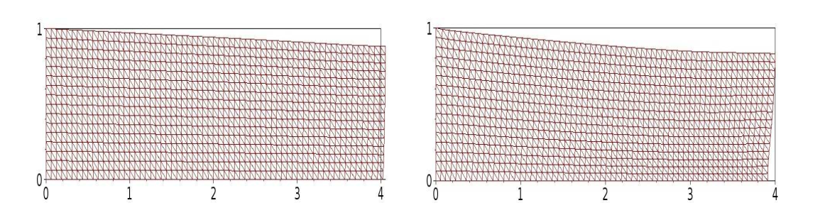
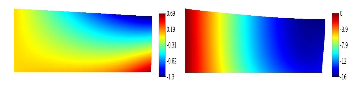
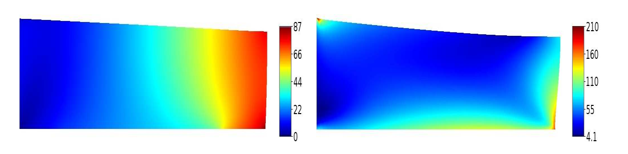
Here, we use as material the thermo-piezoelectric body whose constants are taken as [2]. The following data have been used in the numerical simulations:

\begin{eqnarray*} && r=10^{7}\, N /m^2 ,\;\; \mu = 0.2,\;\; \bar{k}_c= 1,\;\; \theta_f = 393 \,K,\;\; \theta_{ref} = 293 \,K.\\ && T= 10\, s,\;\; \mathbf{u}_0= \mathbf{0} \, m,\;\; \mathbf{v}_0= \mathbf{0} \, m/s,\;\; \varphi_0= 0 \, V,\;\; \theta_0= 0 \, K. \end{eqnarray*}

Our interest in this example is to study the influence of the thermal conductivity of the foundation on the contact process and, to this end, we consider the problem both in the case when the foundation is insulated there are no heat flux on \(\Gamma_C\) (i.e. \( \mathbf{q}\cdot \nu = 0\mbox{ on } \Gamma_C\)) and in the case when it is thermally conductive.

Figure 2 presents the deformed configurations for the two previously mentioned cases, at final time. We can easily note that considering a thermally conductive foundation reduce the deformations. In order to highlight the influence of the foundation temperature on the electric potential, we plot the electric potential for the two previously mentioned cases (see Figure 3). The first case illustrates the direct piezoelectric effect: the electric potential is generated because of the deformation. However, in the second case, we can easily note that considering a thermally conductive foundation increases the electric potential.

In Figure 4, the Von Mises stress norm is plotted on the deformed configuration. Clearly, effects due to the influence of foundation temperature, can be observed. Both temperature is plotted in Figure 5 at final time for the value \(\theta_f = 393\, K\).

5. Conclusion

In this paper thermo-piezoelectric contact including frictional heat generation and interfacial heat transfer is numerically studied. The novelties arise in the fact that the process is dynamic, the material behavior is described by a thermo-electro-elastic constitutive law and the foundation is thermally conductive. A fully discrete scheme was used to approach the problem and a numerical algorithm which combine the augmented Lagrangian approach with the Newton method was implemented. Moreover, numerical simulations for a representative two-dimensional example were provided. These simulations describe the thermal effect, i.e. the appearance of strain and voltage in the body, due to the action of the temperature field. Also, they underline the effects of the thermal contact, i.e. heat transfer and frictional heating, on the process. Performing these simulations, we found that the numerical solution worked well and the convergence was rapid. This work opens the way to study further models of frictional contact with a coefficient of friction depending on the slip rate or the temperature.

Conflicts of Interest

''The author declares no conflict of interest.''