
The main aim of fluid mechanics, as a multiform phenomenon, is to perform modelling of the liquids and gases in their common temperature and pressure ranges. Conservation of mass, momentum and energy can be taken as three basic laws for any engineering problem involving in the boundary layer theory. Recently, the complexity of such problems can be greatly simplified by using the approximate solution methodologies. In this way, Raees et al. [1] proposed a multiple solution for homogeneous-heterogeneous reactions on the Oberbeck-Boussinesq buoyancy-driven flow of dilute nanofluids. They derived the governing nonlinear equations based on the Buongiorno’s mathematical model, and showed that the dilute nanofluid gives a higher stability of chemical reactions than a typical one. Ghiasi and Saleh [2] analyzed the Casson type fluid over an unsteady shrinking surface in the presence of Joule heating and magnetic inclination. They showed that the effect of viscous force in their model will be usually negligible for large values of the Hartmann number. Gaffar et al. [3] employed the Keller box finite difference method (FDM) to simulate the thermomechanical behaviour of viscoelastic Jeffery’s fluid inside a non-parallel vertical channel so that an excellent consistency with those of Hossain and Paul [4] was captured. They also proved that the predicted behaviour is quite elastic with large Deborah numbers. Sayyed et al. [5] took the influence of permeability and slip boundary condition into account to study the geothermal aspects of flow over a wedge-shaped configuration. They combined the differential transformation method (DTM) with the Padé approximation, and showed that the suction in this case has the same effect as the injection on the permeability. Besthapu et al. [6] extended the double stratification (i.e., the stratified medium due to the temperature and nanoparticle concentration fields) to the laminar boundary layer flow along an exponentially stretching surface, which previously was reported by Khan and Pop [7]. Furthermore, they showed that their results are in good agreement with those obtained by Ishak [8].
Melting heat transfer can be briefly defined as follows: The melt liquid has not been diffused into the ambient liquid [9,10]. It has found many applications in engineering and physics, for example, to magma solidification, to semiconductor materials, thawing permafrost, etc. However, as we will now see, there exist only a few research studies concerning this issue. Hayat et al. [11] performed a melting heat transfer analysis of Powell-Eyring fluid with convective boundary conditions. Sheikholeslami and Rokni [12] used a similar idea applied to the forced convection flows considering the Buongiorno’s mathematical model. They showed that the drag force distribution generated from the magnetic field affects the momentum boundary layer thickness. Valipour et al. [13] investigated the heat and mass transfer characteristics of two-phase nanofluids induced by nonlinearly rotating plates carried out numerically in the standard MAPLE software. They found that the rotational velocity and temperature distributions enhance with an increase in the Reynolds number. Hayat et al. [14] employed the perturbation technique to analyze the melting heat transfer of peristaltic flows in the presence of viscous dissipation and Joule heating. They also analyzed the oscillatory heat transfer caused by the sinusoidal traveling wave in a channel.
It is noteworthy to mention that although some sort of solution methodologies has been employed to investigate the melting heat transfer characteristics to date [15-26], the homotopy-based methodology, due to its optimization performed in MATHEMATICA package BVPh2.0 [27], can be developed as an efficient procedure compared to any other one [11,28]. It is found that this methodology does not suffer from long run-time and can provide high accuracy estimates. The rest of the paper is organized as follows: Section 2 deals exclusively with the mathematical formulation. Section 3 outlines the homotopy-based methodology and its optimization. Section 4 focuses on the results and discussion. The concluding remarks are summarized in Section 5.
Let us denote the constitutive equation for an isotropic and incompressible flow of Casson fluid as follows [29]:
\[\begin{aligned} \label{eq1} \tau_{ij} = \begin{cases} 2 \bigg(\mu_{B}) + \frac{p_{y}}{\sqrt{2 \pi}} \bigg) e_{ij}, & \pi > \pi_{c}, \\ 2 \bigg( \mu_{B}) + \frac{p_{y}}{\sqrt{2 \pi_{c}}} \bigg) e_{ij}, & \pi > \pi_{c}, \\ \end{cases} \end{aligned} \tag{1}\] where \(\tau_{ij}\) is the Cauchy stress tensor, \(\mu_{B}\) is the plastic dynamic viscosity, \(p_{y} \bigg( = \frac{\mu_{B} \sqrt{2 \pi}}{\lambda} \bigg)\) is the fluid yield stress, \(e_{ij}\) is the \((i,j)th\) component(s) of the deformation rate, \(\pi ( =e_{ij} e_{ij})\) is the product of the deformation rate component(s), \(\pi_{c}\) is the critical value of \(\pi\) and \(\lambda\) is termed as the Casson fluid parameter. In the case of \(\pi > \pi_{c}\), Equation (1) reduces to [30],
\[\begin{aligned} \label{eq2} \mu_{nf} = \mu_{B} + \frac{p_{y}}{\sqrt{2 \pi}} = \mu_{B} \bigg( 1 + \frac{1}{\lambda} \bigg), \end{aligned} \tag{2}\] where \(\mu_{nf}\) is the dynamic viscosity. According to the above formula, the kinematic viscosity can be defined as \[\begin{aligned} \label{eq3} v_{nf} = \frac{\mu_{B}}{\rho_{nf}} \bigg( 1 + \frac{1}{\lambda} \bigg), \end{aligned} \tag{3}\] where \(\rho_{nf}\) is the density.
The velocity and temperature fields for a two-dimensional laminar flow in the Cartesian coordinates take the form
\[\begin{aligned} \label{eq4} \mathbb{V} = [ u(x,y), v(x,y)], \ \ \mathbb{T} = T(x,y) \end{aligned} \tag{4}\] where \(u\) and \(v\) are the velocity components along the \(x\) and \(y\) directions, respectively, and \(T\) is the temperature.
By eliminating the pressure terms, one can obtain a set of governing PDEs in the following form
\[\begin{aligned} \label{eq5} \begin{cases} \displaystyle \frac{\partial u}{\partial x} + \frac{\partial v}{\partial y} = 0, \\ \displaystyle u \frac{\partial x}{\partial x} + v \frac{\partial u}{\partial y} = v_{nf} \bigg( 1 + \frac{1}{\lambda} \bigg) \frac{\partial^2 u} {\partial y^2}, \\ \displaystyle (\rho c_{p})_{nf} \bigg( u \frac{\partial T}{\partial x} + v \frac{\partial T}{\partial y} \bigg) = k_{nf} \frac{\partial ^2 T}{\partial y^2} – \frac{\partial q_{r}}{\partial y} \end{cases} \end{aligned} \tag{5}\] with the boundary conditions \[\begin{aligned} \label{eq6} \begin{cases} \displaystyle u = U_{w} = ax, \ \ T = T_{m}, & at \ y = 0, \\ \displaystyle u \rightarrow 0, T \rightarrow T_{\infty}, & as \ y \rightarrow \infty, \end{cases} \end{aligned} \tag{6}\] and [10],
\[\begin{aligned} \label{eq7} \displaystyle k_{nf} (\frac{\partial T }{\partial y })_{y = 0} = \rho_{nf} [\delta + c_{s}(T_{m} – T_{0}) v(x, 0), \end{aligned} \tag{7}\] where \(c_{p}\) is the specific heat at constant pressure, \(k_{nf}\) is the thermal conductivity, \(q_{r}\) is the radiation heat flux, \(U_{w}\) is the velocity at the wall, \(a > 0\) is an arbitrary constant, \(T_{m}\) is the temperature of the melting surface, \(T_{\infty}\) is the ambient temperature, \(\delta\) is the latent heat of the fluid, \(c_{s}\) is the heat capacity of the solid surface and \(T_{0}\) is the temperature of the solid surface. According to the basic hypothesis of Rosseland approximation [31], the radiation heat flux presented in Equation (5) becomes
\[\begin{aligned} \label{eq8} q_{r} = -\frac{4 \sigma^*}{3k^*} \frac{\partial T^4}{\partial y}, \end{aligned} \tag{8}\] where \(\sigma^*\) and \(k^*\) are the Stefan-Boltzmann constant and the mean absorption coefficient, respectively. Assuming that the fluid-phase temperature discrepancy within the flow is sufficiently small [32], \(T^4\) can be expanded in the Taylor series as follows
\[\begin{aligned} \label{eq9} T^4 = T^4_{\infty} + 4T^3_{\infty}(T – T_{\infty}) + 6 T^2_{\infty} (T – T_{\infty})^2 + \dots \cong 4T^3_{\infty} T – 3T^4_{\infty}. \end{aligned} \tag{9}\]
By substituting Equation (9) into Equation (8), one would get
\[\begin{aligned} \label{eq10} q_{r} = – \frac{16 \sigma^* T^3_{\infty}}{3k^*} \frac{\partial T}{\partial y}, \end{aligned} \tag{10}\]
The similarity variables, which convert Equation (5) into the ODEs are given by \[\begin{aligned} \label{eq11} \displaystyle \eta = y \sqrt{\frac{a}{v_{nf}}}, \ \ \psi = \sqrt{a v_{nf} } x f(\eta), \ \ \theta(\eta) = \frac{T – T_{m}}{T_{\infty} – T_{m}}, \end{aligned} \tag{11}\] where \(\eta\) is the similarity parameter, \(\psi\) is the stream function which satisfies the continuity equation (i.e. \(u= \frac{\partial \psi}{\partial y}\) and \(v = – \frac{\partial \psi}{\partial x})\), \(f\) is the similarity function and \(\theta\) is the dimensionless temperature.
By substituting Equations (10) and (11) into Equation (5), the following set of governing ODEs can be expressed as \[\begin{aligned} \label{eq12} \begin{cases} \displaystyle \bigg( 1 + \frac{1}{\lambda} \bigg) \frac{\partial^3 f}{\partial \eta^3} + f \frac{\partial^2 f}{\partial \eta^2} – \bigg( \frac{\partial f}{\partial \eta} \bigg)^2 = 0,\\ \displaystyle \frac{1}{Pr} \bigg( 1 + \frac{4}{3} N \bigg) \frac{\partial^2 \theta}{\partial \eta^2} + f \frac{\partial \theta}{\partial \eta} = 0, \end{cases} \end{aligned} \tag{12}\] with the boundary conditions
\[\begin{aligned} \label{eq13} \begin{cases} \displaystyle \frac{\partial f}{\partial \eta} = 1, \ \ Prf + \beta \frac{\partial \theta}{\partial \eta} = 0, \ \ \theta = 0, & at \ \eta = 0, \\ \displaystyle \frac{\partial f}{\partial \eta} = 0, \ \ \theta = 1, & as \ \eta \rightarrow \infty, \end{cases} \end{aligned} \tag{13}\] where \(\Pr = \frac{\mu_{nf} c_{p}}{k_{nf}}\) is the Prandtl number, \(N = \frac{4 \sigma^* T^3_{\infty}}{k_{nf} k^*}\) is the radiation parameter and \(\beta = \frac{c_{p} (T_{\infty} – T_{m} )}{ \delta + c_{s} (T_{m} – T_{0}) }\) is the melting parameter.
Here, the physical quantities of interest i.e., the skin friction coefficient and local Nusselt number can be defined as,
\[\begin{aligned} \label{eq14} C_{f} = \frac{\tau_{w}}{\rho_{nf} U^2_{w} }, \ \ Nu_{x} = \frac{x q_{w}}{k_{nf} (T_{\infty } – T_{m})}, \end{aligned} \tag{14}\] where \[\begin{aligned} \label{eq15} \tau_{w} = \mu_{nf} \bigg( \frac{\partial u}{\partial y} \bigg)_{y = 0} , \ \ q_{w} = -k_{nf} \bigg( \frac{\partial T}{\partial y} \bigg)_{y = 0}, \end{aligned} \tag{15}\]
By substituting Equation (11) into Equations (14) and (15) we see that
\[\begin{aligned} \label{eq16} Re^{1/2}_{x} C_{f} = \bigg( 1 + \frac{1}{\lambda} \bigg) \bigg( \frac{\partial^2 f}{\partial \eta^2} \bigg)_{\eta = 0}, \ \ Re^{-1/2}_{x} Nu_{x} = – \bigg( \frac{\partial \theta}{\partial \eta} \bigg)_{\eta = 0}, \end{aligned} \tag{16}\] where \(Re_{x} = \frac{x U_{w}}{v_{nf}}\) is the local Reynolds number.
As it was mentioned earlier, finding an exact closed-form solution for the third-order nonlinear ODEs given in Equation (12) is not generally possible. According to the basic concept of homotopy-based methodology, the governing ODEs should be discretized to an infinite sequence of linear functions employing a typical series expansion such as Taylor, Maclaurin, etc. [33,34]. It is worth mentioning that choosing an appropriate auxiliary parameter provides a convenient way to adjust the convergence of series solution [33,35]. Furthermore, unlike perturbation techniques, this methodology can be applied to any type of ODEs and associated boundary conditions consisting of small or large parameters [36]. In this way, we choose the initial guesses and auxiliary linear operators as follows,
\[\begin{aligned} \label{eq17} f_{0} = 1 – e^{-\eta} – \frac{\beta}{Pr}, \ \ \theta_{0} = 1 – e^{-\eta}, \end{aligned} \tag{17}\]
\[\begin{aligned} \label{eq18} \textbf{L}_{f} = \frac{\partial^3 f}{\partial \eta^3 } – \frac{\partial f}{\partial \eta}, \ \ \textbf{L}_{\theta} = \frac{\partial^2 \theta}{\partial \eta^2} – \theta, \end{aligned} \tag{18}\] with the properties \[\begin{aligned} \label{eq19} \textbf{L}_{f} [C_{1} + C_{2} e^\eta + C_{3} e^{-\eta} ] = 0, \ \ \textbf{L}_{\theta } [ C_{4} e^\eta + C_5 e^{-\eta} ] = 0, \end{aligned} \tag{19}\] where \(C_1 -C_5\) are the integration constants. By introducing \(q \in [0 ,1 ]\) as an embedding parameter, the zeroth order deformation equations are constructed as [33],
\[\begin{aligned} \label{eq20} \begin{cases} (1 – q) \textbf{L}_f [\bar{f} (\eta; q) – f_0 (\eta)] = q \hslash_f \textbf{N}_f [\bar{f} (\eta;q)], \\ (1 – q) \textbf{L}_\theta [\bar{\theta} (\eta; q) – \theta_0 (\eta)] = q \hslash_f \textbf{N}_\theta [\bar{f} (\eta;q), \bar{\theta} (\eta;q)], \\ \end{cases} \end{aligned} \tag{20}\] where \(\hslash_f\) and \(\hslash_\theta\) are the so-called auxiliary parameters, and \(\textbf{N}_f\) and \(\textbf{N}_\theta\) are the nonlinear differential operators which can be expressed as follows,
\[\begin{aligned} \label{eq21} \begin{cases} \textbf{N}_f[\bar{f}(\eta; q)] = \bigg( 1+ \frac{1}{\lambda} \bigg) \frac{\partial^3 \bar{f} (\eta; q)}{\partial \eta^3} + \bar{f} (\eta; q) \frac{\partial^2 \bar{f} (\eta; q)}{\partial \eta^2} – \bigg( \frac{\partial \bar{f} (\eta; q)}{\partial \eta} \bigg)^2 , \\ \textbf{N}_\theta [\hat{f}(\eta; q), \bar{\theta} (\eta; q)] = \frac{1}{Pr} \bigg( 1+ \frac{4}{3}N \bigg) \frac{\partial^2 \bar{\theta} (\eta; q)}{\partial \eta^2} + \bar{f} (\eta; q) \frac{\partial \bar{\theta} (\eta; q)}{\partial \eta} , \\ \end{cases} \end{aligned} \tag{21}\] with the boundary conditions,
\[\begin{aligned} \label{eq22} \begin{cases} \displaystyle \frac{\partial \bar{f} (\eta ; q)}{\partial \eta} = 1, \ \ Pr \bar{f} (\eta ; q) + \beta \frac{\partial \bar{\theta}(\eta; q)}{\partial \eta} = 0, \ \ \bar{\theta} (\eta ; q) = 0, & at \ \eta = 0, \\ \displaystyle \frac{\partial \bar{f} (\eta ; q)}{\partial \eta} = 0, \ \ \bar{\theta} (\eta; q) = 1, & as \ \eta \rightarrow \infty, \end{cases} \end{aligned} \tag{22}\]
As \(q\) increases from \(0\) to \(1\), \(\bar{f}̅(\eta;q)\) and \(\bar{\theta} ̅(\eta;q)\) vary from the initial guesses \(f_0 (\eta)\) and \(\theta_0 (\eta)\) to the exact solutions \(f(\eta)\) and \(\theta(\eta)\), respectively. Expanding \(\bar{f} ̅(\eta;q)\) and \(\bar{\theta} ̅(\eta;q)\) in the Taylor series with respect to \(q\) gives,
\[\begin{aligned} \label{eq23} \bar{f} (\eta ; q ) = \bar{f} (\eta ; 0) + \sum_{n = 1}^{\infty} f_n (\eta)q^n, \ \ \bar{\theta} (\eta; q) = \bar{\theta} (\eta; 0) +\sum_{n = 1}^{\infty} \theta_n (\eta) q^n, \end{aligned} \tag{23}\] where \(f_n\) and \(\theta_n\) are the nth-order deformation derivatives, that is,
\[\begin{aligned} \label{eq24} f_n(\eta ) = \bigg( \frac{1}{n!} \frac{\partial^n \bar{f} (\eta; q)}{\partial q^n} \bigg)_{q = 0}, \ \ \theta_n(\eta) = \bigg( \frac{1}{n!} \frac{\partial^n \bar{\theta} (\eta; q)}{\partial q^n} \bigg)_{q = 0}, \end{aligned} \tag{24}\]
It is to be noted here that the solution of Equation (20) depends only on the auxiliary linear operators, initial guesses and auxiliary parameters [33]. Accordingly, if these quantities are properly selected so the series Equation (23) converges at \(q=1\) in the following form \[\begin{aligned} \label{eq25} f(\eta ) = \sum_{n = 0}^{\infty } f_n (\eta) , \ \ \theta (\eta ) = \sum_{n = 0}^{\infty } \theta_n (\eta), \end{aligned} \tag{25}\]
By Differentiating Equation (20) \(n\) times with respect to \(q\), then setting \(q=0\) and dividing them by \(n!\), one can obtain the nth-order deformation equations as follows \[\begin{aligned} \label{eq26} \textbf{L}_f[f_n(\eta) – \chi_n f_{n-1} (\eta) ] = \hslash \textbf{R}_{f,n}(\eta ) , \ \ \textbf{L}_{\theta} [ \theta_n (\eta) – \chi_n \theta_{n-1} (\eta) ] = \hslash_\theta \textbf{R} _{\theta, n} (\eta), \end{aligned} \tag{26}\] where \[\begin{aligned} \label{eq27} \chi_n = \begin{cases} 0, & n \leq 1, \\ 1, & n \ge 1, \end{cases} \end{aligned} \tag{27}\]
\[\begin{aligned} \label{eq28} \begin{cases} \textbf{R}_{f,n } (\eta) = \bigg( 1 + \frac{1}{\lambda} \bigg) \frac{\partial^3 f_{n-1}}{\partial \eta^3} + \sum_{m = 0}^{m -1} f_m \frac{\partial^2 f_{n-m-1}}{\partial \eta^2} – \sum_{m = 0}^{n – 1} \frac{\partial f_m}{\partial \eta} \frac{\partial f_{n – m – 1}}{\partial \eta}, \\ \textbf{R}_{\theta , n} (\eta ) = \frac{1}{Pr} \bigg( 1 + \frac{4}{3} N \bigg) \frac{\partial^2 \theta_{n-1}}{\partial \eta^2} + \sum_{m = 0}^{m – 1} f_m \frac{\partial \theta_{n-m- 1}}{\partial \eta}. \end{cases} \end{aligned} \tag{28}\]
To complete the solution procedure, it is sufficient to set the given boundary conditions given in Equation (22) equal to zero, obtain the arbitrary constants \(C_1-C_5\), and thereby derive the general solutions of Equation (26) as
\[\begin{aligned} \label{eq29} \begin{cases} f_n (\eta ) = f^*_n (\eta ) – \bigg[ f^*_n (0) + \frac{\partial f^*_n(0)}{\partial \eta} (1 – e^{-\eta}) \bigg] – \frac{\beta}{Pr} \bigg( \theta^*_n (0) + \frac{\partial \theta^*_n (0)}{\partial \eta} \bigg), \\ \theta_n(\eta ) = \theta^*_n (\eta) – \theta^*_n(0)e^{- \eta}, \end{cases} \end{aligned} \tag{29}\] where \(f_n^* (\eta)\) and \(\theta_n^* (\eta)\) are the particular solutions. Hence, after solving the nth-order deformation Equation (26), the \(nth-\)order approximate solutions are given by
\[\begin{aligned} \label{eq30} f_p(\eta) = \sum_{ n = 0}^{p} f_n (\eta ), \ \ \theta_n (\eta) = \sum_{ n = 0}^{p} \theta_n (\eta), \end{aligned} \tag{30}\]
Here, in the context of optimization, the following squared residual errors are defined as [37],
\[\begin{aligned} \label{eq31} \begin{cases} \varepsilon_{f, p } = \frac{1}{ j + 1} \sum_{i =0}^{j} \bigg( \textbf{N}_f [ \sum_{r = 0}^{p} f(\eta) ]_{\eta = i \delta \eta} \bigg)^2 \delta \eta, \\ \varepsilon_{\theta, p} = \frac{1 }{j + 1} \sum_{i =0}^{j} \bigg( \textbf{N}_\theta [ \sum_{r = 0}^{p} f(\eta), \ \sum_{r = 0}^{p} \theta (\eta)]_{\eta = i \delta \eta} \bigg)^2 \delta \eta, \end{cases} \end{aligned} \tag{31}\] where \(j=20\) and \(\delta \eta = 0.5\) [38,39].
To find the optimal values of auxiliary parameters and number of iterations, a convergence study performed in MATHEMATICA package BVPh2.0 [27] is provided here. To this end, the governing physical parameters involved in Equations (12) and (13) are given in Table 1. According to the results of Table 2, the optimal values of auxiliary parameters decrease when the order of approximation is increased. Hence, in what follows, only \(\hslash_f= -0.64492\) and \(\hslash_\theta=-0.85516\) are employed to ensure the high accuracy estimates. Furthermore, Table 3 represents the values of squared residual errors at different orders. It is observed form this table that the series solution will thoroughly be converged if the number of iterations is set equal to \(p=20\).
| \(\lambda\) | \(Pr\) | \(N\) | \(\beta\) |
| 0.5 | 6.2 | 0.1 | 0.4 |
| \(n=1\) | \(n=2\) | \(n=3\) | \(n=4\) | \(n=5\) | |
| \(\hslash_f\) | -0.49304 | -0.55176 | -0.59709 | -0.62530 | -0.64492 |
| \(\hslash_\theta\) | -0.72170 | -0.76209 | -0.79720 | -0.82814 | -0.85516 |
| \(p\) | \(\varepsilon_f,p\) | \(\varepsilon_\theta,p\) |
| 2 | \(4.119 \times 10^-6\) | \(2.071 \times × 10^-7\) |
| 4 | \(2.169 \times 10^-7\) | \(7.195 \times 10^-8\) |
| 6 | \(8.403 \times 10^-8\) | \(3.040 \times 10^-8\) |
| 8 | \(5.125 \times 10^-8\) | \(8.955 \times 10^-9\) |
| 10 | \(1.108 \times 10^-8\) | \(5.011 \times 10^-9\) |
| 12 | \(8.925 \times 10^-9\) | \(2.322 \times 10^-9\) |
| 14 | \(6.881 \times 10^-9\) | \(9.170 \times 10^-10\) |
| 16 | \(3.230 \times 10^-9\) | \(6.989 \times 10^-10\) |
| 18 | \(1.014 \times 10^-9\) | \(4.721 \times 10^-10\) |
| 20 | \(9.175 \times 10^-10\) | \(1.990 \times 10^-10\) |
| \(\beta= 0.3\) | \(\beta=0.6\) | \(\beta=1\) | \(\beta= 1.5\) | \(\beta=2\) | |
| BVPh2.0 | 1.70863 | 1.66414 | 1.63186 | 1.60748 | 1.59119 |
| Krishnamurthy et al. | 1.70978 | 1.66571 | 1.63308 | 1.60870 | 1.59262 |
As it can be seen from Table 4, increasing the value of melting parameter decreases the skin friction coefficient. This is due to the fact that by increasing the melting parameter, a temperature discrepancy between the solid and melting surfaces generates which is led to the molecular motion of the particles. Furthermore, Table 4 provides a comparison between the present findings and those reported by Krishnamurthy et al. [15]. Based on the results shown in this table, the present findings agree well with those of Krishnamurthy et al. [15] in all cases; because the relative error between them does not exceed 0.08%.
| \(Pr=0.07\) | \(Pr=0.2\) | \(Pr=0.7\) | \(Pr=2\) | \(Pr=7\) | |
| BVPh2.0 (\(\beta = 0\)) | 0.06629 | 0.16914 | 0.45386 | 0.91133 | 1.89532 |
| BVPh2.0 (\(\beta=1\)) | 0.05948 | 0.14201 | 0.41365 | 0.85961 | 1.49830 |
| BVPh2.0 (\(\beta = 2\)) | 0.04608 | 0.11872 | 0.37197 | 0.79193 | 1.21666 |
| BVPh2.0 (\(\beta= 3 \)) | 0.03915 | 0.09516 | 0.32557 | 0.73454 | 1.00410 |
| Khan and Pop | 0.0663 | 0.1691 | 0.4539 | 0.9113 | 1.8954 |
Table 5 investigates the variation of heat transfer rate versus the Prandtl number for some different melting parameters. According to this table, the heat transfer rate increases monotonically as the Prandtl number is increased from 0.07 to 7. This is because of the correspondence between the thermal conductivity and diffused heat energy [40]. In addition, as it can be observed from Table 5, the heat transfer rate decreases as the melting parameter increases which is only due to the existing energy dissipation. However, at very small melting parameters there is a low-temperature enhancement [19].
It is to be mentioned here that the accuracy of the present findings without its melting effect is verified by comparison with the numerical observations reported by Khan and Pop [7]. Hence, in view of the results listed in Tables 4 and 5, one can emphasize that employing the homotopy-based methodology and its optimization is sufficient to accelerate the convergence on any large interval and thereby ensure the accuracy and efficiency of the series solution. Here, for the sake of brevity, only the velocity and temperature distributions with and without the melting effect are provided in Table 6.
| \(\eta\) | \(\beta = 0 \) | \(\beta= 1 \) | ||
| \(\frac{\partial f(\eta)}{\partial \eta}\) | \(\theta (\eta)\) | \(\frac{\partial f(\eta)}{\partial \eta}\) | \(\theta (\eta)\P\) | |
| 0 | 1 | 0 | 1 | 0 |
| 0.1 | 0.9648 | 0.1459 | 0.9715 | 0.0865 |
| 0.2 | 0.9125 | 0.3040 | 0.9247 | 0.2095 |
| 0.3 | 0.7320 | 0.3619 | 0.7359 | 0.2470 |
| 0.4 | 0.5269 | 0.4495 | 0.5411 | 0.2773 |
| 0.5 | 0.4132 | 0.5137 | 0.4379 | 0.3406 |
| 0.6 | 0.3527 | 0.5715 | 0.3691 | 0.3812 |
| 0.7 | 0.3009 | 0.6630 | 0.3126 | 0.4391 |
| 0.8 | 0.2651 | 0.7002 | 0.2714 | 0.4980 |
| 0.9 | 0.2245 | 0.7356 | 0.2299 | 0.5719 |
| 1 | 0.0471 | 0.9354 | 0.0495 | 0.8147 |
| 2 | 0.0017 | 0.9836 | 0.0029 | 0.9441 |
| 3 | 0.0006 | 0.9915 | 0.0010 | 0.9790 |
| 4 | 0 | 1 | 0.0004 | 0.9899 |
| 5 | 0 | 1 | 0 | 0.9979 |
| 6 | 0 | 1 | 0 | 1 |
As it was mentioned in Section 2, the fluid yielding behavior is greatly affected by the shear and thermal history. Furthermore, the Casson fluid parameter plays a crucial role in the fluid yielding threshold of such rheological systems [41]. The reason is that the ratio of viscous force to yield stress increases with an increase in the Casson fluid parameter. It is worth noting that this increase of the Casson fluid parameter leads to the free flow movement with a specific pressure gradient. This issue is clearly illustrated in Figure 1.
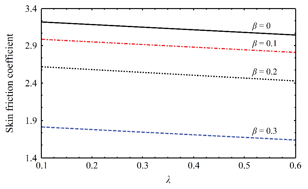
According to Figure 1, one can observe that the skin friction coefficient decreases with an increase in the Casson fluid parameter; however, Mabood et al. [22] have provided some evidence to illustrate that this coefficient in some cases is relatively insensitive to the Casson fluid parameter. The discrepancy between the present paper and that reported by Mabood et al. [22] is due to the presence of temperature-dependent dynamic viscosity and its roughly exponential function.
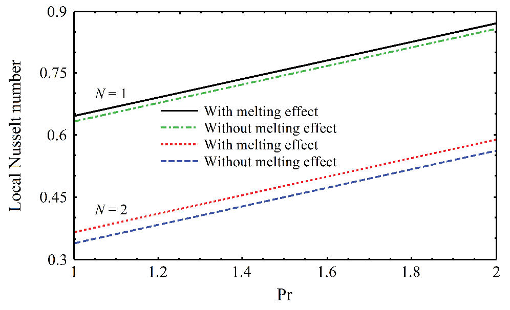
Based on the results presented in Figure 2, neglecting the melting effect decreases slightly the local Nusselt number. Furthermore, increasing the value of radiation parameter decreases the effect of melting on increasing the local Nusselt number. It is due to a reduction in the mean absorption coefficient and consequently divergence of the radiation heat flux. Thus, it is desirable to consider this observation in some cases as the basis of controlling the thermal radiation from solid and melting surfaces.
The present paper aimed to provide an investigation of how the melting effect can be applied to a set of governing PDEs which govern a two-dimensional laminar flow of Casson fluid. In this way, the conservation of mass, momentum and energy, combined with the Rosseland approximation, were employed and reduced to a system of ODEs through the similarity variables. The homotopy-based methodology performed in MATHEMATICA package BVPh2.0 was developed because the series solution to be optimized depends significantly on choosing the appropriate auxiliary parameters. The accuracy of the present findings was also verified by comparison with the numerical results in the literature. Since the author’s perspective was to introduce the idea of melting effect, the main inferences in this case can be summarized as follows:
In general, the velocity and temperature distributions are affected by the melting parameter more than that of the other pertinent parameters.
Accounting for the effect of Casson fluid as well as increasing the melting parameter decreases the skin friction coefficient.
Accounting for the effect of thermal conductivity as well as increasing the melting parameter decreases the heat transfer rate.
Accounting for the effect of thermal radiation as well as increasing the melting parameter increases the local Nusselt number.
\(p_y\): fluid yield stress
\(e_{ij}\): \((i,j)th\) component(s) of the deformation rate
\(\mathbb{V}\): velocity field
\(u and v\): velocity components along the \(x\) and \(y\) directions, respectively
\(\mathbb{T}\): temperature field
\(T\): temperature
\(c_p\): specific heat at constant pressure
\(k_{nf}\): thermal conductivity
\(q_r\): radiation heat flux
\(U_w\): velocity at the wall
\(T_m\): temperature of the melting surface
\(T_\infty\): ambient temperature
\(c_s\): heat capacity of the solid surface
\(T_\theta\): temperature of the solid surface
\(k^*\): mean absorption coefficient
\(f\): similarity function
\(Pr\) : Prandtl number
\(N\): radiation parameter
\(Re_x\): local Reynolds number
Greek symbols
\(τ_{ij}\): Cauchy stress tensor
\(μ_B\): plastic dynamic viscosity
\(\pi\): product of the deformation rate component(s)
\(\pi_c\): critical value of \(\pi\)
\(\lambda\): Casson fluid parameter
\(μ_{nf}\): dynamic viscosity
\(υ_{nf}\): kinematic viscosity
\(\rho_{nf}\): density
\(\alpha\): arbitrary constant
\(\delta\): latent heat of the fluid
\(\sigma^*\): Stefan-Boltzmann constant
\(\eta\): similarity parameter
\(\psi\): stream function
\(\theta\): dimensionless temperature
\(\beta\): melting parameter
Subscripts
\(ij\): tensor index
\(c\): critical
\(nf\): nanofluid
\(r\): radiation
\(w\): condition at the wall
\(m\): melting
\(\infty\): condition at the ambient medium
\(s\): solid