Contact problems are everywhere in mechanics, physics, and engineering applications. Some examples from the automotive industry are the contact between brake pads and rotors or between pistons and cylinders. Thermal effects in contact processes affect the composition and stiffness of the contacting surfaces and cause thermal stresses in the contacting bodies (see [1]). Vice versa, the current temperature may influence the elastic material response. In the literature, it is possible to find different works which studied and developed different thermomechanical frictional problems, such as [1-5] and the references therein. There, besides the rigorous construction of various mathematical models of contact with thermal effects, the unique weak solvability of these models was proved by using arguments of variational and hemivariational inequalities. Moreover, other works in the literature, such as [6-12] present a numerical solution for frictional contact problems by considering the thermal effects.
Recently, a new frictionless contact model for thermoelastic materials has been studied theoretically in [13]. In this model, there are two unilateral constraint sets; one is needed for the normal displacement in the Signorini condition on the part of the boundary, while the other one for the temperature provides a unilateral obstacle for the temperature inside a domain. The contact is described with a thermal conductivity condition, in which the heat exchange coefficient is not a constant but a function of the normal displacement on the contact boundary. The current work represents a continuation of [13]. But, unlike [13], in this work, a frictionless contact problem between a thermoelastic body and a thermally conductive foundation is numerically studied, in which the heat exchange coefficient is a function of the contact pressure (see [6,7]). The numerical approach of this model represents the main trait of the novelty of the present paper. To this end, two contact algorithms based on the penalty and the augmented Lagrangian approaches are discussed and successfully applied to the modeling of this system. This work compares numerical solutions of the approximate thermal contact problem and the Lagrangian one.
The paper is organized as follows: Section 2 provides a brief description of the model and its variational formulation. In Section 3, we consider a numerical approximation of the model using the finite element method, while applying a penalty method to resolve the inequality constraints. Section 4 details the augmented Lagrangian-based approximation. In Section 5, we present numerical simulations that validate our approximation method, followed by a conclusion in Section 6.
First, we describe the physical setting of the contact problem. A thermoelastic body occupies an open bounded domain \(\Omega\subset\mathbb{R}^d\,\, (d=2,3)\) with a smooth boundary \(\partial \Omega=\Gamma\) and denote by \(\mathbf{\nu} = (\nu_i)\) its unit outward normal. The body forces of density \(\mathbf{f}_{0}\) is applied in \(\Omega\), and we assume that a heat source of constant strength \(q_0\) is present. The body is submitted to mechanical and thermal constraints on the boundary. To describe them, the boundary \(\Gamma\) is divided into three disjoint sets \(\Gamma_D\), \(\Gamma_N\) and \(\Gamma_C\). We assume that \(meas\,\Gamma_D>0\). The body is clamped on \(\Gamma_D\). The surface traction of density \(\mathbf{f}_N\) acts on \(\Gamma_N\). We suppose that the temperature vanishes in \(\Gamma_D\cup\Gamma_N\). Over the contact surface \(\Gamma_C\), the body comes in contact with a thermally conductive foundation. The contact is frictionless and modeled with Signorini’s conditions. Here and below, an index that follows a comma represents the partial derivative concerning the corresponding component of the spatial variable, i.e., \(f_{,i}=\frac{\partial f}{\partial x_i}\).
We denote by \(\mathbf{u} = (u_i) \in\mathbb{R}^d\) the displacement field, by \({\sigma}=(\sigma_{ij})\in \mathbb{S}^d\) the stress, by \(\mathbf{\varepsilon(u)}=(\varepsilon_{ij}(\mathbf{u}))\in \mathbb{S}^d\) the linearized strain tensor, \(\theta\in\mathbb{R}\) the temperature, and by \(\mathbf{q} = (q_i) \in\mathbb{R}^d\) the heat flux. Let \(\mathbb{S}^d\) be the space of second order symmetric tensors on \(\mathbb{R}^d\). The functions \(\mathbf{u}\in\mathbb{R}^d\), \({\sigma}\in\mathbb{S}^d\), \(\theta\in\mathbb{R}\) and \(\mathbf{q} \in\mathbb{R}^d\) are the unknowns of the problem. To describe the boundary conditions we use the usual notation \(u_\nu=\mathbf{u}\cdot \mathbf{nu}\), \(\sigma_\nu={\sigma}\mathbf{\nu}\cdot \mathbf{\nu}\) and \({\sigma}_\tau={\sigma}-\sigma_\nu\mathbf{\nu}\). We recall that the divergence operators for tensor and vector functions are defined by \(Div{\sigma}=(\sigma_{ij,j})\) and \(div\mathbf{q}=(q_{i,i})\), respectively.
We model the behavior of the material with a constitutive law of the form; \[\begin{array}{l} {\sigma} = {\mathcal{F}} {\varepsilon}(\mathbf{u}) – \mathcal{M}\theta \quad \hbox{in} \quad \Omega, \end{array}\] and the heat flux \(\mathbf{q}\) is given by the following Fourier-type law: \[\mathbf{q} =-\mathcal{K}\nabla\theta \quad \hbox{in} \quad \Omega\,,\] here \({\mathcal{F}}=(f_{ijkl})\), \(\mathcal{M}=(m_{ij})\) and \(\mathcal{K}=(k_{ij})\) are respectively, the elasticity, thermal expansion and thermal conductivity tensors.
We assume that the process is static, then the equations of stress equilibrium and the heat conduction equation are \[\begin{array}{l} {Div {\sigma}+ \mathbf{f}_{0}=\mathbf{0} \quad \hbox{in} \quad \Omega, }\\ { div \mathbf{q} =q_0\quad\quad \quad \hbox{in} \quad \Omega.} \end{array}\] The Dirichlet and Neumann boundary condition, respectively, are stated by \[\begin{array}{l} \mathbf{u}=\mathbf{0}\quad\quad\quad \;\hbox{on} \quad \Gamma_D,\\ {\sigma} \mathbf{u}=\mathbf{f}_N \quad\quad \hbox{on}\quad \Gamma_N. \end{array}\] Next, on \(\Gamma_D\cup \Gamma_N\) we prescribe a Dirichlet condition for the temperature, say, \[\theta=0 \quad \hbox{on} \quad \Gamma_D\cup\Gamma_N.\] We assume that the contact is frictionless and it is modeled with Signorini’s condition, that is \[u_\nu – g \leq 0,\quad \sigma_\nu\leq 0,\quad \sigma_\nu (u_\nu – g) =0,\quad {\sigma}_\tau=\mathbf{0}\quad \hbox{on} \quad \Gamma_C,\] where \(g\) is the gap between the body and the foundation.
Next, we describe the boundary condition for the temperature on \(\Gamma_C\). We assume that there is heat exchange between the surface and the foundation, which is at temperature \(\theta_f\). We assume a boundary condition of the following form \[\mathbf{q}\cdot \mathbf{u} = k_c (\sigma_\nu)\big(\theta – \theta_f\big) \quad \mbox{on} \quad\Gamma_C,\] where \(k_c(\cdot)\) is the normal pressure dependent heat exchange coefficient and has to satisfy \(k_c(0)=0\). This condition guarantees that there is no heat flux between the body and the foundation if they are not in contact. For \(k_c(\cdot)\), we employ a linear model \(k_c(\sigma_\nu) = \bar{k}_c|\sigma_\nu|\), where \(\bar{k}_c\geq 0\) is model constant, see [6,7].
Finally, to guarantee the durable years of the material, we suppose that the temperature \(\theta\) in the domain \(\Omega\) satisfies the obstacle condition: \[\theta\leq \theta_0\quad\mbox{in}\quad\Omega,\] where the temperature \(\theta_0\) is assumed to be known, see [13].
Under these conditions, our mechanical problem may be formulated as follows.
Problem 1. Find a displacement field \(\mathbf{u}:\Omega\to\mathbb{R}^d\), a stress field \({\sigma}:\Omega\to\mathbb{S}^d\), a temperature \(\theta:\Omega\rightarrow \mathbb{R}\), and a heat flux \(\mathbf{q}:\Omega\to\mathbb{R}^d\) such that \[ {\sigma}=\mathcal{F}{\varepsilon}(\mathbf{u}) – \mathcal{M}\theta \qquad \qquad \qquad \hbox{in} \quad \Omega, \tag{1}\]\[ \mathbf{q} =-\mathcal{K}\nabla\theta \qquad \qquad \qquad \hbox{in} \quad \Omega, \tag{2}\]\[ Div {\sigma}+ \mathbf{f}_0=\mathbf{0} \qquad \qquad \qquad \hbox{in} \quad \Omega, \tag{3}\]\[ div \mathbf{q} =q_0 \qquad \qquad \qquad \hbox{in} \quad \Omega, \tag{4}\]\[ \mathbf{u}=\mathbf{0}\qquad \qquad \qquad \hbox{on} \quad \Gamma_D, \tag{5}\]\[ {\sigma} \mathbf{u}=\mathbf{f}_N \qquad \qquad \qquad \hbox{on}\quad \Gamma_N, \tag{6}\]\[ u_\nu – g \leq 0,\quad\sigma_{\nu}\leq 0,\quad \sigma_\nu (u_\nu – g ) =0 \qquad \qquad \qquad\hbox{on}\quad \Gamma_C, \tag{7}\]\[ {\sigma}_{\tau} = \mathbf{0} \qquad \qquad \qquad \hbox{on}\quad \Gamma_C, \tag{8}\]\[\theta=0 \qquad \qquad \qquad \hbox{on} \quad \Gamma_D\cup\Gamma_N, \tag{9}\]\[ \mathbf{q}\cdot \mathbf{u} = k_c(\sigma_\nu)(\theta – \theta_f) \qquad \qquad \qquad \hbox{on}\quad \Gamma_C, \tag{10}\]\[ \theta \leq \theta_0 \qquad \qquad \qquad \mbox{in}\quad\Omega. \tag{11}\]
We denote in the sequel by \(“\cdot"\) and \(\|\cdot\|\) the inner product and the Euclidean norm on the spaces \(\mathbb{R}^d\) and \(\mathbb{S}^d\). We introduce the spaces and we use the notation \(H=[L^2(\Omega)]^d\), and we introduce the spaces \[\begin{array}{l} V=\{\mathbf{v} \in [H^1(\Omega)]^d\, ; \, \mathbf{v}=\mathbf{0} \; \hbox{on} \; \Gamma_D\}, \\ Q=\{\eta\in H^1(\Omega)\, ;\, \eta=0 \; \hbox{on} \; \Gamma_D\cup\Gamma_N\},\\ {\cal H}=\{{\tau}=(\tau_{ij})_{i, j = 1}^{d}\in [L^2(\Omega)]^{d\times d} \,; \, \tau_{ij}=\tau_{ji},\; i, j =1,\ldots, d \}. \end{array}\] The spaces \(H,\ V,\ Q\) and \({\cal H}\) are real Hilbert spaces endowed with the canonical inner products given by \[\begin{aligned} \displaystyle ({\varphi},\mathbf{xi})_H&=\int_\Omega {\varphi}\cdot \mathbf{xi} \, dx, \\ \displaystyle (\mathbf{u},\mathbf{v})_V&= \int_\Omega {\varepsilon}(\mathbf{u})\cdot {\varepsilon}(\mathbf{v}) \, dx, \\ \displaystyle (\theta,\eta)_Q&=\int_\Omega \nabla\theta\cdot\nabla\eta\, dx, \\ \displaystyle ({\sigma},{\tau})_{\cal H}&=\int_\Omega {\sigma}\cdot{\tau}\, dx. \end{aligned}\] Furthermore, we consider the sets, \(K_{1} \subset V\) and \(K_{2} \subset Q\) given by \[\begin{array}{l} K_{1}=\{\mathbf{v} \in V\, ; \, v_{\nu} \leq g \; \hbox{on} \; \Gamma_{C}\},\quad K_{2}=\{\eta\in Q\, ;\, \eta\leq \theta_{0} \; \hbox{in} \; \Omega\}. \end{array}\] We impose the following assumptions for the data of Problem 1. \[\begin{array}{l} \mathbf{f}_0\in H, \quad \mathbf{f}_N\in [L^2(\Gamma_N)]^d,\quad g\in L^{\infty}(\Gamma_C)\mbox{ with } g\geq 0\mbox{ on }\Gamma_C\mbox{ and } g\neq 0,\\ q_0\in L^2(\Omega),\quad \theta_f\in L^2(\Gamma_C),\quad \theta_0\in L^2(\Omega)\mbox{ with } \theta_0\geq 0\mbox{ a.e. in }\Omega\mbox{ and } \theta_0\neq 0. \end{array}\] Now, using standard arguments based on the Green formula, we obtain the following variational formulation of Problem 1.
Problem 2. Find a displacement field \(\mathbf{u} \in K_{1}\), a stress field \({\sigma} \in {\cal H}\) and a temperature field \(\theta \in K_{2}\) such that \[\begin{aligned} \begin{cases}{\sigma}=\mathcal{F}{\varepsilon}(\mathbf{u}) – \mathcal{M}\theta,\\ \int_\Omega {\sigma} \cdot \big({\varepsilon}(\mathbf{v}) – {\varepsilon}(\mathbf{u})\big) \, dx \geq \int_\Omega \mathbf{f}_0 \cdot (\mathbf{v} – \mathbf{u}) \, dx+ \int_{\Gamma_N} \mathbf{f}_N \cdot (\mathbf{v} – \mathbf{u}) \, da \quad\forall \,\mathbf{v} \in K_{1}, \\ \int_\Omega \mathcal{K}\nabla \theta \cdot \nabla(\eta – \theta) \, dx + \displaystyle\int_{\Gamma_C} {k}_c(\sigma_{\nu})\big(\theta – \theta_f \big)(\eta – \theta)\,da =\displaystyle\int_\Omega q_0 (\eta – \theta) \, dx \quad\forall\,\eta \in K_{2}. \end{cases} \end{aligned}\]
We consider two finite dimensional spaces \(V^h\subset V\) and \(Q^h\subset Q\) approximating the spaces \(V\) and \(Q\), respectively, in which \(h > 0\) denotes the spatial discretization parameter. In the numerical simulations presented in the next section, \(V^h\) and \(Q^h\) consist of continuous and piecewise affine functions, that is, \[\begin{aligned} &&\label{defvh} V^h=\{\mathbf{v}^h\in [C(\overline{\Omega})]^d \; ; \; \mathbf{v}^h_{|_{Tr}}\in [P_1(Tr)]^d \, \,\,\, Tr\in {\mathcal{T}}^h, \quad \mathbf{v}^h=\mathbf{0} \,\,\, \hbox{on}\,\,\, \Gamma_D\},\\[2pt] &&\label{defwh} Q^h =\{\eta^h\in C(\overline{\Omega}) \; ; \; \eta^h_{|_{Tr}}\in P_1(Tr) \,\, \, \, Tr\in {\mathcal{T}}^h,\quad \eta^h=0 \quad \hbox{on} \quad \Gamma_D\cup\Gamma_N\}, \end{aligned}\] where \(\Omega\) is assumed to be a polygonal domain, \({\mathcal{T}}^h\) denotes a finite element triangulation of \(\overline{\Omega}\), and \(P_1(Tr)\) represents the space of polynomials of global degree less or equal to one in \({Tr}\).
Our goal in what follows is to formulate an approximate penalized problem associated with Problem 1 in which the Signorini contact condition is replaced by a normal compliance condition \(\frac{1}{\epsilon}(u_\nu – g)_{+}\) on \(\Gamma_C\), and the obstacle condition for temperature is replaced by a nonlinear perturbation term \(\frac{1}{\delta}(\theta – \theta_{0})_{+}\) in \(\Omega\). Here \(\epsilon>0\) and \(\delta>0\) represents the penalty parameters assumed to be very small, and \((\cdot)_+\) stands for the positive part of a scalar quantity \(s\in\mathbb{R}\): \((s)_+ = \max\{0,\ s\}\), see [13] for details. To simplify the notation we do not indicate explicitly the dependence on \(\epsilon\) and \(\delta\).
Our discretized penalty-based method for unilateral contact problems in thermoelastics then reads:
Problem 3. Find a displacement \(\mathbf{u}^{h} \in V^{h}\) and a temperature \(\theta^{h} \in Q^{h}\) such that \[\begin{aligned} \begin{cases}\int_\Omega \big({\mathcal{F}}\varepsilon(\mathbf{u}^{h}) – {\cal M}\theta^{h}\big) \cdot \varepsilon(\mathbf{v}^{h}) \, dx + \frac{1}{\epsilon}\displaystyle\int_{\Gamma_C} ({u}_\nu^{h} – g^{h})_{+}v_\nu^{h}\,da = \int_\Omega \mathbf{f}_0^{h} \cdot \mathbf{v}^{h} \, dx+ \int_{\Gamma_N} \mathbf{f}_N^{h} \cdot \mathbf{v}^{h} \, da \quad\forall \,\mathbf{v}^{h}\in V^{h}, \\ \int_\Omega \mathcal{K}\nabla \theta^{h} \cdot \nabla\eta^{h} \, dx + \frac{1}{\delta}\displaystyle\int_\Omega(\theta^{h} – \theta_{0}^{h})_{+}\eta^{h}\,dx + \frac{1}{\epsilon}\displaystyle\int_{\Gamma_C} \bar{k}_c(u_\nu^{h} – g^{h})_{+}\big(\theta^{h} – \theta_f^{h}\big)\eta^{h}\,da =\displaystyle\int_\Omega q_0^{h} \eta^{h} \, dx \quad\forall\,\eta^{h} \in Q^{h}.\end{cases} \end{aligned}\]
The numerical treatment of the conditions (7) and (11) is based on the augmented Lagrangian approach. As in [14-16], the conditions (7) and (11) are rewritten as, \[\begin{aligned} \begin{cases} \lambda^{h} = – \big(\lambda^{h} – r({u}_\nu^{h} – g^{h})\big)_{-}& \mbox{ on } \Gamma_C,\\ \zeta^{h} = \big(\zeta^{h} + \bar{r}(\theta^{h} – \theta_{0}^{h})\big)_{+}&\mbox{ in } \Omega, \end{cases} \end{aligned}\] where \(\lambda^{h}\) and \(\zeta^{h}\) are the dual fields of Lagrange multipliers defined on the contact surface \(\Gamma_C\) and in the domain \(\Omega\), respectively and \((\cdot)_{-}\) is the negative part \(((s)_{-} = \max\{0,\ -s\})\). Here \(r\) and \(\bar{r}\) are positive penalty coefficients; they can be replaced by the penalty parameters \(\epsilon\) and \(\delta\), respectively.
Our discretized augmented Lagrangian-based method for unilateral contact problems in thermoelastics then reads:
Problem 4. Find a displacement field \(\mathbf{u}^{h} \in V^{h}\), a temperature \(\theta^{h} \in Q^{h}\), a stress \(\lambda^{h} \in L^2(\Gamma_C)\) and a field \(\zeta^{h} \in L^2(\Omega)\) such that \[\begin{aligned} \begin{cases} \int_\Omega \big({\mathcal{F}}\varepsilon(\mathbf{u}^{h}) – {\cal M}\theta^{h}\big) \cdot \varepsilon(\mathbf{v}^{h}) \, dx + \displaystyle\int_{\Gamma_C} \big(\lambda^{h} – r({u}_\nu^{h} – g^{h} )\big)_{-}v_\nu^{h}\,da = \int_\Omega \mathbf{f}_0^{h} \cdot \mathbf{v}^{h} \, dx+ \int_{\Gamma_N} \mathbf{f}_N^{h} \cdot \mathbf{v}^{h} \, da &\forall \,\mathbf{v}^{h}\in V^{h}, \\ -\displaystyle\frac{1}{r}\displaystyle\int_{\Gamma_C} \big(\lambda^{h} + (\lambda^{h} – r({u}_\nu^{h} – g^{h}))_{-}\big)\gamma^{h}\,da =0&\forall \,\gamma^{h}\in L^2(\Gamma_C), \\ \int_\Omega \mathcal{K}\nabla \theta^{h} \cdot \nabla\eta^{h} \, dx + \displaystyle\int_{\Omega} \big( \zeta^{h} + \bar{r}(\theta^{h} – \theta_{0}^{h})\big)_{+}\eta^{h}\,dx + \displaystyle\int_{\Gamma_C} \bar{k}_c\big(\lambda^{h} – r({u}_\nu^{h} – g^{h})\big)_{-}(\theta^{h} – \theta_f^{h})\eta^{h}\,da=\displaystyle\int_\Omega q_0^{h} \eta^{h} \, dx &\forall\,\eta^{h} \in Q^{h},\\ -\displaystyle\frac{1}{\bar{r}}\displaystyle\int_{\Omega} \big(\zeta^{h} – \big(\zeta^{h} + \bar{r}(\theta^{h} – \theta_{0}^{h})\big)_{+}\big)\mu^{h}\, dx =0&\forall \,\mu^{h}\in L^2(\Omega). \end{cases} \end{aligned}\]
The numerical approximation of Problem 3 (resp. 4) leads to the solution of a system of nonlinear equations. Next, the unknown pair \((\mathbf{u},\theta)\) (resp. the four unknowns \(\{\mathbf{u},\theta,\lambda,\zeta\}\) for \({P_{V}^{h}}_{2}\)) of this nonlinear system is computed by using a generalized Newton method which leads, at each iteration, to the solution of a linear system, see [15,16] for details.
Finally, the discrete contact problems are solved employing the open-source finite element library GetFEM++ (see [17]).
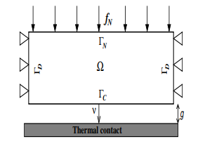
We describe in this section the numerical results we obtained for Problems 3 and 4 in dimension two. We consider the physical setting depicted in Figure 1. Let \(\Omega=(0,3)\times(0,1)\subset \mathbb{R}^2\) be a rectangle with boundary \(\Gamma\). On \(\Gamma_{D}= \{0\}\times [0,1]\cup \{3\}\times [0,1]\) the body is clamped. Vertical tractions act on \(\Gamma_N = [0, 3]\times\{1\}\). Affected by these forces, the body may contact with the foundation, on the contact surface \(\Gamma_{C}= [0,3]\times\{0\}\). We suppose that the temperature vanishes in \(\Gamma_D\cup\Gamma_N\).
The material response is governed by a thermoelastic linear constitutive law defined by the elasticity tensor \({\cal F}\) and the thermal expansion tensor \({\cal M}\) given by \[\begin{aligned} ({\cal F}{\tau})_{i j}&=\frac{E\nu}{1-\nu^2}(\tau_{11}+\tau_{22})\delta_{i j}+\frac{E}{1+\nu}\tau_{i j}, \quad 1\leq i,j\leq 2, \\ m_{i j} &= \alpha_{th} \frac{E}{1-2\nu}\delta_{i j}, \end{aligned}\] where \(E\) is the Young’s modulus, \(\nu\) is the Poisson’s ratio of the material, \(\delta_{i j}\) denotes the Kronecker symbol (\(\delta_{i j} = 1 \mbox{ if } i = j \mbox{ and } \delta_{i j} = 0 \mbox{ if } i \neq j\)) and \(\alpha_{th}\) is the thermal expansion coefficient.
The following data have been used in the numerical simulations: \[\begin{aligned} && E=10^4\, N/m^2,\; \nu=0.3,\; \alpha_{th} = 10^{-4}\, K^{-1},\; {k}_{i j} = 1.5 \delta_{i j} \, W/(m K),\\[1mm] &&\mathbf{f}_0 = \mathbf{0}\, N/m^2,\;q_0 = 0\, W/m^2,\; g = 10^{-1}\,m,\;\mathbf{f}_N(x,y) = (0,-10) \,N/m,\\[1mm] &&\epsilon = 10^{-8}\, N /m^2 ,\; \delta = 10^{-11}\, W /(m^2 K),\; \bar{k}_c= 1\, W/(N K),\; \theta_f = 15 \,K,\; \theta_{0} = 3 \,K. \end{aligned}\]
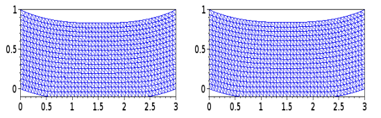
The deformed configuration of the body is represented in Figure 2 (left), which corresponds to the numerical solution of the penalty Problem 3. In order to compare the deformed mesh related to Problem 3 with that obtained for the numerical solution of Problem 4, we plotted in Figure 2 (right) the deformed configuration for the numerical solution of the Lagrangian Problem 4.
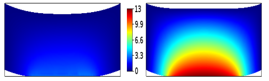
In Figure 3, the temperature field is plotted on the deformed configuration. Clearly, effects due to the compression, or the influence of foundation temperature, can be observed.
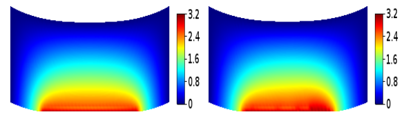
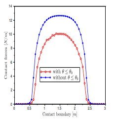
According to Figures 2-3, we observe that the numerical results obtained for the solution of the Lagrangian Problem 4 are very well approximated by the solution of the penalty Problem 3, provided that the penalty parameters takes very small values. Next, in order to highlight the influence of the temperature on the model, we plot the deformed meshes and the interface forces on \(\Gamma_C\) for two different cases, one with and the other without constraining condition \(\theta\leq \theta_{0} \mbox{ in } \Omega\). Note that in the case of the condition \(\theta\leq \theta_{0}\), the temperature’s contribution to the body’s deformation is small; therefore, the body is compressed by the actions of tractions. However, in the second case, when this condition is not considered in the model, the body’s shape changes significantly because of the temperature difference. Such a phenomenon is evident on the contact boundary: the contact forces’ magnitude decreases when the domain temperature decreases (see Figure 5).
In this paper, the thermoelastic contact problem is numerically studied. The novelties arise because the foundation is thermally conductive in which the heat exchange coefficient depends on the contact pressure. A discrete scheme was used to approach the problem, and a numerical algorithm was implemented. We report a comparison between numerical solutions of the double penalty problem and the Lagrangian one, shown in Figures 2-3. It shows that the solution of the contact problem with a rigid obstacle can be approached by the solution of a penalty contact problem, provided that the penalty parameters approach zero. As prospects, we plan to study further models of thermal contact with friction and wear.