
A double diffusive MHD flow of hybrid nanofluid has attracted many researchers recently in literature. The existence of heat-mass transmission (double diffusive) flow simultaneously in a flowing fluid greatly influences the fluid flow’s energy and mass flux. The energy flux due to the composition gradient is referred to as diffusion thermal or Dufour mechanism. Temperature gradient gives rise to mass fluxes which is referred to as thermal-diffusion or Soret effect. The effects of the Soret mechanism have been employed for the separation of isotopes. The significance of the Soret-Dufour mechanism on the dynamics of MHD convective nanofluids over a stretchable sheet has been investigated by Reddy and Chamkha [1]. Soret-Dufour mechanism on a Casson nano-fluid dynamics over a shrinking cylinder by varying Arrhenius activation energy and characteristics have been investigated by Shaheen et al. [2]. Srinivasacharya et al. [3] explained the Soret-Dufour mechanism towards a vertical wavy surface in a penetrable regime by varying properties. Pattnaik et al. [4] examined diffusion-thermal significance on hydromagnetic dynamics past an infinite vertical penetrable plate.
Vishala et al. [5] examined radiation and Marangoni convection on the dynamics of ternary nanofluid in a penetrable regime with mass transportation. Waqas et al. [6] elucidated the role of MHD radiatively dynamics of a hybrid nanofluid (HN) past a circular disk.. Ullah et al. [7] studied the thermal enhancement of ternary HN (Si2+Cu+MOS2/H2O) symmetric dynamics past a nonlinear stretchable regime. Soliman et al. [8] studied Rivlin-Ericksen nanofluid dynamics of radiative MHD third-grade fluid past a penetrable regime with a constant heat source. Sudarmozhi et al. [9] examined Maxwell fluid flow through a penetrable inclined slanting plate with convective heat and magneto radiative effects. The study of Hakeem et al. [10] explained 3D dissipative viscous systematics of nanofluids past a Riga plate. Irshad et al. [11] examined generalized Newtonian fluid dynamics past a stretchable sheet with MHD and penetrable regime. Vishalakshi et al. [12] explained the heat transmission process of MHD fluid system past a penetrating stretchable/shrinked sheet. Algehyne et al. [13] explained MHD fluid system over a bi-directional heated and convective regime with mass flux conditions. Shah et al. [14] explained the systematic flow of the swirl of Al+Mg+TiO2 ternary HN with PST and PHF heating conditions. Cattaneo-Christov models on heat-mass transmission of hybrid nanofluid have gained muchzattention in the literature. The Cattaneo-Christov double diffusive describes the thermal and solutal characteristics in mass-heat transfer. Khan et al. [15] studied nanofluid dynamics to enhance nanoparticle diffusion efficiently with C-CDDM. Chen et al. [16] examined the significance of Cattaneo-Christov double diffusion with the induced magnetic field of Maxwell ternary nanofluid dynamics. Hafeez et al. [17] studied the Cattaneo-Christov double diffusion theory on the dynamics of non-Newtonian Oldroyd-B nanofluid. The contribution of Haq et al. [18] explained the Cattaneo-Christov model of double diffusion for reactive chemically magnetized HN. In C-CDDM in magnetized second-grade nanofluid entropy optimization by varying mass diffusivity and thermal conductivity have been investigated by Chu et al. [19]. Shah et al. [20] examined electrical magnetite micropolar Casson ferrofluid over a stretchable/shrinking sheet by Cattaneo-Christov and thermal conductivity model. Upadhay et al. [21] studied heat and mass flux conditions on unsteady Eyring-Powell dusty nanofluid with a Cattaneo-Christov model past a stretching sheet. Zhang et al. [22] studied the upshot of melting heat transmission in a rotating Von Karman dynamics of gold-silver/engine oil hybrid nanofluid. Aldabesh et al. [23] elucidated variable thermal conductivity on Buongiorno nanofluid model within a parallel stretching sheet. Magnetized nanofluid thermal improvement for multiple shapes nanoparticles past a radiative rotating disk has been investigated by Adnan et al. [24]. Ijaz and Ayub [25] studied dual stratification and magnetic dipole simulation in ferromagnetic Maxwell fluid and radiative flow. Waqas et al. [26] explored the significance of surface-catalyzed reactions in SiO2-H2O nanofluid dynamics through penetrable media. Magnetized Casson nanofluid flow with second law analysis in a squeezing geometry through a penetrable medium has been investigated by Rashidi et al. [27]. Abo-Zaid et al. [28] studied MHD Powell-Eyring dusty nanofluid dynamics based on stretching surfaces with heat flux boundary conditions, Li et al. [29] investgated. Aspects of an induced magnetic field utilization for heat and mass transfer ferromagnetic hybrid nanofluid flow driven by pollutant concentration.
This research primarily aims to investigate the numerical simulation of the Cattaneo-Christov double diffusive ferromagnetic hybrid nanofluids flow with induced magnetic field, thermal radiation, and exothermic and endothermic chemical reactions. In addition, the significant impact of heat generation, thermal radiation, permeability, the inverse of magnetic Prandtl number, Soret-Dufour, and exothermic and endothermic chemical reactions on the temperature, velocity, and concentration of flow past a stretching surface is investigated. The model equations are represented by PDEs and were changed into ODEs using similarity transformation. The reduced ODEs are solved using the spectral relaxation method (SRM) to decouple and linearize the system of equations. This numerical technique gives highly accurate outcomes in the iteration procedure. The numerical procedure and graphical outcomes for temperature, velocity, and concentration are discussed and presented for pertinent flow parameters. To the best of our knowledge, no study in the literature has considered a mathematical model of this type. The present outcomes as compared with other studies are discovered to be in good agreement.
We explored the incompressible, laminar, two-dimensional, and steady flow of a hybrid nanofluid past a stretching/shrinking surface. The mass flux conditions and thermal convective conditions are considered in this research. An induced magnetic field is taken into consideration in this study. \(H^{\mathrm{*}}_{\mathrm{1}}\) and \(H^{\mathrm{*}}_{\mathrm{2}}\) is used to denote parallel and normal portions of the induced magnetic flux within the boundary layer. \(T_w\) and \(C_w\) are wall temperature and concentration while \(C_{\infty }\) and \(T_{\infty }\) are ambient concentration and temperature respectively. The stretching surface contained a velocity \(u^{\mathrm{*}}_e\mathrm{=}ax\) at the free stream and \(u_w\mathrm{(}x\mathrm{)=}cx\) at the wall \(\mathrm{(}a,c\mathrm{>0)}\). In addition, exothermic and endothermic chemical reaction equations were assumed significant in the concentration and temperature equations. All fluid properties are assumed constant while boundary layer approximation is considered to be valid. The governing equation becomes:
\[\label{GrindEQ__1_} \frac{\partial u_{\mathrm{1}}}{\partial x}+\frac{\partial u_{\mathrm{2}}}{\partial y}\mathrm{=0}, \tag{1}\]
\[\label{GrindEQ__2_} \frac{\partial H^{\mathrm{*}}_{\mathrm{1}}}{\partial x}+\frac{\partial H^{\mathrm{*}}_{\mathrm{2}}}{\partial y}\mathrm{=0} , \tag{2}\]
\[\label{GrindEQ__3_} u_{\mathrm{1}}\frac{\partial u_{\mathrm{1}}}{\partial x}+u_{\mathrm{2}}\frac{\partial u_{\mathrm{1}}}{\partial y}-\frac{{\mu }^{\mathrm{*}}_e}{\mathrm{4}{\rho }_{hnf}\pi }\left(H^{\mathrm{*}}_{\mathrm{1}}\frac{\partial H^{\mathrm{*}}_{\mathrm{1}}}{\partial x}+H^{\mathrm{*}}_{\mathrm{2}}\frac{\partial H^{\mathrm{*}}_{\mathrm{1}}}{\partial y}\right)\mathrm{=}u^{\mathrm{*}}_e\frac{du^{\mathrm{*}}_e}{dx}-\frac{{\mu }^{\mathrm{*}}_eH^{\mathrm{*}}_e}{\mathrm{4}{\rho }_{hnf}\pi }\frac{dH^{\mathrm{*}}_e}{dx}+{\nu }_{hnf}\frac{{\partial }^{\mathrm{2}}u_{\mathrm{1}}}{\partial y^{\mathrm{2}}}-\frac{{\mu }_{hnf}}{K}u_{\mathrm{1}} , \tag{3}\]
\[\label{GrindEQ__4_} u_{\mathrm{1}}\frac{\partial H^{\mathrm{*}}_{\mathrm{1}}}{\partial x}+u_{\mathrm{2}}\frac{\partial H^{\mathrm{*}}_{\mathrm{1}}}{\partial y}\mathrm{=}H^{\mathrm{*}}_{\mathrm{1}}\frac{\partial u_{\mathrm{1}}}{\partial x}+H^{\mathrm{*}}_{\mathrm{2}}\frac{\partial u_{\mathrm{1}}}{\partial y}+{\eta }_0\frac{{\partial }^{\mathrm{2}}H^{\mathrm{*}}_{\mathrm{1}}}{\partial y^{\mathrm{2}}} , \tag{4}\]
\[\begin{aligned} \label{GrindEQ__5_} u_1 \frac{\partial T}{\partial x} +& u_2 \frac{\partial T}{\partial y} = \alpha_{hnf} \frac{\partial^2 T}{\partial y^2} + \frac{Q}{\rho c_p} (T – T_{\infty}) – \frac{1}{(\rho c_p)_{hnf}} \frac{\partial q_r}{\partial y} + \frac{D K_T}{c_s c_p} \frac{\partial^2 C}{\partial y^2} + \beta K_r^2 \left(\frac{T}{T_{\infty}}\right)^n \exp\left(\frac{-E_a}{K T}\right) (C – C_{\infty}) \nonumber \\ &\quad – h_1 \Bigg[ u_1 \frac{\partial u_1}{\partial x} \frac{\partial T}{\partial x} + u_2 \frac{\partial u_2}{\partial y} \frac{\partial T}{\partial x} + u_1 \frac{\partial u_2}{\partial x} \frac{\partial T}{\partial x} + (u_2)^2 \frac{\partial^2 T}{\partial y^2} + u_2 \frac{\partial u_1}{\partial y} \frac{\partial T}{\partial x} + 2 u_1 u_2 \frac{\partial^2 T}{\partial y \partial x} + (u_2)^2 \frac{\partial^2 T}{\partial y^2} \Bigg], \end{aligned} \tag{5}\]
\[\begin{aligned} \label{GrindEQ__6_} u_1 \frac{\partial C}{\partial x} +& u_2 \frac{\partial C}{\partial y} = D_m \frac{\partial^2 C}{\partial y^2} + \frac{D K_T}{T_m} \frac{\partial^2 T}{\partial y^2} – K_r^2 \left(\frac{T}{T_{\infty}}\right)^n \exp\left(\frac{-E_a}{K T}\right) (C – C_{\infty}) + S(C) \nonumber \\ &\quad – h_1 \Bigg[ u_1 \frac{\partial u_1}{\partial x} \frac{\partial C}{\partial x} + u_2 \frac{\partial u_2}{\partial y} \frac{\partial C}{\partial x} + u_1 \frac{\partial u_2}{\partial x} \frac{\partial C}{\partial x} + (u_2)^2 \frac{\partial^2 C}{\partial y^2} + u_2 \frac{\partial u_1}{\partial y} \frac{\partial C}{\partial x} + 2 u_1 u_2 \frac{\partial^2 C}{\partial y \partial x} + (u_2)^2 \frac{\partial^2 C}{\partial y^2} \Bigg], \end{aligned} \tag{6}\] Subject to: \[\label{GrindEQ__7_} u_{\mathrm{1}}\mathrm{=}u_w\mathrm{(}x\mathrm{)=}cx,\ \ v\mathrm{=0,}\ \ \frac{\partial H^{\mathrm{*}}_{\mathrm{1}}}{\partial y}\mathrm{=}H^{\mathrm{*}}_{\mathrm{2}}\mathrm{=0,}\ \ T\mathrm{=}T_w,\ \ \ \ C\mathrm{=}C_w\mathrm{::}\ \ \ \ \ \ y\mathrm{=0} , \tag{7}\]
\[\label{GrindEQ__8_} u_{\mathrm{1}}\mathrm{=}u^{\mathrm{*}}_e\mathrm{=}ax,\ \ H^{\mathrm{*}}_{\mathrm{1}}\mathrm{=}H^{\mathrm{*}}_e,\ \ T\mathrm{=}T_{\infty },\ \ \ \ C\mathrm{=}C_{\infty }\mathrm{:}\ \ \ \ \ \ y\mathrm{\longrightarrow }\infty , \tag{8}\] where \(u_1\) and \(u_2\) are velocity components, D is mass diffusivity, \(\alpha\) means thermal diffusivity, x and y are coordinates, \(H^*_1\) and \(H^*_2\) are induced magnetism vectors, k means Boltzmann constant, \(E_a\) is activation energy, S(C) means external pollutant source function, n means fitted rate constant, \(K^2_r\) is the rate of limiting factor for the chemical process, \(\beta\) is the endothermic and exothermic factor, T and C are temperature and concentration, \({\eta }_0\) means magnetic diffusivity, \(\nu\) means kinematic viscosity, \({\mu }^*_e\) is the magnetic permeability, \(H^*_e\) means free stream magnetic fields, \(T_{\infty }\) and \(C_{\infty }\) are free stream temperature and concentration respectively, \({\lambda }_2\) and \(Q_1\) are external pollutant concentration as well as pollutant source external variation parameter. Physical configuration of the model is given in Figure 1.

The similarity variables are defined as: \[\begin{aligned} u_1=&xcf\left(\eta \right),\ u_2=-f\left(\eta \right)\sqrt{{\nu }_fc},\ \eta =y\sqrt{\frac{c}{{\nu }_f}},\ H^*_1=H_0\left(\frac{x}{l}\right)g'\left(\eta \right),\\ H^*_2=&-g\left(\eta \right)H_0\sqrt{\frac{{\nu }_f}{l^2c}},\ \theta =\frac{T-T_{\infty }}{T_w-T_{\infty }}, \varphi =\frac{C-C_{\infty }}{C_w-C_{\infty }}. \end{aligned}\] The transformed ODEs are given as follows after the implementation of the similarity variables:
\[\label{GrindEQ__9_} \frac{\mathrm{1}}{{\omega }_{\mathrm{1}}}f'''+{\omega }_{\mathrm{2}}\left(ff''-\mathrm{(}f'{\mathrm{)}}^{\mathrm{2}}+\mathrm{(}A^{\mathrm{*}}{\mathrm{)}}^{\mathrm{2}}\right)+M\left(\mathrm{(}g'{\mathrm{)}}^{\mathrm{2}}-gg''-\mathrm{1}\right)-\frac{\mathrm{1}}{Po}f'\mathrm{=0} , \tag{9}\]
\[\label{GrindEQ__10_} {\lambda }^{\mathrm{*}}g'''+g''f-gf''\mathrm{=0} , \tag{10}\]
\[\label{GrindEQ__11_} \frac{K_{hnf}}{K_f}\left(\frac{\mathrm{1}+R}{Pr}\right){\theta }''+{\omega }_{\mathrm{3}}\left(f\theta '+Qo\theta +Do\varphi ''+{\lambda }_{\mathrm{1}}{\sigma }^{\mathrm{*}}\mathrm{(}\delta \theta +\mathrm{1}{\mathrm{)}}^nexp\left(-\frac{E^{\mathrm{*}}}{\delta \theta +\mathrm{1}}\right)\varphi \right)-{\beta }_0\mathrm{(}ff'\theta '+f^{\mathrm{2}}\theta ''\mathrm{)=0} , \tag{11}\]
\[\label{GrindEQ__12_} \varphi ''+Sc\left(\varphi 'f-{\sigma }^{\mathrm{*}}\mathrm{(}\delta \theta +\mathrm{1}{\mathrm{)}}^nexp\left(-\frac{E^{\mathrm{*}}}{\delta \theta +\mathrm{1}}\right)\varphi +{\beta }^{\mathrm{*}}_{\mathrm{1}}exp\mathrm{(}\varphi B\mathrm{)}\right)-{\beta }_{\mathrm{1}}\mathrm{(}ff'\varphi '+f^{\mathrm{2}}\varphi ''\mathrm{)=0} . \tag{12}\] Subject to:
\[\label{GrindEQ__13_} f\mathrm{=0,}\ \ \ \ f'\mathrm{=1,}\ \ \ \ g\mathrm{=0,}\ \ \ \ g''\mathrm{=0,}\ \ \ \ \varphi \mathrm{=1,}\ \ \ \ \theta \mathrm{=1,}\ \ \ \ \eta \mathrm{=0} , \tag{13}\]
\[\label{GrindEQ__14_} f'\mathrm{=}A^{\mathrm{*}},\ \ \ \ g'\mathrm{=1,}\ \ \ \ \varphi \mathrm{=0,}\ \ \ \ \theta \mathrm{=0,}\ \ \ \ \ \ \eta \mathrm{\longrightarrow }0 . \tag{14}\]
The parameters involved in this analysis are defined as: \(M\mathrm{=}\frac{{\mu }^{\mathrm{*}}_eH^{\mathrm{2}}_0}{\mathrm{4}\pi c^{\mathrm{2}}l^{\mathrm{2}}{\rho }_f}\) is magnetism parameter, \(Po\mathrm{=}\frac{{\mu }_{hnf}}{k\rho }\) is permeability parameter, \({\lambda }^{\mathrm{*}}\mathrm{=}\frac{{\eta }_0}{{\nu }_f}\) is inverse of magnetic Prandtl number, \(R\mathrm{=}\frac{\mathrm{4}{\sigma }_0T^{\mathrm{3}}_{\infty }}{\mathrm{3}kek^{\mathrm{*}}}\) is thermal radiation parameter, \(Pr\mathrm{=}\frac{{\nu }_f}{{\alpha }_f}\) is Prandtl number, \(Qo\mathrm{=}\frac{Q}{\rho c_pa}\) is heat generation term, \(A^{\mathrm{*}}\mathrm{=}\frac{a}{c}\) is velocity ratio parameter, \(Do\mathrm{=}\frac{Dk_T\mathrm{(}C_w-C_{\infty }\mathrm{)}}{c_sc_p\nu \mathrm{(}T_w-T_{\infty }\mathrm{)}}\) is Dufour term, \({\lambda }_{\mathrm{1}}\mathrm{=}\beta \frac{\mathrm{(}C_w-C_{\infty }\mathrm{)}}{\mathrm{(}T_w-T_{\infty }\mathrm{)}}\) is an endothermic or exothermic parameter, \(\delta \mathrm{=}\frac{T_w-T_{\infty }}{T_{\infty }}\) is temperature difference parameter, \(E^{\mathrm{*}}\mathrm{=}\frac{Ea}{kT_{\infty }}\) is activation energy parameter, \(Sc\mathrm{=}\frac{{\nu }_f}{D_f}\) is Schmidt number, \(So\mathrm{=}\frac{Dk_T\mathrm{(}T_w-T_{\infty }\mathrm{)}}{T_m\nu \mathrm{(}C_w-C_{\infty }\mathrm{)}}\) is Soret term, \({\sigma }^{\mathrm{*}}\mathrm{=}\frac{k^{\mathrm{2}}_r}{c}\) is a chemical reaction parameter, \({\beta }^{\mathrm{*}}_{\mathrm{1}}\mathrm{=}\frac{{\lambda }_{\mathrm{2}}}{c\mathrm{(}C_w-C_{\infty }\mathrm{)}}\) is a pollutant external source, \(B\mathrm{=}Q_{\mathrm{1}}\mathrm{(}C_w-C_{\infty }\mathrm{)}\) is external pollutant source variation.
\[\begin{aligned} {\omega }_1=&{\left(1-{\varphi }_1\right)}^{2.5}{\left(1-{\varphi }_2\right)}^{2.5},\\ {\omega }_2=&\left\{\left(1-{\varphi }_2\right)[\left(1-{\varphi }_1\right)+\frac{{\varphi }_1{\rho }_{s1}}{{\rho }_f}]\right\}+\frac{{\varphi }_2{\rho }_{s2}}{{\rho }_f} , \\ {\omega }_3=&\left\{\left(1-{\varphi }_2\right)[\left(1-{\varphi }_1\right)+\frac{{\varphi }_1{\left(\rho c_p\right)}_{s1}}{{\left(\rho c_p\right)}_f}]\right\}+\frac{{\varphi }_2{\left(\rho c_p\right)}_{s2}}{{\left(\rho c_p\right)}_f}. \end{aligned}\]
| Property | Symbol | Mathematical expression |
| Density | \(\rho \) | \(\rho _hnf=\left\{\left(1-\varphi _2\right)[\rho _f\left(1-\varphi _1\right)+\rho _s1\varphi _1]\right\}+\varphi _2\rho _s2\) |
| Dynamic viscosity | \(\mu \) | \(\mu _hnf=\frac{{\mu }_f{(1-{\varphi }_2)}^{-2.5}}{{(1-{\varphi }_1)}^{2.5}}\) |
| Thermal conductivity | \(k\) | \(\frac{k_{hnf}}{k_{nf}}=\frac{k_{s_2}+2k_{nf}-2{\varphi }_1(k_{nf}-k_{s_2})}{k_{s_2}+2k_{nf}+{\varphi }_2(k_{nf}-k_{s_2})} \quad \frac{k_{nf}}{k_f}=\frac{k_{s_1}+2k_f-2{\varphi }_1(k_f-k_{s_1})}{k_{s_1}+2k_f+{\varphi }_1(k_f-k_{s_1})}\) |
| Heat capacity | \(\rho c_p\) | \({\left(\rho c_p\right)}_{hnf}=\left\{\left(1-{\varphi }_2\right)[{\left(\rho c_p\right)}_f\left(1-{\varphi }_1\right)+{{\left(\rho c_p\right)}_f}_{s1}{\varphi }_1]\right\}+{\varphi }_2{{\left(\rho c_p\right)}_f}_{s2}\) |
The dimensionless transformed equations have been tackled with SRM. The choice of this technique is due to its ability to decouple as well as linearizing the set of Eqs. (9)-(12) by utilizing, the Chebyshev spectral technique. The SRM is very easy to compute with a very high accuracy. In the SRM numerical simulations, the most recent iteration are done at \(r+\mathrm{1}\) while previous iteration is conducted at \(r\). The SRM as utilized on the transformed equations are described as follows:
\[\label{GrindEQ__15_} \frac{\mathrm{1}}{{\omega }_{\mathrm{1}}}{f'''}_{r+\mathrm{1}}+{\omega }_{\mathrm{2}}f_r{f''}_{r+\mathrm{1}}-{\omega }_{\mathrm{2}}\mathrm{(}{f'}_{r+\mathrm{1}}{\mathrm{)}}^{\mathrm{2}}+{\omega }_{\mathrm{2}}\mathrm{(}A^{\mathrm{*}}{\mathrm{)}}^{\mathrm{2}}+{\beta }^{\mathrm{*}}\mathrm{(}{g'}_r{\mathrm{)}}^{\mathrm{2}}-{\beta }^{\mathrm{*}}g_r{g''}_r-{\beta }^{\mathrm{*}}-\frac{\mathrm{1}}{Po}{f'}_{r+\mathrm{1}}\mathrm{=0} , \tag{15}\]
\[\begin{aligned} \label{GrindEQ__16_} &\frac{K_{hnf}}{K_f} \left(\frac{1+R}{Pr} \right) \theta''_{r+1} + \omega_3 f_{r+1} \theta'_{r+1} + \omega_3 Q_0 \theta_{r+1} + \omega_3 D_0 \varphi''_r \nonumber \\ & + \omega_3 \lambda_1 \sigma^* (\delta \theta_r + 1)^n \exp\left(-\frac{E^*}{\delta \theta_{r+1}}\right) \varphi_{r+1} – \omega_3 \beta_0 f_r f'_r \theta'_{r+1} – \omega_3 f_r^2 \theta''_{r+1} = 0, \end{aligned} \tag{16}\]
\[\label{GrindEQ__17_} {\lambda }^{\mathrm{*}}{g'''}_{r+\mathrm{1}}+f_{r+\mathrm{1}}{g''}_{r+\mathrm{1}}-g_{r+\mathrm{1}}{f''}_r\mathrm{=0} , \tag{17}\]
\[\begin{aligned} \label{GrindEQ__18_} &\varphi''_{r+1} + Sc f_{r+1} \varphi'_{r+1} – Sc \sigma^* (\delta \theta_{r+1} + 1)^n \exp\left(-\frac{E^*}{\delta \theta_{r+1+1}}\right) \varphi_{r+1} \nonumber \\ & + Sc \beta_1^* \exp(\Delta, B) – Sc \beta_1 f_r f'_r \varphi'_{r+1} – Sc \beta_1 f_r^2 \varphi''_{r+1} = 0. \end{aligned} \tag{18}\] The coefficient parameters are defined as follows: \[\begin{aligned} a_{0,r}\mathrm{=}&{\omega }_{\mathrm{2}}f_r,\\ a_{\mathrm{1,}r}\mathrm{=}&-{\omega }_{\mathrm{2}}\mathrm{(}{f'}_{r+\mathrm{1}}{\mathrm{)}}^{\mathrm{2}}, \\ a_{\mathrm{2,}r}\mathrm{=}&-{\beta }^{\mathrm{*}}{\omega }_{\mathrm{2}}\mathrm{(}A^{\mathrm{*}}{\mathrm{)}}^{\mathrm{2}},\\ a_{\mathrm{3,}r}\mathrm{=}&-{\beta }^{\mathrm{*}}g_r{g''}_r,\\ a_{\mathrm{4,}r}\mathrm{=}&{\beta }^{\mathrm{*}}\mathrm{(}{g'}_r{\mathrm{)}}^{\mathrm{2}},\\ b_{0,r}\mathrm{=}&\frac{K_{hnf}}{K_f}\left(\frac{\mathrm{1}+R}{Pr}\right),\\ b_{\mathrm{1,}r}\mathrm{=}&{\omega }_{\mathrm{3}}f_{r+\mathrm{1}},\\ b_{\mathrm{2,}r}\mathrm{=}&{\omega }_{\mathrm{3}}Qo,\\ b_{\mathrm{3,}r}\mathrm{=}&{\omega }_{\mathrm{3}}Do{\varphi ''}_r,\\ b_{\mathrm{4,}r}\mathrm{=}&{\omega }_{\mathrm{3}}{\lambda }_{\mathrm{1}}{\sigma }^{\mathrm{*}}\mathrm{(}\delta {\theta }_{r+\mathrm{1}}{\mathrm{)}}^nexp\left(-\frac{E^{\mathrm{*}}}{\delta {\theta }_{r+\mathrm{1}}}+\mathrm{1}\right),\\ b_{\mathrm{5,}r}\mathrm{=}&-{\omega }_{\mathrm{3}}{\beta }_of_r{f'}_r,\\ b_{\mathrm{6,}r}\mathrm{=}&-{\omega }_{\mathrm{3}}f^{\mathrm{2}}_r\\ c_{0,r}\mathrm{=}&f_{r+\mathrm{1}},\\ c_{1,r}\mathrm{=}&{f''}_r,\\ d_{0,r}\mathrm{=}&Scf_{r+\mathrm{1}},\\ d_{\mathrm{1,}r}\mathrm{=}&-Sc{\sigma }^{\mathrm{*}}\mathrm{(}\delta {\theta }_{r+\mathrm{1}}+\mathrm{1}{\mathrm{)}}^nexp\left(-\frac{E^{\mathrm{*}}}{\delta {\theta }_{r+\mathrm{1}}+\mathrm{1}}\right),\\ \\d_{\mathrm{4,}r}\mathrm{=}&Sc{\beta }^{\mathrm{*}}_{\mathrm{1}}exp\mathrm{(}{\varphi }_rB\mathrm{),}\\ d_{\mathrm{2,}r}\mathrm{=}&-Sc{\beta }_{\mathrm{1}}f_rf_{r+\mathrm{1}},\\ d_{\mathrm{3,}r}\mathrm{=}&-Sc{\beta }_{\mathrm{1}}f^{\mathrm{2}}_r. \end{aligned}\] Substituting the coefficient parameters above to obtain:
\[\label{GrindEQ__19_} \frac{\mathrm{1}}{{\omega }_{\mathrm{1}}}{f'''}_{r+\mathrm{1}}+a_{0,r}{f''}_{r+\mathrm{1}}+a_{\mathrm{1,}r}+a_{\mathrm{2,}r}+a_{\mathrm{4,}r}+a_{\mathrm{3,}r}-\frac{\mathrm{1}}{Po}{f'}_{r+\mathrm{1}}\mathrm{=0} , \tag{19}\]
\[\label{GrindEQ__20_} b_{0,r}{\theta ''}_{r+\mathrm{1}}+b_{\mathrm{1,}r}{\theta '}_{r+\mathrm{1}}+b_{\mathrm{2,}r}{\theta }_{r+\mathrm{1}}+b_{\mathrm{3,}r}+b_{\mathrm{4,}r}+b_{\mathrm{5,}r}{\theta '}_{r+\mathrm{1}}+b_{\mathrm{6,}r}{\theta ''}_{r+\mathrm{1}}\mathrm{=0} , \tag{20}\]
\[\label{GrindEQ__21_} {\lambda }^{\mathrm{*}}{g'''}_{r+\mathrm{1}}+c_{0,r}{g''}_{r+\mathrm{1}}-c_{\mathrm{1,}r}g_{r+\mathrm{1}}\mathrm{=0} , \tag{21}\]
\[\label{GrindEQ__22_} {\varphi ''}_{r+\mathrm{1}}+d_{0,r}{\varphi '}_{r+\mathrm{1}}+d_{\mathrm{1,}r}{\varphi }_{r+\mathrm{1}}+d_{\mathrm{4,}r}+d_{\mathrm{2,}r}{\varphi '}_{r+\mathrm{1}}+d_{\mathrm{3,}r}{\varphi ''}_{r+\mathrm{1}}\mathrm{=0} , \tag{22}\]
\[\label{GrindEQ__23_} \left[\frac{\mathrm{1}}{{\omega }_{\mathrm{1}}}D^{\mathrm{3}}+a_{\mathrm{0,1}}D^{\mathrm{2}}-\frac{\mathrm{1}}{Po}D\right]f_{r+\mathrm{1}}+a_{\mathrm{1,}r}+a_{\mathrm{2,}r}+a_{\mathrm{3,}r}+a_{\mathrm{4,}r}\mathrm{=0} , \tag{23}\]
\[\label{GrindEQ__24_} \left[b_{0,r}D^{\mathrm{2}}+b_{\mathrm{1,}r}D+b_{\mathrm{2,}r}+b_{\mathrm{5,}r}D+b_{\mathrm{6,}r}D^{\mathrm{2}}\right]{\theta }_{r+\mathrm{1}}+b_{\mathrm{3,}r}+b_{\mathrm{4,}r}\mathrm{=0} , \tag{24}\]
\[\label{GrindEQ__25_} \left[{\lambda }^{\mathrm{*}}D^{\mathrm{3}}+c_{0,r}D^{\mathrm{2}}-c_{\mathrm{1,}r}\right]g_{r+\mathrm{1}}\mathrm{=0} , \tag{25}\]
\[\label{GrindEQ__26_} \left[D^{\mathrm{2}}+d_{0,r}D+d_{\mathrm{1,}r}+d_{\mathrm{2,}r}D+d_{\mathrm{3,}r}D^{\mathrm{2}}\right]{\varphi }_{r+\mathrm{1}}+d_{\mathrm{4,}r}\mathrm{=0} . \tag{26}\]
To implement the SRM, the following initial approximation is defined in accordance to the boundary constraints as: \[\label{GrindEQ__27_} f_0\mathrm{(}\eta \mathrm{)=1}-e^{-\eta },{f'}_0\mathrm{(}\eta \mathrm{)=}{\theta }_0\mathrm{(}\eta \mathrm{)=}{\varphi }_0\mathrm{(}\eta \mathrm{)=}e^{-\eta },g_0\mathrm{(}\eta \mathrm{)=1}-e^{-\eta } . \tag{27}\]
The implicit difference technique is further utilized in the dimensionless distance \(\mathrm{(}\eta \mathrm{)}\) direction. The scheme is defined as follows:
\[\label{GrindEQ__28_} \varphi \mathrm{(}\eta \mathrm{)=}\frac{{\varphi }^{n+\mathrm{1}}_j+{\varphi }^n_j}{\mathrm{2}},\ \ f\mathrm{(}\eta \mathrm{)=}\frac{f^{n+\mathrm{1}}_j+f^n_j}{\mathrm{2}},\ \ \theta \mathrm{(}\eta \mathrm{)=}\frac{{\theta }^{n+\mathrm{1}}_j+{\theta }^n_j}{\mathrm{2}},\ \ g\mathrm{(}\eta \mathrm{)=}\frac{g^{n+\mathrm{1}}_j+g^n_j}{\mathrm{2}} . \tag{28}\]
Applying the finite difference scheme to obtain
\[\label{GrindEQ__29_} \left(\frac{{\omega }_{\mathrm{1}}D^{\mathrm{3}}+a_{\mathrm{0,1}}D^{\mathrm{2}}-\frac{\mathrm{1}}{Po}D}{\mathrm{2}}\right)f^{n+\mathrm{1}}_j\mathrm{=}-\left(\frac{{\omega }_{\mathrm{1}}D^{\mathrm{3}}+a_{\mathrm{0,1}}D^{\mathrm{2}}-\frac{\mathrm{1}}{Po}D}{\mathrm{2}}\right)f^n_j-a^{n+\mathrm{1}}_{\mathrm{1,}r}-a^{n+\mathrm{1}}_{\mathrm{2,}r}-a^{n+\mathrm{1}}_{\mathrm{3,}r}-a^{n+\mathrm{1}}_{\mathrm{4,}r} , \tag{29}\]
\[\label{GrindEQ__30_} \left(\frac{b_{0,r}D^{\mathrm{2}}+b_{\mathrm{1,}r}D+b_{\mathrm{2,}r}+b_{\mathrm{5,}r}D+b_{\mathrm{6,}r}D^{\mathrm{2}}}{\mathrm{2}}\right){\theta }^{n+\mathrm{1}}_j\mathrm{=}-\left(\frac{b_{0,r}D^{\mathrm{2}}+b_{\mathrm{1,}r}D+b_{\mathrm{2,}r}+b_{\mathrm{5,}r}D+b_{\mathrm{6,}r}D^{\mathrm{2}}}{\mathrm{2}}\right){\theta }^n_j-b^{n+\mathrm{1}}_{\mathrm{3,}r}-b^{n+\mathrm{1}}_{\mathrm{4,}r}, \tag{30}\]
\[\label{GrindEQ__31_} \left(\frac{{\lambda }^{\mathrm{*}}D^{\mathrm{3}}+c_{0,r}D^{\mathrm{2}}-c_{\mathrm{1,}r}}{\mathrm{2}}\right)g^{n+\mathrm{1}}_j\mathrm{=}-\left(\frac{{\lambda }^{\mathrm{*}}D^{\mathrm{3}}+c_{0,r}D^{\mathrm{2}}-c_{\mathrm{1,}r}}{\mathrm{2}}\right)g^n_j , \tag{31}\]
\[\label{GrindEQ__32_} \left(\frac{D^{\mathrm{2}}+d_{0,r}D+d_{\mathrm{1,}r}+d_{\mathrm{2,}r}D+d_{\mathrm{3,}r}D^{\mathrm{2}}}{\mathrm{2}}\right){\varphi }^{n+\mathrm{1}}_j\mathrm{=}-\left(\frac{D^{\mathrm{2}}+d_{0,r}D+d_{\mathrm{1,}r}+d_{\mathrm{2,}r}D+d_{\mathrm{3,}r}D^{\mathrm{2}}}{\mathrm{2}}\right){\varphi }^n_j-d^{n+\mathrm{1}}_{\mathrm{4,}r} . \tag{32}\]
From the above Eqs. (29)-(32), the following scheme is obtained:
\[\label{GrindEQ__33_} {\alpha }_{\mathrm{1}}f^{n+\mathrm{1}}_j\mathrm{=}{\beta }_{\mathrm{1}}f^n_j+K_{\mathrm{1}} , \tag{33}\] \[\label{GrindEQ__34_} {\alpha }_{\mathrm{2}}{\theta }^{n+\mathrm{1}}_j\mathrm{=}{\beta }_{\mathrm{2}}{\theta }^n_j+K_{\mathrm{2}} , \tag{34}\] \[\label{GrindEQ__35_} {\alpha }_{\mathrm{3}}g^{n+\mathrm{1}}_j\mathrm{=}{\beta }_{\mathrm{3}}g^n_j+K_{\mathrm{3}} , \tag{35}\] \[\label{GrindEQ__36_} {\alpha }_{\mathrm{4}}{\varphi }^{n+\mathrm{1}}_j\mathrm{=}{\beta }_{\mathrm{4}}{\varphi }^n_j+K_{\mathrm{4}} . \tag{36}\]
The solution to Eqs. (25)-(28) is obtained from the initial approximation in Eq. (19) iteratively. Also, Eqs. (15)-(18) are discretized with the means of Chebyshev collocation technique. A scaling parameter \(L\) is utilized to tackled the boundary constraints at infinity.
The analysis examined in this paper explained the impact of Cattaneo-Christov double diffusive flow of ferromagnetic HN with thermal radiation, heat generation and induced magnetic field. The numerical value of pertinent flow parameters such as heat relaxation flux \(\left({\beta }_1\right)\), chemical reaction parameter \(\left({\sigma }^*\right)\), Schmidt number (Sc), inverse of magnetism Prandtl term \(\left({\lambda }^*\right)\), magnetism term (M), permeability term (Po), and activation energy \(\left(E^*\right)\). The numerical value of this parameters are: \({\beta }_1=3.0,\ {\sigma }^*=0.6,\ Sc=0.61,\ {\beta }_0=3.0,\ {\lambda }^*=0.9,\ \ M=1.0,\ Po=0.8\) and \(E^*=0.5\).


Figure 2 shows the role of mass relaxation flux parameter \(\left({\beta }_0\right)\) on the velocity and concentration profile. A drastic enhancement in the fluid concentration is noticeable as \({\beta }_0\) increases. From the boundary layer where the dimensionless distance \(\eta =2.5\), there is no significant effect of \({\beta }_0\) on the flow. In Figure 2, higher value of \({\beta }_0\) was found to degenerates the velocity contour. This decrease in fluid velocity was due to the diffusion of fluxes within the layer. Figure 3 illustrate the effect of heat relaxation flux. The heat fluxes in the diffusive flow brings an increase in fluid velocity \(\left(g'\right)\) and temperature respectively. This significant effect are noticed on the fluid temperature very close to the plate. Figure 4 represents the impact of activation energy on the activation energy parameter \(\left(E^*\right)\) on the temperature together with velocity contour. The temperature contour in figure 4 shows increase in \(E^*\) shows increase in \(E^*\) drastically close to the vertical wall while it decreases small at the boundary layer. Increase in the magnitude of \(E^*\) decreases the velocity profile.
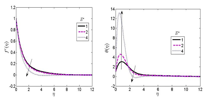

Figure 5 represents the role of the inverse of magnetic Prandtl \(\left({\lambda }^*\right)\) on the concentration and velocity contour respectively. A higher \({\lambda }^*\) was found to decline the concentration contour close to the wall and raise the contour at the boundary layer. Physically, the magnetism is capable of increasing the profile due to its origination of Lorentz force. This force depreciates the movement of an electrically fluid conducting. The higher value of \({\lambda }^*\) degenerates the velocity contour.
Figure 6 represents the impact of magnetism (M) on the induced velocity \(\left(g'\right)\) and temperature contour. Magnetism induced currents to the boundary layer. This current produces magnetic forces which decreases the movement of a conducting fluid. This force can decrease the thickness of the hydrodynamic layer. The Lorentz force depletes the fluid velocity because of the imposed force on the boundary layer. In Figure 6, a higher M declines the fluid temperature because of the increased force of Lorentz. Figure 7 shows the role of the permeability term (Po) on the fluid temperature and velocity. The scenario of a permeable surface permits the fluid particles to move within the layer. This movement of fluid within the layer gives rise to a spontaneous collision of fluid particles. This resulted to an upsurge in fluid velocity when the magnitude of Po increases. As a result of the increasing value of Po, the fluid temperature degenerates within the boundary layer.
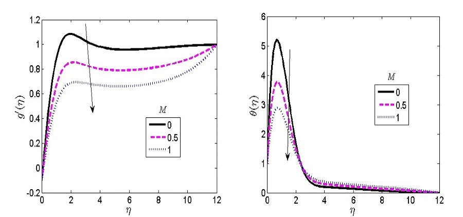

Figure 8 explains the role of Schmidt (Sc) on the velocity alongside concentration contour. A large value of Sc was found to decrease the fluid concentration. On the other hand, raising Sc was found to enhance the fluid velocities. The present analysis shows that the momentum spread is higher than the concentration spread. Physically, Sc=0 means the absence of mass flux and rate of mass transfer has been ignored. Hence, the model equation becomes mass transfer. Figure 9 depicts the role of the chemical reaction term \(\left({\sigma }^*\right)\) on the velocity alongside concentration contour respectively. The \({\sigma }^*\) is employed in transforming a chemical substance into another chemical substance. The chemical reaction activities in this model involve the nanoparticles and the controlled fluid parameters. A higher value of \({\sigma }^*\) was found to drastically increase the fluid velocity close to the wall. However, a higher value of \({\sigma }^*\) was found to decrease the fluid concentration profile. This implies a destructive chemical reaction in the fluid flow process.


The current analysis elucidated the significance of the Cattaneo-Christov double diffusive flow of ferromagnetic hybrid nanofluids past a stretching regime. The model was considered with flow parameters such as heat generation, thermal radiation, heterogeneous-homogeneous chemical reaction, and Soret-Dufour mechanisms. The model was obtained in the form of PDEs and was changed into ODEs through the help of transformational variables. The set of transformed ODEs was solved by using the SRM approach. This approach is employed to solve the equations iteratively. The key findings are stated as follows:
An upsurge in the chemical reaction was observed to increase the fluid velocity.
The magnetism field emanates Lorentz force which depletes the fluid velocity alongside the hydrodynamic boundary layer thickness.
Raising Sc was found to depreciate the fluid concentration but produces a higher profile on velocity profiles.
Raising the permeability term gives rise to a spontaneous collision of fluid particles which enhances the fluid velocity and decreases the fluid temperature.
The upsurge of mass relaxation fluid term was detected to increase the fluid concentration profile; and
The fluid velocity and temperature were found to increase because of a higher value of the heat relaxation flux parameter.