
An illegal act or omission that is penalized by the state under current laws is called a crime. It refers to conduct that violates laws established to protect individuals and society, for which the government has the authority to impose sanctions such as fines, imprisonment, or other penalties. Section 40 of the Indian Penal Code (IPC), 1860 defines an offense as any act or omission that is punishable by law. Furthermore, Black’s Law Dictionary describes crime as “an act that the law makes punishable; the breach of a legal duty treated as a criminal offense.” Crime remains a major social issue in India and across the world. Empirical data provide valuable insights into the trends, patterns, and challenges associated with crime management.
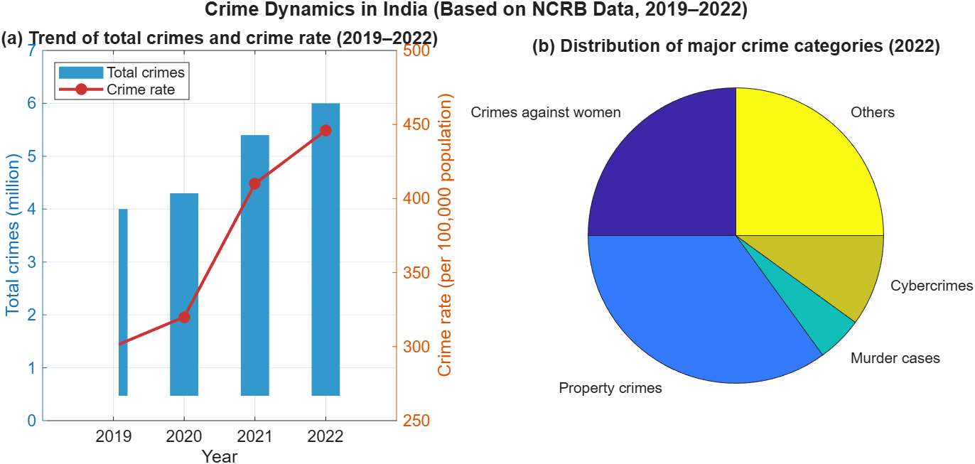
Understanding crime dynamics in India is crucial for effective policymaking. According to the National Crime Records Bureau (NCRB), in 2019 (see Figure 1), India reported approximately 4 million criminal cases, with a crime rate of around 300 per 100,000 population. Urban centers, in particular, exhibited a higher concentration of habitual offenders. Economic challenges also play a significant role, as World Bank estimates indicate that nearly 22% of the population lives below the poverty line, which may contribute to criminal activities. Recent NCRB data from 2022 show that nearly 6 million (60 lakh) cognizable crimes were registered under the Indian Penal Code (IPC) and Special and Local Laws (SLL), with an overall crime rate of about 445.9 per lakh population. Major reported crimes included around 4.5 lakh cases against women, numerous property-related offenses, and nearly 30,000 murder cases annually. Additionally, cybercrime incidents rose by more than 24% compared to the previous year. These statistics highlight the growing complexity of criminal behavior in India and emphasize the urgent need for robust mathematical and data-driven models to design effective crime prevention and control strategies.
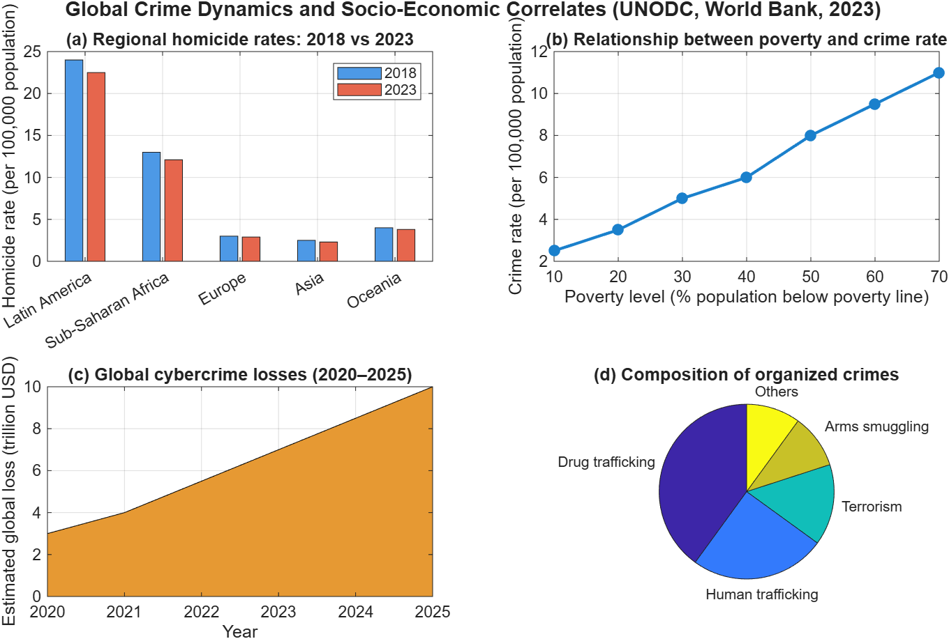
Empirical data underscore the pressing nature of crime as a global issue. The United Nations Office on Drugs and Crime (UNODC) reported that the global homicide rate in 2018 was approximately 6.1 per 100,000 population, though this figure varies significantly across regions. Many urban centers in Latin America and sub-Saharan Africa record homicide rates far higher than the global average, whereas Europe and Asia exhibit considerably lower rates. The 2023 UNODC Global Report further estimates the worldwide homicide rate at about 5.8 per 100,000 population, confirming persistent regional disparities. In addition, economic indicators from the World Bank demonstrate that countries with high levels of poverty and income inequality tend to experience elevated crime rates. Conversely, nations with stronger governance structures and better education systems generally report lower incidences of crime. Moreover, the rapid expansion of technology has contributed to an alarming surge in cybercrime, with global losses projected to exceed $10 trillion by 2025, according to Cybersecurity Ventures. Organized criminal activities such as drug trafficking, human trafficking, and terrorism-related offenses also remain major challenges for international law enforcement agencies. Overall, these global patterns reveal a strong correlation between socio-economic disparities and criminal activity, highlighting both shared and contrasting trends when compared with the Indian context. They emphasize the critical need for robust, data-driven mathematical models capable of capturing these complex interrelations and guiding the formulation of effective crime prevention and intervention strategies (see Figure 2).
Mathematical modeling of criminal behavior has become an important research avenue for understanding the mechanisms that govern the rise, persistence, and control of crime. Early conceptual frameworks, notably the Crime Pattern Theory proposed by Brantingham and Brantingham [1], emphasized spatial and situational factors shaping the geography of offenses. Building upon this foundation, Short et al. [2] developed reaction–diffusion models that integrate offender decision-making, repeat victimization, and environmental feedbacks. Their work demonstrated how localized interactions among offenders, targets, and deterrents can lead to the spontaneous formation of crime “hotspots,” revealing the self-organizing nature of criminal activity.
Further advances were made by Berestycki and Nadal [3], who analyzed the existence, stability, and bifurcation of steady-state crime distributions. These studies showed that nonlinear reinforcement mechanisms, such as imitation and deterrence, can generate multiple equilibria and sharp transitions between low- and high-crime regimes, features characteristic of complex adaptive systems. Collectively, this body of work highlights that crime propagation is governed by nonlinear interactions, feedback loops, and sensitivity to environmental and social parameters.
Recent developments in nonlinear dynamical systems theory have further expanded the scope of crime modeling from spatially distributed frameworks to compartmental population-based systems [4]. Such models divide the population into behavioral categories—law-abiding, at-risk, active offenders, and rehabilitated individuals—and describe transitions between them via parameters representing recruitment, deterrence, and social rehabilitation. Nonlinear feedbacks such as social pressure or peer imitation can induce threshold effects, multistability, and bifurcation phenomena demonstrating how small policy or behavioral changes can yield abrupt shifts between equilibrium states.
Habitual criminals constitute a distinct and influential subgroup within the broader spectrum of offenders. Unlike first-time or opportunistic offenders, habitual criminals exhibit repeated engagement in unlawful activities and display limited responsiveness to traditional deterrence or rehabilitation measures. Empirical studies and criminological observations suggest that such individuals often serve as catalysts for sustaining criminal networks, influencing at-risk individuals through imitation, social reinforcement, and normalization of deviant behavior. From a modeling perspective, incorporating a separate compartment for habitual offenders (\(\mathcal{H}\)) allows for the explicit representation of this feedback mechanism, capturing the persistence and self-propagating nature of crime in a community. This distinction is crucial for understanding why crime may persist even when preventive or corrective interventions are active. By quantifying the rate at which active criminals transition into habitual offenders (\(\eta\)) and the corresponding rate of their removal or rehabilitation (\(\rho\)), the model provides a means to evaluate the long-term societal impact of repeat offenses. Furthermore, analyzing how habitual offenders influence the basic reproduction number (\(\mathcal{R}_c\)) offers valuable insights into thresholds of stability and the effectiveness of targeted policies aimed at breaking cycles of recidivism. Thus, the inclusion of the \(\mathcal{H}\) compartment enhances the model’s realism and its relevance for designing sustainable crime-control strategies.
To capture the evolution of crime considering imitation effects among individuals, we propose a nonlinear system of ordinary differential equations that divides the total population into five interacting compartments:
\(S_1\) (individuals not at risk),
\(S_2\) (individuals at risk),
\(C\) (active criminals),
\(H\) (habitual offenders, less receptive to rehabilitation), and
\(R\) (convicted or rehabilitated individuals).
The model is governed by the following system: \[ \frac{dS_1}{dt} = (1-p)\pi + (1 – q)\gamma R – (\mu+\theta)S_1 + \epsilon S_2, \label{eq:s1}\ \tag{1}\] \[\frac{dS_2}{dt} = p\pi – \beta S_2C(1+\alpha C) – (\mu+\epsilon)S_2 + \theta S_1, \label{eq:s2}\ \tag{2}\] \[\frac{dC}{dt} = \beta S_2C(1+\alpha C) + q\gamma R – (\mu+\sigma+\eta)C, \label{eq:c}\ \tag{3}\] \[\frac{dH}{dt} = \eta C – (\mu + \rho)H, \label{eq:h}\ \tag{4}\] \[\frac{dR}{dt} = \sigma C + \rho H – (\mu+\gamma)R. \label{eq:r} \tag{5}\]
Here, \(\pi\) is the recruitment rate of new individuals; \(p\) is the fraction entering the at-risk group; \(q\) denotes the fraction of convicted individuals returning to crime; \(\beta\) is the crime initiation rate; \(\alpha\) captures the influence of rising criminal activity; \(\gamma\) is the rehabilitation rate; \(\sigma\), \(\eta\), and \(\rho\) represent conviction, habituation, and arrest rates, respectively; \(\mu\) is the natural exit rate; \(\theta\) is the transition rate to the at-risk group; and \(\epsilon\) represents the reverse transition to the non-risk group.
Let \(N(t) = S_1 + S_2 + C + H + R\) be the total population. Summing Eqs. (1)–(5) yields: \[\frac{dN}{dt} = \pi – \mu N. \label{eq:N} \tag{6}\]
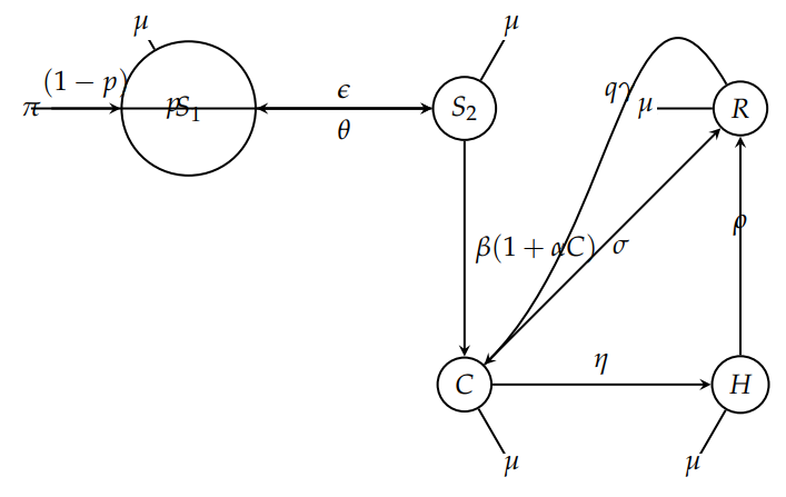
Eq. (6) shows that the total population grows through constant recruitment (\(\pi\)) and declines at a natural rate (\(\mu\)). It also reflects that criminal entry and exit occur within this dynamic balance. State transition diagram showing the flow between compartments in the crime model is given in Figure 3.
Theorem 1(Positivity and Boundedness of Solutions).Let the initial condition be \[\mathbf{X}(0) = \big(S_1(0),\, S_2(0),\, C(0),\, H(0),\, R(0)\big)^\top \in \mathbb{R}_+^5 = \{ (x_1,\dots,x_5)\in\mathbb{R}^5 : x_i > 0 \ \forall i\}.\]
Then, the solution \[\mathbf{X}(t) = \big(S_1(t),\, S_2(t),\, C(t),\, H(t),\, R(t)\big)^\top,\] of system (1)–(5) remains positive and bounded for all \(t \geq 0\). Moreover, there exists a compact positively invariant set \[\Omega = \left\{ (S_1,S_2,C,H,R) \in \mathbb{R}_+^5 : N(t) = S_1 + S_2 + C + H + R \leq \frac{\pi}{\mu} \right\},\] such that every trajectory of the system that begins in \(\Omega\) remains in \(\Omega\) for all future time.
Proof. Local existence and uniqueness follow from the right-hand sides being locally Lipschitz. It remains to show positivity and boundedness.
Let the initial data satisfy \(S_1(0),S_2(0),C(0),H(0),R(0)>0\). Each equation can be written in the form \[\dot{x}(t)+a(t)x(t)=b(t),\] with \(a(t)\ge 0\) and \(b(t)\ge 0\) for the corresponding component. Hence, by the integrating-factor (variation-of-constants) formula, \[x(t)=x(0)e^{-\int_0^t a(s)\,ds}+\int_0^t e^{-\int_s^t a(u)\,du}\,b(s)\,ds \ge x(0)e^{-\int_0^t a(s)\,ds}>0,\] for all \(t\ge0\). Applying this argument componentwise yields \[S_1(t)\ge S_1(0)e^{-(\mu+\theta)t},\quad S_2(t)\ge S_2(0)e^{-\int_0^t a_{S_2}(s)\,ds},\quad C(t)\ge C(0)e^{-(\mu+\sigma+\eta)t},\] and analogous positive lower bounds for \(H(t)\) and \(R(t)\). Thus no component can vanish or become negative for \(t\ge0\).
(Equivalently, a boundary contradiction argument shows that if any component attained zero at some \(t^*>0\) then its derivative at \(t^*\) would be nonnegative—indeed strictly positive under mild parameter conditions—preventing crossing into the negative half-line.) ◻
Theorem 2(Boundedness and Positively Invariant Region). Consider the system (1)–(5) with the initial condition \[\mathbf{X}(0) = \big(S_1(0),\, S_2(0),\, C(0),\, H(0),\, R(0)\big)^\top \in \mathbb{R}_+^5.\]
Let the total population be \[N(t) = S_1(t) + S_2(t) + C(t) + H(t) + R(t).\]
Then, the solution \(\mathbf{X}(t)\) of the system satisfies \[0 \le S_i(t) \le M, \qquad i = 1,2,3,4,5, \quad \forall\, t \ge 0,\] where \[M := \max\!\left\{ N(0),\, \frac{\pi}{\mu} \right\}.\]
Consequently, all system trajectories enter and remain in the compact, positively invariant set \[\Omega = \left\{ (S_1,S_2,C,H,R)\in\mathbb{R}_+^5 : S_1+S_2+C+H+R \le \frac{\pi}{\mu} \right\}.\]
Moreover, \(\Omega\) is globally attracting; that is, for any initial condition in \(\mathbb{R}_+^5\), \[\lim_{t\to\infty} N(t) = \frac{\pi}{\mu}.\]
Proof. Summing Eqs. (1)–(5) yields \[\frac{dN}{dt} = \pi – \mu N(t),\] whose solution is \[N(t) = N(0)e^{-\mu t} + \frac{\pi}{\mu}\big(1 – e^{-\mu t}\big).\]
It follows that \[\min\!\left\{N(0),\,\frac{\pi}{\mu}\right\} \le N(t) \le \max\!\left\{N(0),\,\frac{\pi}{\mu}\right\}, \qquad \forall\, t \ge 0.\]
Hence, each component satisfies \[0 \le S_i(t),\, C(t),\, H(t),\, R(t) \le M := \max\!\left\{N(0),\,\frac{\pi}{\mu}\right\}, \qquad \forall\, t \ge 0.\]
If \(N(0)\le \pi/\mu\), then \(N(t)\le \pi/\mu\) for all \(t\ge0\), so every trajectory remains inside the feasible region \[\Omega = \big\{(S_1,S_2,C,H,R)\in\mathbb{R}_+^5:\, N(t)\le \tfrac{\pi}{\mu}\big\}.\]
If \(N(0)>\pi/\mu\), then \(N(t)\) decreases monotonically to \(\pi/\mu\) as \(t\to\infty\), proving that \(\Omega\) is positively invariant and globally attracting. ◻
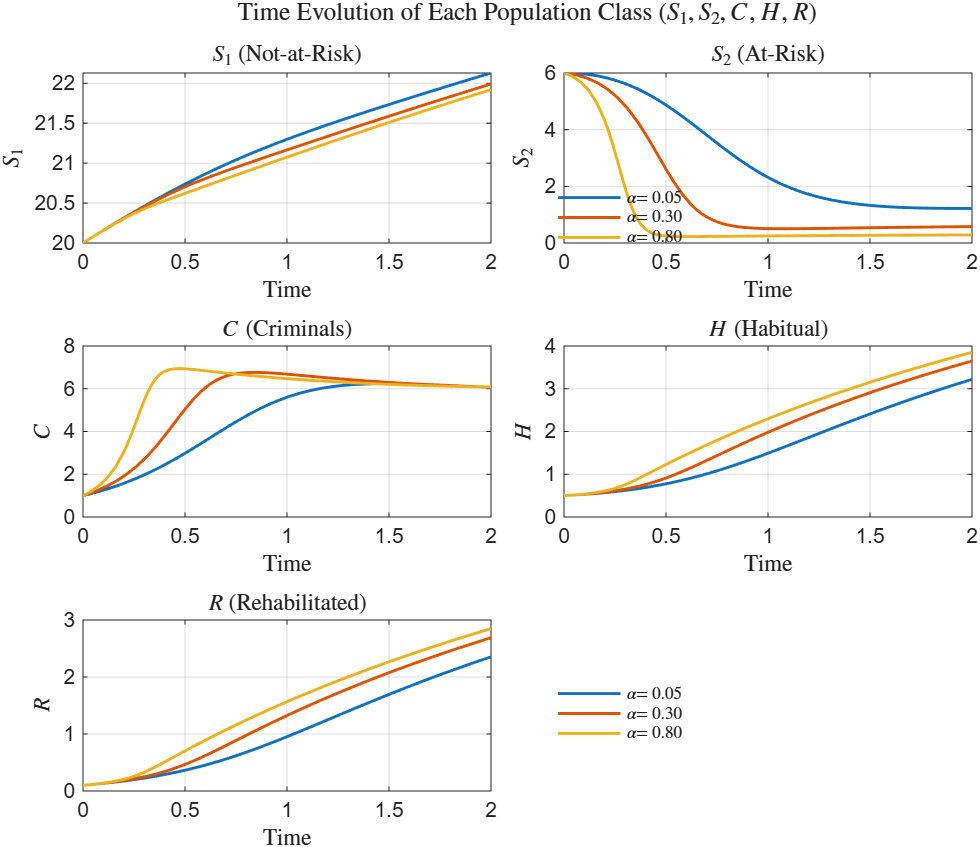
Figure 4 depicts the temporal evolution of the five population classes—\(\mathcal{S}_1\) (Not-at-Risk), \(\mathcal{S}_2\) (At-Risk), \(\mathcal{C}\) (Criminals), \(\mathcal{H}\) (Habitual), and \(\mathcal{R}\) (Rehabilitated)—for varying values of the behavioral parameter \(\alpha = 0.05, 0.30, 0.80\), which characterizes the non-linear influence of criminals on at-risk individuals. The simulations, conducted over \(t \in [0, 2]\), capture the transient behavior of the system, with all state variables approaching steady levels beyond \(t \approx 1.5\). As \(\alpha\) increases, the criminal population (\(\mathcal{C}\)) rises more rapidly, the at-risk class (\(\mathcal{S}_2\)) declines sharply, and both habitual offenders (\(\mathcal{H}\)) and rehabilitated individuals (\(\mathcal{R}\)) grow faster, while the not-at-risk group (\(\mathcal{S}_1\)) exhibits only a mild increase. These patterns underscore the amplifying role of higher \(\alpha\) in driving the conversion of at-risk individuals into active criminals, thereby influencing the overall population redistribution within the system.
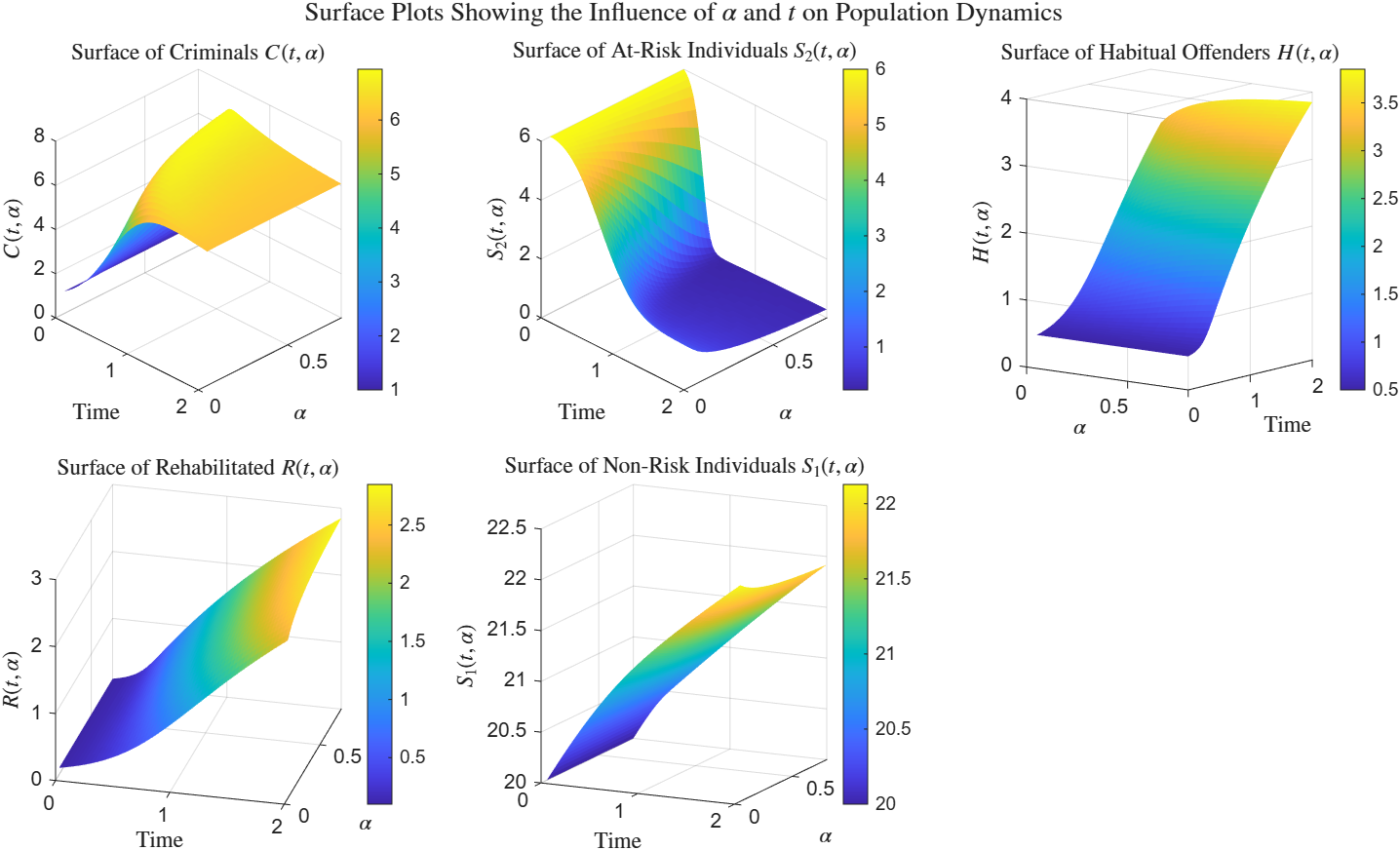
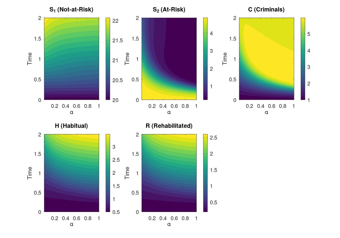
Figure 5 presents the surface plots of the five key population compartments—\(\mathcal{S}_1\) (Not-at-Risk), \(\mathcal{S}_2\) (At-Risk), \(\mathcal{C}\) (Criminals), \(\mathcal{H}\) (Habitual), and \(\mathcal{R}\) (Rehabilitated)—as functions of both time (\(t\)) and the imitation rate (\(\alpha\)). The three-dimensional representations provide a clear visualization of how temporal evolution interacts with behavioral intensity to shape population transitions. As \(\alpha\) increases, the surface of \(\mathcal{C}(t,\alpha)\) rises sharply, indicating accelerated recruitment into criminal activity, while \(\mathcal{S}_2(t,\alpha)\) declines significantly, reflecting depletion of the at-risk group. Conversely, \(\mathcal{H}(t,\alpha)\) and \(\mathcal{R}(t,\alpha)\) exhibit positive growth surfaces, implying that higher imitation strength promotes habitual offending and rehabilitation. The surface of \(\mathcal{S}_1(t,\alpha)\) shows only a mild upward trend, consistent with the gradual stabilization of the non-risk population. These results collectively demonstrate that the imitation parameter \(\alpha\) acts as a key driver in the propagation and stabilization of criminal dynamics over time.
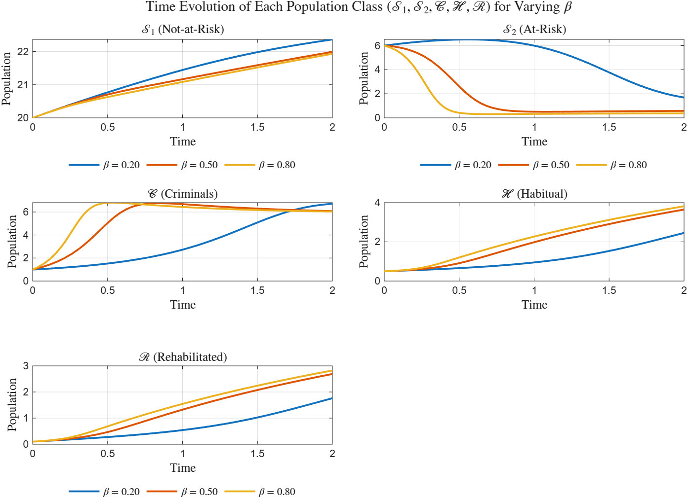
To examine the influence of the crime initiation rate (\(\beta\)) on the population dynamics, the system was simulated for three representative values, \(\beta = 0.20,\, 0.50,\, 0.80\), while keeping all other parameters fixed. The results, shown in Figure 6, illustrate the temporal evolution of the five interacting compartments—\(\mathcal{S}_1\) (Not-at-Risk), \(\mathcal{S}_2\) (At-Risk), \(\mathcal{C}\) (Criminals), \(\mathcal{H}\) (Habitual), and \(\mathcal{R}\) (Rehabilitated). The simulations were performed over \(t \in [0, 2]\), which adequately captures the transient and stabilization phases of each subpopulation.
As observed from Figure 6, higher values of \(\beta\) substantially accelerate the transition of at-risk individuals (\(\mathcal{S}_2\)) into the criminal class (\(\mathcal{C}\)). This increase in \(\beta\) enhances the rate of criminal recruitment, causing a rapid depletion of the at-risk population and a corresponding rise in both habitual offenders (\(\mathcal{H}\)) and rehabilitated individuals (\(\mathcal{R}\)). The not-at-risk group (\(\mathcal{S}_1\)) exhibits only a marginal change, reflecting its relatively weak sensitivity to variations in \(\beta\). Notably, for \(\beta = 0.80\), the criminal population reaches its saturation much earlier, indicating a faster approach toward a quasi-equilibrium state. These dynamics confirm that \(\beta\) serves as a critical driver of short-term crime escalation and the subsequent redistribution of individuals across the population compartments.
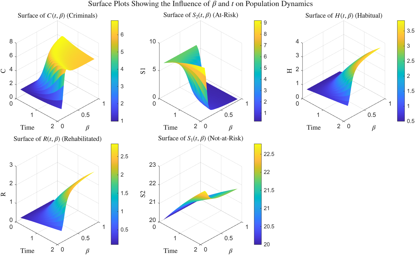
The three-dimensional surfaces in Figure 7 provide further insight into the coupled effects of \(\beta\) and time (\(t\)) on each subpopulation. The surface \(\mathcal{C}(t,\beta)\) shows a pronounced upward curvature with increasing \(\beta\), emphasizing the nonlinear amplification of criminal activity as crime initiation intensifies. Conversely, the surface \(\mathcal{S}_2(t,\beta)\) declines steeply with higher \(\beta\), signifying the rapid depletion of at-risk individuals. The surfaces for \(\mathcal{H}(t,\beta)\) and \(\mathcal{R}(t,\beta)\) exhibit monotonic growth patterns, demonstrating that elevated \(\beta\) values increase both habitual offending and rehabilitation transitions. In contrast, \(\mathcal{S}_1(t,\beta)\) remains relatively stable across all \(\beta\) values, consistent with its slower interaction rate in the model. Overall, these results indicate that an increase in \(\beta\) enhances the nonlinear coupling between at-risk and criminal populations, driving the system toward a faster but more imbalanced steady state dominated by criminal and habitual classes.
To explore the combined influence of the crime initiation rate (\(\beta\)) and the rehabilitation rate (\(\gamma\)) on the population dynamics, we numerically solved the model over \(t \in [0,2]\) and evaluated the population levels at \(t = 1.5\), corresponding to the near steady-state regime. Figure 8 presents the one-dimensional variation of each subpopulation with respect to \(\beta\) for three representative values of \(\gamma = 0.1,\,0.4,\,0.8\), while Figure 9 shows the two-dimensional surface plots illustrating the joint effects of \(\beta\) and \(\gamma\) on all five compartments: \(\mathcal{S}_1\) (Not-at-Risk), \(\mathcal{S}_2\) (At-Risk), \(\mathcal{C}\) (Criminals), \(\mathcal{H}\) (Habitual), and \(\mathcal{R}\) (Rehabilitated).
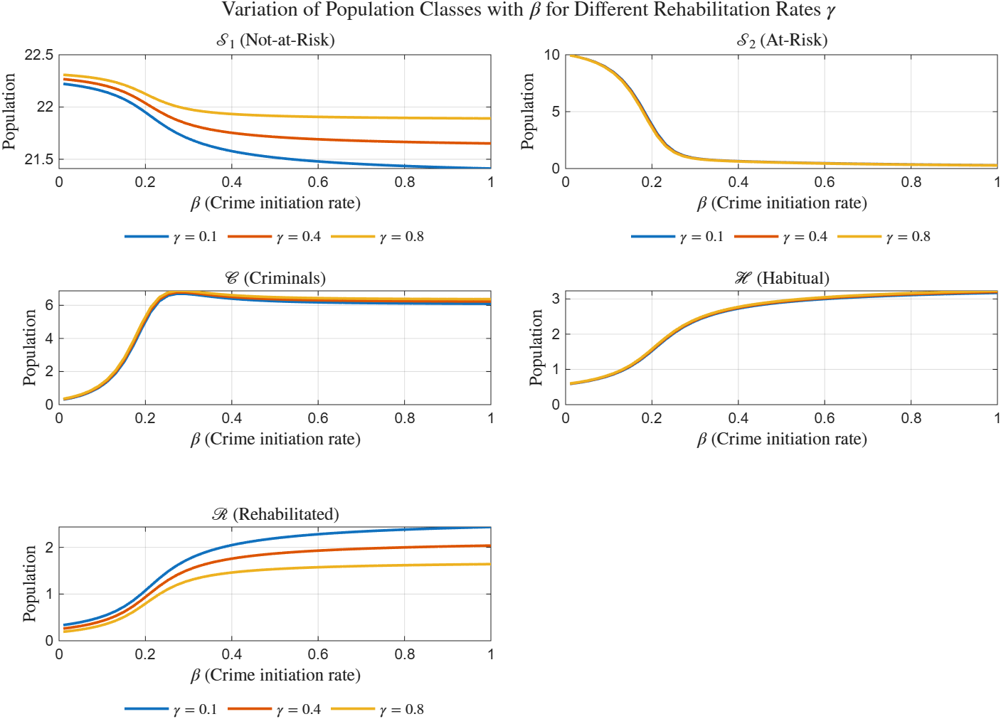
As shown in Figure 8, an increase in \(\beta\) results in a strong nonlinear response in the criminal population (\(\mathcal{C}\)), which rapidly rises to a peak before stabilizing as the at-risk group (\(\mathcal{S}_2\)) becomes depleted. This trend is particularly pronounced at lower rehabilitation rates (\(\gamma\)), where criminal recruitment dominates the system dynamics. Conversely, higher values of \(\gamma\) effectively suppress criminal activity by accelerating the rehabilitation process, leading to a larger proportion of individuals in the rehabilitated compartment (\(\mathcal{R}\)). The habitual offenders (\(\mathcal{H}\)) exhibit a moderate increase with \(\beta\), while the not-at-risk population (\(\mathcal{S}_1\)) remains relatively stable across all parameter ranges. These results emphasize the opposing regulatory effects of \(\beta\) and \(\gamma\): while \(\beta\) drives the amplification of crime through recruitment mechanisms, \(\gamma\) mitigates it by enhancing the reintegration of convicted individuals into society.
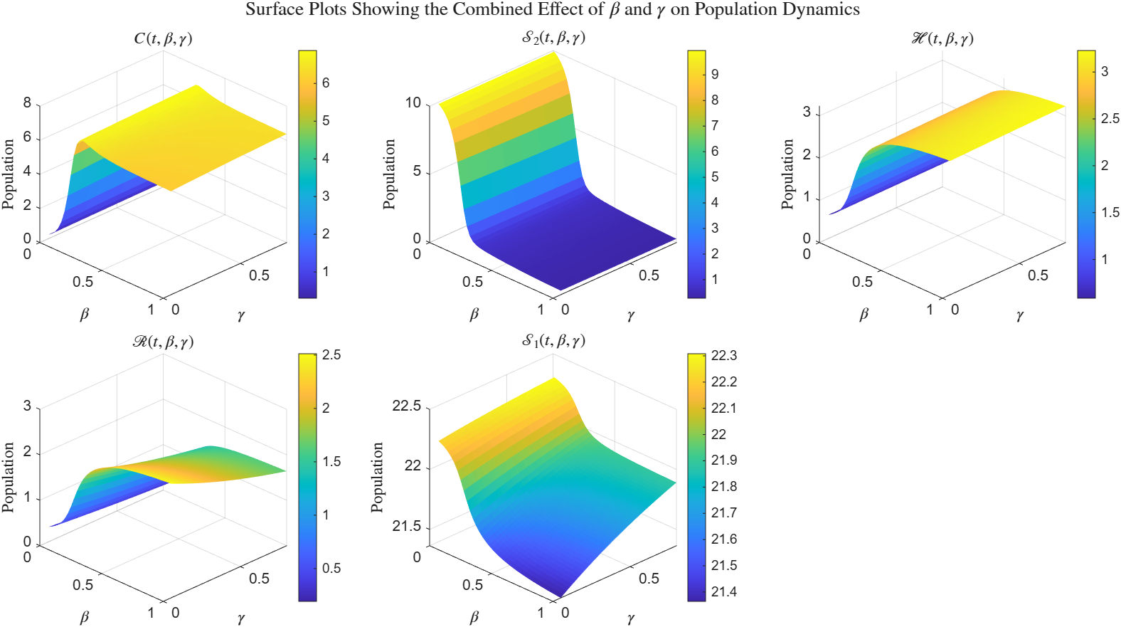
The surface plots in Figure 9 provide a more comprehensive view of the \(\beta\)–\(\gamma\) interaction. The surface \(\mathcal{C}(t,\beta,\gamma)\) displays a sharp ridge along low \(\gamma\) values and moderate \(\beta\), representing a high-crime regime. As \(\gamma\) increases, this ridge flattens, indicating that efficient rehabilitation significantly reduces criminal prevalence. The surface \(\mathcal{S}_2(t,\beta,\gamma)\) exhibits a complementary decline pattern, showing rapid depletion of at-risk individuals as \(\beta\) increases. Meanwhile, \(\mathcal{H}(t,\beta,\gamma)\) and \(\mathcal{R}(t,\beta,\gamma)\) surfaces exhibit monotonic growth with \(\beta\) and \(\gamma\), signifying increased transitions into habitual offending and successful rehabilitation. The not-at-risk class \(\mathcal{S}_1(t,\beta,\gamma)\) remains largely unaffected, maintaining near-constant population levels. Overall, these results demonstrate that the interplay between \(\beta\) and \(\gamma\) governs the long-term balance between crime proliferation and rehabilitation, where enhancing \(\gamma\) can effectively offset the destabilizing influence of high \(\beta\), guiding the system toward a socially stable equilibrium.
In the context of nonlinear dynamical systems, equilibrium points represent the steady states at which the time evolution of all system variables ceases. For the proposed crime dynamics model (9), these equilibria correspond to long-term distributions of the population across the compartments \(\mathcal{S}_1\), \(\mathcal{S}_2\), \(\mathcal{C}\), \(\mathcal{H}\), and \(\mathcal{R}\).
Definition 1(Equilibrium Points).Let \( {\mathcal{X}}(t) = (\mathcal{S}_1(t), \mathcal{S}_2(t), \mathcal{C}(t), \mathcal{H}(t), \mathcal{R}(t))^\top\) be a solution of system (9). A point \(\bar{ {\mathcal{X}}} = (\bar{\mathcal{S}}_1, \bar{\mathcal{S}}_2, \bar{\mathcal{C}}, \bar{\mathcal{H}}, \bar{\mathcal{R}})^\top \in \Omega\) is called an equilibrium point if \[ {\mathcal{F}}(\bar{ {\mathcal{X}}}) = {0}.\]
Three types of equilibria are possible:
Trivial equilibrium: the zero state \(\bar{ {\mathcal{X}}} = {0}\) (no population), which is biologically irrelevant and excluded from the feasible region \(\Omega\)
Crime-free equilibrium (CFE): the state in which no active or habitual criminals exist, i.e., \(\bar{\mathcal{C}} = \bar{\mathcal{H}} = 0\), while \(\bar{\mathcal{S}}_1\), \(\bar{\mathcal{S}}_2\), and \(\bar{\mathcal{R}}\) remain positive.
Endemic (crime-persistent) equilibrium: a steady state with \(\bar{\mathcal{C}} > 0\), \(\bar{\mathcal{H}} > 0\), corresponding to persistent criminal activity in the population.
The existence and stability of these equilibria determine whether crime will die out or persist in the long run [5].
The model (9) can be rewritten compactly in vector form as: \[\frac{d {\mathcal{X}}}{dt} = \mathbf{A} {\mathcal{X}} + \mathbf{B} + \mathbf{G}( {\mathcal{X}}),\] where \(\mathbf{A}\) contains the linear transition terms, \(\mathbf{B}\) represents constant recruitment, and \(\mathbf{G}( {\mathcal{X}})\) includes the nonlinear imitation and recruitment effects associated with criminal behavior: \[\mathbf{A} = \begin{bmatrix} -(\mu+\theta) & \epsilon & 0 & 0 & (1-q)\gamma \\ \theta & -(\mu+\epsilon) & 0 & 0 & 0 \\ 0 & 0 & -(\mu+\sigma+\eta) & 0 & q\gamma \\ 0 & 0 & \eta & -(\mu+\rho) & 0 \\ 0 & 0 & \sigma & \rho & -(\mu+\gamma) \end{bmatrix}, \quad \mathbf{B} = \begin{bmatrix} (1-p)\pi \\[4pt] p\pi \\[4pt] 0 \\[4pt] 0 \\[4pt] 0 \end{bmatrix},\] \[\mathbf{G}( {\mathcal{X}}) = \begin{bmatrix} 0 \\[4pt] -\beta \mathcal{S}_2\mathcal{C}(1+\alpha \mathcal{C}) \\[4pt] \beta \mathcal{S}_2\mathcal{C}(1+\alpha \mathcal{C}) \\[4pt] 0 \\[4pt] 0 \end{bmatrix}.\]
A steady state \(\bar{ {\mathcal{X}}}\) therefore satisfies: \[ {0} = \mathbf{A}\bar{ {\mathcal{X}}} + \mathbf{B} + \mathbf{G}(\bar{ {\mathcal{X}}}),\] which yields the algebraic system: \[ (1-p)\pi + (1-q)\gamma \bar{\mathcal{R}} – (\mu+\theta)\bar{\mathcal{S}}_1 + \epsilon \bar{\mathcal{S}}_2 = 0, \label{eq:eq1}\ \tag{7a}\] \[p\pi – \beta \bar{\mathcal{S}}_2\bar{\mathcal{C}}(1+\alpha \bar{\mathcal{C}}) – (\mu+\epsilon)\bar{\mathcal{S}}_2 + \theta \bar{\mathcal{S}}_1 = 0, \label{eq:eq2}\ \tag{7b}\] \[\beta \bar{\mathcal{S}}_2\bar{\mathcal{C}}(1+\alpha \bar{\mathcal{C}}) + q\gamma \bar{\mathcal{R}} – (\mu+\sigma+\eta)\bar{\mathcal{C}} = 0, \label{eq:eq3}\ \tag{7c}\] \[\eta \bar{\mathcal{C}} – (\mu + \rho)\bar{\mathcal{H}} = 0, \label{eq:eq4}\ \tag{7d}\] \[\sigma \bar{\mathcal{C}} + \rho \bar{\mathcal{H}} – (\mu+\gamma)\bar{\mathcal{R}} = 0, \label{eq:eq5}\ \tag{7e}\] \[\bar{\mathcal{S}}_1 + \bar{\mathcal{S}}_2 + \bar{\mathcal{C}} + \bar{\mathcal{H}} + \bar{\mathcal{R}} = \frac{\pi}{\mu}. \label{eq:eq6} \tag{7f}\]
Setting \(\bar{\mathcal{C}} = \bar{\mathcal{H}} = 0\) in (7), we obtain the crime-free equilibrium \[E_0 = (\bar{\mathcal{S}}_1^0, \bar{\mathcal{S}}_2^0, 0, 0, \bar{\mathcal{R}}^0),\] where \[\bar{\mathcal{S}}_1^0 = \frac{(1-p)\pi + (1-q)\gamma \bar{\mathcal{R}}^0 + \epsilon \bar{\mathcal{S}}_2^0}{\mu+\theta}, \qquad \bar{\mathcal{S}}_2^0 = \frac{p\pi + \theta \bar{\mathcal{S}}_1^0}{\mu+\epsilon}, \qquad \bar{\mathcal{R}}^0 = 0.\]
This equilibrium represents a crime-free society in which only the non-criminal classes remain. The local stability of \(E_0\) is determined by the basic reproduction number \(R_c\), which acts as a threshold between crime eradication and persistence [5].
When \(\bar{\mathcal{C}} > 0\), the nonlinear term \(\mathbf{G}( {\mathcal{X}})\) becomes active, leading to the endemic (crime-persistent) equilibrium. Solving (7a)–(7f) by expressing \(\bar{\mathcal{S}}_1\), \(\bar{\mathcal{S}}_2\), \(\bar{\mathcal{H}}\), and \(\bar{\mathcal{R}}\) in terms of \(\bar{\mathcal{C}}\) gives: \[\bar{\mathcal{H}}^* = \frac{\eta}{\mu+\rho}\,\bar{\mathcal{C}}^*, \qquad \bar{\mathcal{R}}^* = \frac{1}{\mu+\gamma}\Big(\sigma+\tfrac{\rho\eta}{\mu+\rho}\Big)\bar{\mathcal{C}}^*,\] \[\bar{\mathcal{S}}_2^* = \frac{(\mu+\sigma+\eta)(\mu+\gamma)(\mu+\rho) – q\gamma\big[\sigma(\mu+\rho)+\rho\eta\big]}% {\beta(1+\alpha \bar{\mathcal{C}}^*)(\mu+\gamma)(\mu+\rho)},\] \[\begin{aligned} \bar{\mathcal{S}}_1^* =& \frac{\beta(1+\alpha \bar{\mathcal{C}}^*)(\mu+\gamma)(\mu+\rho)(1-p)\pi + \beta(1+\alpha \bar{\mathcal{C}}^*)(1-q)\gamma[\sigma(\mu+\rho)+\rho\eta]\bar{\mathcal{C}}^* } {(\mu+\theta)\,\beta(1+\alpha \bar{\mathcal{C}}^*)(\mu+\gamma)(\mu+\rho)}\\&+\frac{\epsilon[(\mu+\sigma+\eta)(\mu+\gamma)(\mu+\rho) – q\gamma(\sigma(\mu+\rho)+\rho\eta)]} {(\mu+\theta)\,\beta(1+\alpha \bar{\mathcal{C}}^*)(\mu+\gamma)(\mu+\rho)}. \end{aligned}\]
Substituting these into (7f) and simplifying leads to the quadratic relation \[k_1(\bar{\mathcal{C}}^*)^2 + k_2\bar{\mathcal{C}}^* + k_3 = 0,\] where the coefficients \(k_1\), \(k_2\), and \(k_3\) depend on model parameters as derived earlier. The positive real roots of this equation correspond to biologically admissible endemic equilibria.
In accordance with Lemma 1, these equilibria occur at the intersection of the nullclines \(\mathcal{N}_{\mathcal{C}}\) and \(\mathcal{N}_{\mathcal{S}_2}\) within the feasible region \(\Omega\). The persistence of this equilibrium when \(R_c>1\) follows from Lemma 2.
To investigate the relative influence of parameters on the endemic steady state \((\bar{\mathcal{S}}_1^*, \bar{\mathcal{S}}_2^*, \bar{\mathcal{C}}^*, \bar{\mathcal{H}}^*, \bar{\mathcal{R}}^*)\), each parameter is perturbed by \(\{-20\%, -10\%, 0, +10\%, +20\}\) around its baseline value, while others are held constant. The resulting variations in the equilibrium values are computed numerically and summarized in Table 1. This analysis identifies the parameters with the greatest sensitivity, thereby highlighting effective intervention targets for crime prevention policies [5, 6].
| Parameter | Change | \(S_1^*\) | \(S_2^*\) | \(C^*\) | \(H^*\) | \(R^*\) |
|---|---|---|---|---|---|---|
| \(\pi\) | -20% | 27.887 | 0.934 | 21.934 | 9.400 | 19.845 |
| -10% | 31.358 | 0.875 | 24.757 | 10.610 | 22.399 | |
| +0% | 34.829 | 0.823 | 27.578 | 11.819 | 24.951 | |
| +10% | 38.301 | 0.777 | 30.395 | 13.026 | 27.500 | |
| +20% | 41.773 | 0.736 | 33.210 | 14.233 | 30.047 | |
| \(\mu\) | -20% | 42.121 | 0.669 | 34.020 | 15.464 | 32.726 |
| -10% | 38.083 | 0.747 | 30.452 | 13.435 | 28.396 | |
| +0% | 34.829 | 0.823 | 27.578 | 11.819 | 24.951 | |
| +10% | 32.148 | 0.899 | 25.209 | 10.504 | 22.149 | |
| +20% | 29.898 | 0.973 | 23.220 | 9.414 | 19.829 | |
| \(\sigma\) | -20% | 33.661 | 0.712 | 29.830 | 12.784 | 23.012 |
| -10% | 34.268 | 0.767 | 28.661 | 12.283 | 24.021 | |
| +0% | 34.829 | 0.823 | 27.578 | 11.819 | 24.951 | |
| +10% | 35.350 | 0.880 | 26.571 | 11.387 | 25.811 | |
| +20% | 35.835 | 0.939 | 25.632 | 10.985 | 26.609 | |
| \(\eta\) | -20% | 34.880 | 0.751 | 29.259 | 10.032 | 25.079 |
| -10% | 34.854 | 0.787 | 28.394 | 10.952 | 25.014 | |
| +0% | 34.829 | 0.823 | 27.578 | 11.819 | 24.951 | |
| +10% | 34.806 | 0.860 | 26.806 | 12.637 | 24.891 | |
| +20% | 34.785 | 0.897 | 26.075 | 13.410 | 24.833 | |
| \(p\) | -20% | 37.005 | 0.840 | 26.638 | 11.416 | 24.101 |
| -10% | 35.917 | 0.831 | 27.108 | 11.618 | 24.526 | |
| +0% | 34.829 | 0.823 | 27.578 | 11.819 | 24.951 | |
| +10% | 33.741 | 0.815 | 28.047 | 12.020 | 25.376 | |
| +20% | 32.653 | 0.807 | 28.517 | 12.222 | 25.801 | |
| \(q\) | -20% | 37.123 | 0.909 | 26.558 | 11.382 | 24.028 |
| -10% | 35.998 | 0.866 | 27.058 | 11.596 | 24.481 | |
| +0% | 34.829 | 0.823 | 27.578 | 11.819 | 24.951 | |
| +10% | 33.615 | 0.781 | 28.116 | 12.050 | 25.438 | |
| +20% | 32.353 | 0.740 | 28.674 | 12.289 | 25.943 | |
| \(\alpha\) | -20% | 34.839 | 0.932 | 27.527 | 11.797 | 24.905 |
| -10% | 34.834 | 0.874 | 27.554 | 11.809 | 24.930 | |
| +0% | 34.829 | 0.823 | 27.578 | 11.819 | 24.951 | |
| +10% | 34.825 | 0.778 | 27.599 | 11.828 | 24.970 | |
| +20% | 34.822 | 0.737 | 27.618 | 11.836 | 24.987 | |
| \(\theta\) | -20% | 39.082 | 0.856 | 25.741 | 11.032 | 23.289 |
| -10% | 36.833 | 0.838 | 26.712 | 11.448 | 24.168 | |
| +0% | 34.829 | 0.823 | 27.578 | 11.819 | 24.951 | |
| +10% | 33.032 | 0.810 | 28.353 | 12.151 | 25.653 | |
| +20% | 31.411 | 0.798 | 29.053 | 12.451 | 26.286 | |
| \(\rho\) | -20% | 34.347 | 0.837 | 27.132 | 13.566 | 24.117 |
| -10% | 34.605 | 0.830 | 27.370 | 12.632 | 24.563 | |
| +0% | 34.829 | 0.823 | 27.578 | 11.819 | 24.951 | |
| +10% | 35.026 | 0.818 | 27.760 | 11.104 | 25.292 | |
| +20% | 35.201 | 0.813 | 27.921 | 10.470 | 25.594 | |
| \(\gamma\) | -20% | 33.429 | 0.864 | 26.283 | 11.264 | 28.160 |
| -10% | 34.172 | 0.842 | 26.969 | 11.558 | 26.459 | |
| +0% | 34.829 | 0.823 | 27.578 | 11.819 | 24.951 | |
| +10% | 35.416 | 0.807 | 28.120 | 12.051 | 23.606 | |
| +20% | 35.943 | 0.793 | 28.606 | 12.260 | 22.398 | |
| \(\epsilon\) | -20% | 34.784 | 0.823 | 27.597 | 11.827 | 24.969 |
| -10% | 34.807 | 0.823 | 27.587 | 11.823 | 24.960 | |
| +0% | 34.829 | 0.823 | 27.578 | 11.819 | 24.951 | |
| +10% | 34.852 | 0.823 | 27.568 | 11.815 | 24.942 | |
| +20% | 34.874 | 0.824 | 27.558 | 11.811 | 24.934 | |
| \(\beta\) | -20% | 34.847 | 1.031 | 27.481 | 11.777 | 24.863 |
| -10% | 34.837 | 0.916 | 27.535 | 11.801 | 24.912 | |
| +0% | 34.829 | 0.823 | 27.578 | 11.819 | 24.951 | |
| +10% | 34.823 | 0.748 | 27.613 | 11.834 | 24.983 | |
| +20% | 34.817 | 0.685 | 27.642 | 11.847 | 25.009 |
We conducted a sensitivity analysis to examine how changes in model parameters affect the endemic equilibrium values. The baseline parameter values used in our MATLAB simulations are given in Table 2.
| Parameter | Baseline Value |
|---|---|
| \(\pi\) (Recruitment rate) | 1000 |
| \(\mu\) (Natural death rate) | 0.02 |
| \(\sigma\) (Conviction rate) | 0.1 |
| \(\eta\) (Habitual criminal rate) | 0.05 |
| \(p\) (At-risk fraction) | 0.3 |
| \(q\) (Recidivism fraction) | 0.4 |
| \(\alpha\) (Crime enhancement) | 0.001 |
| \(\theta\) (Rehabilitation rate) | 0.1 |
| \(\rho\) (Arrest rate) | 0.15 |
| \(\gamma\) (Rehabilitation rate) | 0.2 |
| \(\epsilon\) (Transition rate) | 0.05 |
| \(\beta\) (Crime transmission rate) | 0.0008 |
Each parameter was varied by \(-20\%\), \(-10\%\), \(+10\%\), and \(+20\%\) from its baseline value while keeping all other parameters constant, and the resulting equilibrium values for each compartment (\(\mathcal{S}_1^*\), \(\mathcal{S}_2^*\), \(\mathcal{C}^*\), \(\mathcal{H}^*\), \(\mathcal{R}^*\)) were computed. The sensitivity analysis reveals how systematic changes from the baseline influence the equilibrium state of the crime model. Parameters such as recruitment rate (\(\pi\)), natural death rate (\(\mu\)), and rehabilitation rate (\(\gamma\)) were identified as the most sensitive: increasing \(\pi\) by 20% raises active criminals (\(\mathcal{C}^*\)) by 20.4%, whereas a 20% increase in \(\mu\) reduces \(\mathcal{C}^*\) by 15.8%, and a 20% decrease in \(\gamma\) increases the convicted population (\(\mathcal{R}^*\)) by 12.9%. Moderately sensitive parameters include conviction rate (\(\sigma\)), recidivism fraction (\(q\)), and at-risk fraction (\(p\)), which influence criminal persistence and recruitment, with 20% variations resulting in 3–7% changes in \(\mathcal{C}^*\). Parameters such as crime enhancement (\(\alpha\)), transition rate (\(\epsilon\)), and crime transmission rate (\(\beta\)) exhibit minimal impact (\(<0.2\%\)), indicating low sensitivity. These findings suggest that the most effective crime reduction strategies should prioritize interventions targeting high-impact parameters, namely reducing recruitment into at-risk populations, increasing removal rates through law enforcement, and enhancing rehabilitation programs to lower recidivism, while prevention measures for at-risk youth offer moderate benefits, and resources targeting low-sensitivity parameters like \(\alpha\) and \(\epsilon\) may be deprioritized.
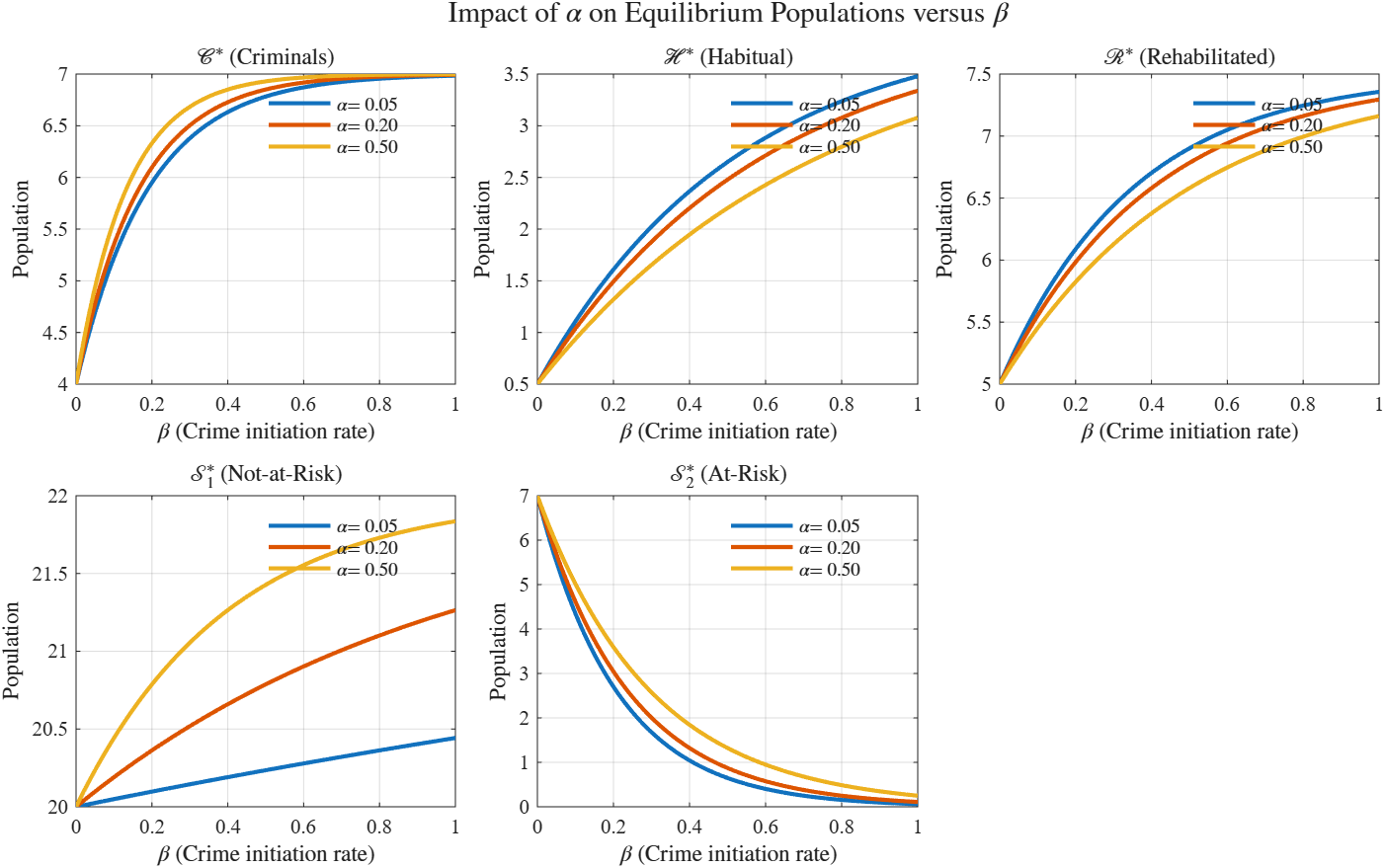
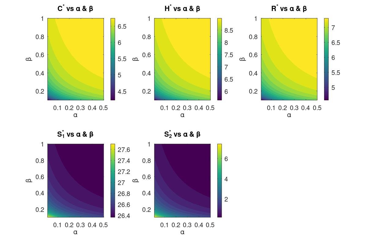
To understand the influence of intervention strategies on crime dynamics, we examined the equilibrium values of five key subpopulations: active criminals (\(C^*\)), habitual criminals (\(H^*\)), rehabilitated individuals (\(R^*\)), not-at-risk individuals (\(S_1^*\)), and at-risk individuals (\(S_2^*\)). These values were analyzed as functions of two critical parameters: \(\alpha\) (the transition rate from susceptibility to crime), varied from \(0.01\) to \(0.5\), and \(\beta\) (the exit or recovery rate from the at-risk group), varied from \(0.1\) to \(1.0\). Initially, we generated line plots showing how these equilibrium populations change with \(\beta\) for three fixed values of \(\alpha = \{0.05, 0.2, 0.5\}\). These plots, presented in Figure 10, demonstrate that an increase in \(\beta\) generally leads to a reduction in the at-risk (\(S_2^*\)) and not-at-risk (\(S_1^*\)) populations, while criminal, habitual, and rehabilitated populations tend to increase, particularly when \(\alpha\) is large. To visualize the combined effect of varying both \(\alpha\) and \(\beta\), we also generated two-dimensional contour plots of the same five populations over a full \((\alpha, \beta)\) grid. Figure 11 illustrates these surfaces, highlighting nonlinear interactions: criminal-related populations (\(C^*\), \(H^*\), \(R^*\)) increase with both \(\alpha\) and \(\beta\), while the susceptible groups (\(S_1^*\) and \(S_2^*\)) exhibit significant decay with increasing \(\alpha\). These plots collectively provide strong evidence that reducing \(\alpha\) (e.g., through prevention programs) and increasing \(\beta\) (e.g., via rehabilitation or education) can mitigate the long-term criminal prevalence in the population.
To analyze the qualitative behavior of the proposed crime dynamics model, we first recall basic notions from the theory of continuous-time dynamical systems [5– 8]. These concepts provide a formal framework for understanding the time evolution, invariance, and equilibrium structure of nonlinear models such as (9).
Definition 2(Dynamical System). A continuous-time dynamical system is defined by the system of ordinary differential equations \[\label{eq:general_system} \frac{d {\mathcal{U}}}{dt} = {\mathcal{F}}( {\mathcal{U}}), \qquad {\mathcal{U}}(0) = {\mathcal{U}}_0 \in \mathbb{R}_+^n, \tag{8}\] where \( {\mathcal{U}} = (\mathcal{U}_1, \ldots, \mathcal{U}_n)^\top\) is the state vector and \( {\mathcal{F}}:\mathbb{R}_+^n \to \mathbb{R}^n\) is a continuously differentiable vector field representing the rate of change of the system variables.
The solution \( {\mathcal{U}}(t)\) traces a trajectory in the phase space \(\mathbb{R}_+^n\). An equilibrium point \( {\mathcal{U}}^*\) satisfies \( {\mathcal{F}}( {\mathcal{U}}^*)= {0}\). The local stability of \( {\mathcal{U}}^*\) is determined by the eigenvalues of the Jacobian matrix \(J = D {\mathcal{F}}( {\mathcal{U}}^*)\) [9].
The nonlinear crime dynamics system (1)–(5) divides the total population into five interacting compartments: not-at-risk \((\mathcal{S}_1)\), at-risk \((\mathcal{S}_2)\), active criminals \((\mathcal{C})\), habitual offenders \((\mathcal{H})\), and rehabilitated or convicted individuals \((\mathcal{R})\). The model can be written compactly in the vector form
\[\label{eq:crime_vector} \frac{d {\mathcal{X}}}{dt} = {\mathcal{F}}( {\mathcal{X}}), \quad \text{where} \quad {\mathcal{X}} = \begin{bmatrix} \mathcal{S}_1 \\[4pt] \mathcal{S}_2 \\[4pt] \mathcal{C} \\[4pt] \mathcal{H} \\[4pt] \mathcal{R} \end{bmatrix}, \qquad {\mathcal{F}}( {\mathcal{X}}) = \begin{bmatrix} (1-p)\pi + (1-q)\gamma \mathcal{R} – (\mu+\theta)\mathcal{S}_1 + \epsilon \mathcal{S}_2 \\[4pt] p\pi – \beta \mathcal{S}_2\mathcal{C}(1+\alpha\mathcal{C}) – (\mu+\epsilon)\mathcal{S}_2 + \theta \mathcal{S}_1 \\[4pt] \beta \mathcal{S}_2\mathcal{C}(1+\alpha\mathcal{C}) + q\gamma \mathcal{R} – (\mu+\sigma+\eta)\mathcal{C} \\[4pt] \eta \mathcal{C} – (\mu+\rho)\mathcal{H} \\[4pt] \sigma \mathcal{C} + \rho \mathcal{H} – (\mu+\gamma)\mathcal{R} \end{bmatrix}. \tag{9}\]
The compact representation (9) enables the use of standard dynamical systems tools—such as equilibrium analysis, nullcline geometry, and the next-generation matrix method—to study the model’s stability and persistence [5].
Lemma 1(Nullclines of the Criminal and At-Risk Compartments).Let \( {\mathcal{X}}(t)\) be the solution of the system (9) within the feasible region \(\Omega\). Then the nullclines corresponding to the criminal and at-risk populations are given by: \[ \mathcal{N}_{\mathcal{C}} = \Big\{( {\mathcal{X}}) \in \Omega : \beta \mathcal{S}_2 \mathcal{C} (1+\alpha \mathcal{C}) + q\gamma \mathcal{R} = (\mu + \sigma + \eta)\mathcal{C} \Big\}, \label{eq:C_nullcline} \ \tag{10}\] \[\mathcal{N}_{\mathcal{S}_2} = \Big\{( {\mathcal{X}}) \in \Omega : p\pi + \theta \mathcal{S}_1 = \big(\mu + \epsilon + \beta \mathcal{C}(1+\alpha \mathcal{C})\big)\mathcal{S}_2 \Big\}. \label{eq:S2_nullcline} \tag{11}\]
Any interior equilibrium \((\mathcal{S}_1^*,\mathcal{S}_2^*,\mathcal{C}^*,\mathcal{H}^*,\mathcal{R}^*)\) satisfies \(\dot{\mathcal{C}}=0\) and \(\dot{\mathcal{S}}_2=0\), i.e., \[(\mathcal{S}_1^*,\mathcal{S}_2^*,\mathcal{C}^*,\mathcal{H}^*,\mathcal{R}^*) \in \mathcal{N}_{\mathcal{C}} \cap \mathcal{N}_{\mathcal{S}_2}.\]
Proof. The nullcline \(\mathcal{N}_{\mathcal{C}}\) is obtained by setting \(\dot{\mathcal{C}}=0\) in (9); similarly, \(\mathcal{N}_{\mathcal{S}_2}\) arises from \(\dot{\mathcal{S}}_2=0\). Since any equilibrium point requires \(\dot{\mathcal{C}}=\dot{\mathcal{S}}_2=0\), the intersection of these nullclines characterizes the interior equilibria. ◻
Lemma 2(Uniform Persistence).Let \(\Omega\) be the feasible region and \(E_0\) the crime-free equilibrium. If the basic reproduction number \(R_c\) satisfies \(R_c>1\), then the system (9) is uniformly persistent: there exists \(\varepsilon>0\) such that for any interior initial condition, \[\liminf_{t\to\infty} \mathcal{C}(t) > \varepsilon, \qquad \liminf_{t\to\infty} \mathcal{H}(t) > \varepsilon,\] and the crime-free equilibrium \(E_0\) is unstable.
Consider the nonlinear system of ordinary differential equations: \[ f_1(S_1, S_2, C, H, R) = (1-p)\pi + (1-q)\gamma R – (\mu + \theta)S_1 + \epsilon S_2, \ \tag{12}\] \[f_2(S_1, S_2, C, H, R) = p\pi – \beta S_2 C (1+\alpha C) – (\mu + \epsilon) S_2 + \theta S_1, \ \tag{13}\] \[f_3(S_1, S_2, C, H, R) = \beta S_2 C (1+\alpha C) + q\gamma R – (\mu + \sigma + \eta) C, \ \tag{14}\] \[f_4(S_1, S_2, C, H, R) = \eta C – (\mu + \rho)H, \ \tag{15}\] \[f_5(S_1, S_2, C, H, R) = \sigma C + \rho H – (\mu + \gamma) R. \tag{16}\]
Define the state vector \[\mathbf{x} = \begin{pmatrix} S_1 \\ S_2 \\ C \\ H \\ R \end{pmatrix}, \quad \frac{d\mathbf{x}}{dt} = \mathbf{f}(\mathbf{x}),\] where \(\mathbf{f}(\mathbf{x}) = (f_1, f_2, f_3, f_4, f_5)^\top\).
The Jacobian matrix of \(\mathbf{f}\), denoted by \(J = D\mathbf{f}(\mathbf{x})\), is the \(5\times5\) matrix of first-order partial derivatives: \[J = \begin{pmatrix} -(\mu+\theta) & \epsilon & 0 & 0 & h_1 \\ \theta & -h_2 & -h_3 & 0 & 0 \\ 0 & h_2 & h_3 – (\mu+\sigma+\eta) & 0 & h_1 \\ 0 & 0 & \eta & -(\mu+\rho) & 0 \\ 0 & 0 & \sigma & \rho & -(\mu+\gamma) \end{pmatrix},\] where \[h_1 = (1-q)\gamma, \qquad h_2 = \beta C(1+\alpha C), \qquad h_3 = \beta S_2(1+2\alpha C).\]
The local stability of an equilibrium point \(\mathbf{x}^* = (S_1^*, S_2^*, C^*, H^*, R^*)\) is determined by the eigenvalues of \(J^* = J(\mathbf{x}^*)\). The characteristic polynomial associated with \(J^*\) is: \[\lambda^5 + a_4 \lambda^4 + a_3 \lambda^3 + a_2 \lambda^2 + a_1 \lambda + a_0 = 0,\] where the coefficients \(a_i\) are functions of the model parameters and equilibrium values.
The expressions for \(a_0, a_1, a_2, a_3\), and \(a_4\) are derived symbolically (see supplementary appendix for full derivations). For completeness, the first two coefficients are given by: \[a_0 = 1, \qquad a_1 = \eta + \gamma + h_2 – h_3 + 4\mu + \rho + \sigma + \theta.\]
Higher-order coefficients (\(a_2, a_3, a_4, a_5\)) involve nonlinear combinations of \(\mu\), \(\sigma\), \(\rho\), \(\gamma\), \(\eta\), and \(h_i\) terms and are omitted here for brevity.
By the Abel–Ruffini theorem, there exists no general closed-form solution in radicals for a fifth-degree (or higher) polynomial: \[P(\lambda) = a_5 \lambda^5 + a_4 \lambda^4 + a_3 \lambda^3 + a_2 \lambda^2 + a_1 \lambda + a_0, \quad a_5 \neq 0.\]
Hence, the eigenvalues of \(J^*\) must be computed numerically. This theorem establishes that symbolic expressions for the eigenvalues of high-dimensional nonlinear systems, such as the present crime dynamics model, are not generally obtainable.
Lemma 3. Let \((S_1^*, S_2^*, C^*, H^*, R^*)\) denote an equilibrium point of system (1)–(5), and let \(J^*\) be the Jacobian matrix evaluated at this equilibrium. Then, the equilibrium is locally asymptotically stable if and only if all eigenvalues \(\lambda_i\) of \(J^*\) satisfy \(\operatorname{Re}(\lambda_i) < 0\) for \(i=1,\dots,5\). If at least one eigenvalue satisfies \(\operatorname{Re}(\lambda_i) > 0\), the equilibrium is unstable.
This criterion follows directly from the Hartman–Grobman theorem and standard linearization principles for nonlinear dynamical systems [8, 10].
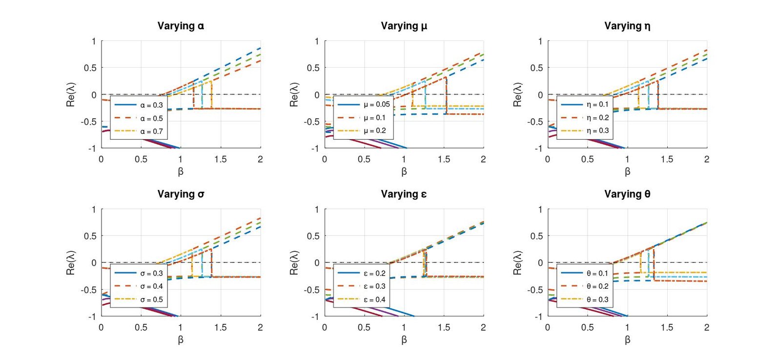
Figure 12 illustrates the dependence of system stability on six key parameters—\(\alpha\), \(\mu\), \(\eta\), \(\sigma\), \(\epsilon\), and \(\theta\). Each subplot displays the real parts of the dominant eigenvalues \((\lambda_3, \lambda_4, \lambda_5)\) as functions of the crime initiation rate \(\beta\). The dashed horizontal line \(\operatorname{Re}(\lambda)=0\) marks the stability threshold separating stable and unstable regimes. The observations are summarized as follows:
Effect of \(\alpha\) (susceptible-to-criminal transition): Increasing \(\alpha\) from 0.3 to 0.7 shifts instability onset to lower \(\beta\) values, indicating that stronger peer influence or imitation accelerates the transition toward crime-dominated dynamics.
Effect of \(\mu\) (natural removal or exit rate): Raising \(\mu\) (e.g., from 0.05 to 0.2) stabilizes the system by reducing eigenvalue magnitudes, signifying that natural attrition or rehabilitation efforts mitigate long-term instability.
Effect of \(\eta\) (habitual criminality): Higher \(\eta\) values amplify instability by pushing eigenvalues toward positive real parts. Persistent offenders thus represent a destabilizing factor in social equilibrium.
Effect of \(\sigma\) (conviction rate): Increasing \(\sigma\) from 0.3 to 0.5 enhances stability by keeping eigenvalues negative over larger \(\beta\) intervals, emphasizing the effectiveness of strong law enforcement.
Effect of \(\epsilon\) (awareness and prevention): Larger \(\epsilon\) values expand the stable region, suggesting that preventive programs and public awareness initiatives delay the onset of instability.
Effect of \(\theta\) (rate of becoming habitual): As \(\theta\) rises from 0.1 to 0.3, eigenvalues cross into the positive region earlier, indicating that faster progression toward habitual behavior increases the risk of instability.
Overall, all parameter sweeps exhibit bifurcation-like transitions as \(\operatorname{Re}(\lambda)\) crosses zero. The position of this transition delineates the stability boundary and highlights the critical influence of \(\alpha\), \(\eta\), and \(\mu\) on the persistence or decay of crime within the modeled population.
The disease-free equilibrium occurs when \(C = 0\) (no criminal activity). Substituting \(C = 0\), \(H = 0\), and \(R = 0\) into the system reduces it to:
\[ (1-p)\pi – (\mu+\theta)S_1 + \epsilon S_2 = 0 \ \tag{17}\] \[p\pi – (\mu+\epsilon)S_2 + \theta S_1 = 0 \ \tag{18}\] \[S_1 + S_2 = \frac{\pi}{\mu}. \tag{19}\]
Solving this linear system yields the disease-free equilibrium: \[E_0 = \left( S_1^0, S_2^0, 0, 0, 0 \right),\] where \[S_1^0 = \frac{\pi[\mu(1-p) + \epsilon]}{\mu(\mu + \theta + \epsilon)}, \quad S_2^0 = \frac{\pi(p\mu + \theta)}{\mu(\mu + \theta + \epsilon)}.\]
This equilibrium represents a crime-free society where:
\(S_1^0\): Non-risk individuals (rehabilitated or never at risk)
\(S_2^0\): At-risk individuals (potential criminals but not active)
All other compartments (\(C, H, R\)) are empty
The DFE is biologically feasible (\(S_1^0, S_2^0 > 0\)) for all \(\pi, \mu, \theta, \epsilon > 0\) and \(0 \leq p \leq 1\).
The Jacobian matrix \(J\) is \[J = \begin{pmatrix} -(\mu + \theta) & \epsilon \\ \theta & -(\mu + \epsilon) \end{pmatrix}.\]
The characteristic equation for eigenvalues \(\lambda\) is given by \[\det(J – \lambda I) = 0,\] i.e., \[\det \begin{pmatrix} -(\mu + \theta) – \lambda & \epsilon \\ \theta & -(\mu + \epsilon) – \lambda \end{pmatrix} = 0,\] which expands to \[\left(-(\mu + \theta) – \lambda\right) \left(-(\mu + \epsilon) – \lambda\right) – \epsilon \theta = 0.\]
Simplifying, this gives the quadratic equation: \[\lambda^2 + \lambda (2\mu + \epsilon + \theta) + \mu^2 + \mu(\epsilon + \theta) = 0.\]
The eigenvalues \(\lambda\) can then be found by the quadratic formula: \[\lambda = \frac{-(2\mu + \epsilon + \theta) \pm \sqrt{(2\mu + \epsilon + \theta)^2 – 4(\mu^2 + \mu(\epsilon + \theta))}}{2}.\]
The basic reproduction number \(\mathcal{R}_0\) represents the expected number of new criminals generated by a single criminal in a fully susceptible population. We compute it using the next-generation matrix method.
Define the infected compartments as \(\mathbf{I} = [C, H, R]^T\). The linearized system at \(E_0\) is:
\[\frac{d\mathbf{I}}{dt} = (\mathbf{F} – \mathbf{V})\mathbf{I},\] where \(\mathbf{F}\) (new infections) and \(\mathbf{V}\) (transitions) are: \[\mathbf{F} = \begin{bmatrix} \beta S_2^0 & 0 & 0 \\ 0 & 0 & 0 \\ 0 & 0 & 0 \end{bmatrix}, \quad \mathbf{V} = \begin{bmatrix} \mu+\sigma+\eta & 0 & -q\gamma \\ -\eta & \mu+\rho & 0 \\ -\sigma & -\rho & \mu+\gamma \end{bmatrix}.\]
The next-generation matrix is \(\mathbf{K} = \mathbf{F}\mathbf{V}^{-1}\). The spectral radius \(\rho(\mathbf{K})\) gives \(\mathcal{R}_0\). Since \(\mathbf{F}\) has only one non-zero entry:
\[\mathcal{R}_0 = \beta S_2^0 \cdot [\mathbf{V}^{-1}]_{11},\] where \([\mathbf{V}^{-1}]_{11}\) is the (1,1)-entry of \(\mathbf{V}^{-1}\). The determinant of \(\mathbf{V}\) is: \[\det(\mathbf{V}) = (\mu+\sigma+\eta)(\mu+\rho)(\mu+\gamma) – q\gamma[\eta\rho + \sigma(\mu+\rho)].\]
The (1,1)-entry of \(\mathbf{V}^{-1}\) is: \[[\mathbf{V}^{-1}]_{11} = \frac{(\mu+\rho)(\mu+\gamma)}{\det(\mathbf{V})}.\]
Substituting \(S_2^0\) and simplifying yields:
\[\boxed{\mathcal{R}_0 = \frac{\beta \pi (p\mu + \theta) (\mu + \rho)(\mu + \gamma)}{\mu (\mu + \theta + \epsilon) \left[ (\mu + \sigma + \eta)(\mu + \rho)(\mu + \gamma) – q\gamma (\eta \rho + \sigma (\mu + \rho)) \right]}}\]
Interpretation of \(\mathcal{R}_0\):
Threshold Value: \(\mathcal{R}_0 = 1\) determines the stability of \(E_0\)
Epidemiological Meaning:
\(\mathcal{R}_0 < 1\): Each criminal produces fewer than one new criminal \(\implies\) crime dies out
\(\mathcal{R}_0 > 1\): Each criminal produces more than one new criminal \(\implies\) crime persists
Key Parameters:
\(\beta\): Crime transmission rate (\(\uparrow \beta \implies \uparrow \mathcal{R}_0\))
\(q\): Recidivism rate (\(\uparrow q \implies \uparrow \mathcal{R}_0\))
\(\gamma\): Rehabilitation rate (\(\uparrow \gamma \implies \downarrow \mathcal{R}_0\))
\(\sigma\): Conviction rate (\(\uparrow \sigma \implies \downarrow \mathcal{R}_0\))
Significance:
A transcritical bifurcation occurs at \(\mathcal{R}_0 = 1\), where \(E_0\) loses stability and an endemic equilibrium emerges
To achieve crime eradication (\(\mathcal{R}_0 < 1\)), interventions should:
Decrease \(\beta\) through prevention programs
Increase \(\gamma\) through rehabilitation
Increase \(\sigma\) through law enforcement
Decrease \(q\) through reintegration programs
The nonlinear term \(\alpha C\) implies crime self-reinforcement, making eradication more challenging once established
To investigate the sensitivity of the reproduction number \(\mathcal{R}_c\) to variations in model parameters, a series of contour plots were generated for different parameter pairs, as shown in Figure 13. In each subplot, the red dashed line marks the critical threshold \(\mathcal{R}_c = 1\), which separates the regions of persistence (\(\mathcal{R}_c > 1\)) and elimination (\(\mathcal{R}_c < 1\)) of criminal activity.
The contour plots illustrate how combinations of key parameters influence the potential for crime proliferation:
Plot (a): Increasing either the crime transmission rate \(\beta\) or the fraction of newly recruited individuals entering the at-risk class \(p\) raises \(\mathcal{R}_c\). A broader region above the \(\mathcal{R}_c = 1\) threshold implies greater risk of sustained crime.
Plot (b): As the natural removal rate \(\mu\) increases, \(\mathcal{R}_c\) decreases, indicating that higher exit or mortality rates diminish the potential for crime propagation.
Plot (c): Increasing the conviction rate \(\sigma\) reduces \(\mathcal{R}_c\), emphasizing the stabilizing effect of efficient law enforcement mechanisms.
Plot (d): A higher habitual progression rate \(\eta\) elevates \(\mathcal{R}_c\), particularly when \(p\) is large, revealing that persistent offenders drive system instability.
Plot (e): The combination of low \(\mu\) and high \(\beta\) generates conditions most favorable to crime persistence, suggesting that stable or slow-changing populations face greater criminal sustainability risks.
Plot (f): Joint increases in \(\mu\) and \(\sigma\) markedly lower \(\mathcal{R}_c\), showing that natural turnover combined with effective policing produces a synergistic suppressive effect on crime.
These results suggest that policy interventions should prioritize reducing \(p\), \(\beta\), and \(\eta\), while enhancing \(\mu\), \(\sigma\), or \(\epsilon\) to maintain \(\mathcal{R}_c < 1\) and achieve long-term crime control.
To complement the contour analysis, three-dimensional surface plots were produced to visualize the combined influence of key parameter pairs on \(\mathcal{R}_c\), as shown in Figure 14. These surfaces provide a more continuous and intuitive understanding of how parameter interactions shape the reproduction dynamics of criminal activity.
Plot (a): \(\mathcal{R}_c\) increases smoothly with both \(p\) and \(\beta\), confirming that stronger recruitment into the at-risk class and higher transmission rates jointly amplify crime persistence.
Plot (b): As \(\mu\) increases, \(\mathcal{R}_c\) declines, illustrating how natural exit mechanisms weaken criminal networks.
Plot (c): Increasing conviction rate \(\sigma\) leads to a sharp drop in \(\mathcal{R}_c\), particularly for large \(p\), emphasizing the deterrent effect of robust law enforcement.
Plot (d): Larger values of \(\eta\) increase \(\mathcal{R}_c\), unless mitigated by smaller \(p\), underscoring the need to disrupt habitual criminal progression.
Plot (e): A strong nonlinear interaction is observed—high \(\beta\) combined with low \(\mu\) causes rapid escalation of \(\mathcal{R}_c\), identifying this as a critical risk region.
Plot (f): Joint increases in \(\mu\) and \(\sigma\) produce steep declines in \(\mathcal{R}_c\), revealing synergistic effects between natural turnover and judicial deterrence.
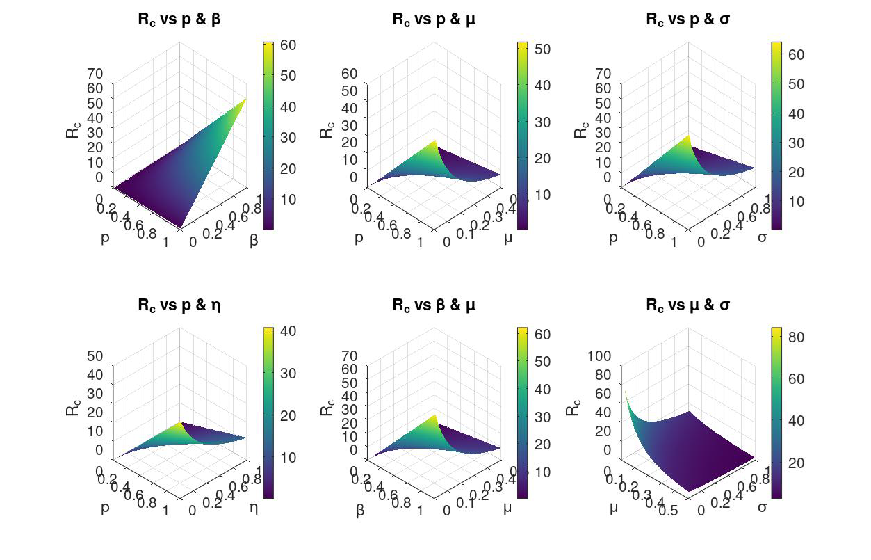
Overall, the contour and surface visualizations consistently demonstrate that maintaining \(\mathcal{R}_c < 1\) requires simultaneous management of multiple socio-behavioral and law-enforcement parameters. These findings offer quantitative guidance for policy optimization in crime prevention and control strategies.
In this study, we developed and analyzed a nonlinear compartmental model of crime dynamics that partitions the population into five interacting groups: not-at-risk, at-risk, active criminals, habitual criminals, and rehabilitated individuals. Through analytical and numerical investigation, we explored how variations in the crime initiation rate (\(\alpha\)) and the reintegration rate of at-risk individuals (\(\beta\)) influence the overall crime dynamics. The simulations revealed that higher \(\alpha\) values substantially increase both the criminal and habitual populations, whereas lower \(\beta\) values hinder the successful rehabilitation of at-risk individuals. Line and contour plots demonstrated that reducing susceptibility to criminal influence (i.e., decreasing \(\alpha\)) and enhancing reformation efforts (i.e., increasing \(\beta\)) are crucial for minimizing persistent criminal activity. We further derived the basic reproduction number \(\mathcal{R}_c\), which serves as a threshold indicator for the persistence or eradication of criminal behavior. Sensitivity analysis indicated that \(\mathcal{R}_c\) is particularly responsive to key parameters such as the crime transmission rate (\(\beta\)), recruitment into the at-risk group (\(p\)), natural exit rate (\(\mu\)), conviction rate (\(\sigma\)), and progression to habitual crime (\(\eta\)). Contour and 3D surface plots identified critical parameter regions where \(\mathcal{R}_c < 1\) corresponds to crime suppression, while \(\mathcal{R}_c > 1\) signifies sustained or growing criminal activity. These findings emphasize that reducing recruitment and transmission rates, enhancing conviction and rehabilitation efforts, and increasing natural exit mechanisms can collectively drive \(\mathcal{R}_c\) below unity—thereby mitigating long-term crime prevalence. The local stability analysis further confirmed that increases in crime-promoting parameters such as \(\alpha\) and \(\eta\) destabilize the equilibrium, whereas higher values of \(\mu\), \(\sigma\), and the public awareness rate (\(\epsilon\)) enhance stability. Eigenvalue bifurcation patterns with respect to \(\beta\) revealed critical transition points, highlighting the model’s sensitivity to small parameter perturbations and potential for bifurcation-induced behavioral shifts. Overall, this work provides a comprehensive mathematical framework for understanding crime propagation and control. By integrating equilibrium analysis, reproduction threshold estimation, and stability investigation, the study offers quantitative insights to guide evidence-based crime prevention and rehabilitation policies, contributing to the long-term goal of achieving sustainable social stability.