
Privacy has always been an issue from both sociological and legal point of views. The first definition of privacy was made by Warren and Brandeis as the right to be let alone and further research showed that the limits of the privacy concept are hard to set as they are context-dependent, rely on the individual autonomy and the intentions for information processing [1,2]. Thus, the personal data plays a key role in assessing privacy. According to Directive 95/46/EC, personal data is any information relating to an identified or identifiable natural person, and later legislative acts including General Data Protection Regulation pointed out the necessity to assess the sensitivity of the data considering identifiability and the purpose of the data processing [3–5].
Nowadays, there is a need for privacy-aware analysis with the increase of the number of data-intensive systems. The methods like differential privacy and privacy-aware machine learning guarantee protection of the individual during the process of data processing, however, the process of risk assessment needs to be preceded by identification of the variables that might be sensitive or even potentially sensitive [6–8]. In many databases, this step cannot be done easily as some variables are obviously private as they contain the information about the finance, demographics, health and the way of living of the user and others seem to be non-sensitive on their own but become sensitive when highly correlated with the private variables.
The research problem is if the feature selection techniques can be used to predict the privacy status of potentially private variables based on the known private ones. The novelty of this research is the interpretation of existing filter-based feature selection techniques in terms of the privacy-risk analysis. Namely, feature ranking will be transformed into the pairwise distance between features and then the variables carrying implicit privacy information will be detected based on those distances.
Personal data occur in internet usage, healthcare, shopping, financials, legal matters, and public administration. Privacy aspects vary depending on the area, but there are four groups in particular that deserve attention.
It is clear from the above examples why privacy assessment cannot rely solely on variable names. Even if a certain attribute is not considered private explicitly, it can disclose personal information due to being statistically or semantically similar to a private attribute.
Risk management is a process of identifying the risks, evaluating their importance, prioritizing and making decisions whether the risk should be mitigated, accepted, transferred or monitored [9]. Common risk management standards include the terminology and methodology for risk evaluation: ISO 31000 and ISO/IEC Guide 73 [10,11]. Privacy risk management differs from the traditional security risk management by including both the external threats and internal factors like sensitivity of the information, identification and usage context [12,13].
A scoring process is the most common way to represent the results of risk assessment. The simple scores can be obtained through average, summation or categorization while more complex score evaluation uses statistical or data mining models like regression, LOGIT, PROBIT, classification [14]. The information security risk literature distinguishes between qualitative evaluations producing labels like low, medium and high risk and quantitative evaluations resulting in numbers [15,16]. An example of the use of domain-specific rules in privacy evaluation can be found in privacy impact assessment and HIPAA legislation [17,18]. Recently published privacy guidance calls for the identification of privacy relevant data elements prior to the choice of risk controls [19].
Privacy-related risk assessment involves determining of the asset value depending on whether the information can identify, describe and expose a person. Known private variables can be defined through the regulations and domain knowledge but the identification of potentially private variables needs relational analysis. For instance, age, education level, native country and so on are not always considered as private but their relation to occupation, income, ethnicity or marital status significantly increases privacy risk.
The proposed method determines the privacy status of uncertain variables using their relevance to variables with known privacy status. Consider the feature space
which consists of variables \(F\) of the data set and the set of observations \(V\). For any variable \(f_j\) in the set, the rest of the variables are considered candidate predictors,
Feature selection and weighting methods assign weights to elements in \(X_j\) to assess their relevancy to \(f_j\). We then transform the ranking into pairwise distance and interpret the variables with distance below some predefined threshold as relevant pairs. The problem is predictive in the sense that we infer the privacy status of uncertain variables based on their relationship with private variables at the feature level.
The rest of the paper is organized as follows. Feature selection and feature weighting are introduced in §2. The relevance-distance method is described in §3. The experiment is presented in §4. Implications and conclusions are discussed
Feature selection is a technique that decreases the number of variables used in a data mining task through the identification of relevant variables for the target concept [20]. The feature selection algorithms can be supervised, unsupervised, or semi-supervised depending on whether target labels are available [21]. The results generated by these algorithms are typically in the form of a list of variables ranked by their relevance, or a selected subset.
The two popular approaches are filter models and wrapper models [22]. Filter models rely on various data characteristics such as association, correlation, entropy, statistical dependence to assess the quality of variables. The filter models are generally computationally inexpensive and classifier-independent. In contrast, wrapper models evaluate subsets of variables using a learning algorithm which means that they directly optimize classifier performance but they are more expensive than filter models.
Relevance and redundancy are the key concepts of feature selection. Relevance is an assessment of the strength of relationship between a feature and the target variable. Redundancy is the similarity in the information provided by two or more features. If \(Q(F^i)\) is the score of the candidate feature subset \(F^i\subseteq F\), then univariate scoring function evaluates individual features while multivariate scoring function evaluates a subset. While univariate scoring function is more computationally efficient, multivariate scoring function can capture interaction between features [21,23]. The search strategies include individual ranking, forward search, and backward search [24]. Individual ranking searches one feature at a time, forward search starts with an empty subset and adds new useful features while backward search starts from the whole set and removes unnecessary features.
The advantage of feature selection approach to privacy-risk analysis is that it reveals the connections that might not be apparent from the labels of the features. The potentially private feature in isolation does not imply anything, its relevance is defined by the information it provides on the private feature. Thus, filter approach is most suitable for this task due to interpretability of its output.
The relevance measures are computed using the filter model algorithms since they do not depend on the specific classifier and assess the relevance at data level. Each feature is used sequentially as a target and all others are predictors. As a result, the list of directed relevance measures is constructed and aggregated into the distance matrix.
The algorithm is presented in Fig. 1. Three filtering techniques are applied for each feature \(f_j\) as a target and a set of predictor features \(X_j\) is taken as an input. These filtering techniques are chi-square filtering, correlation-based feature selection (CFS) and fast correlation-based filtering (FCBF). Relevant features identified by these filters form a distance vector \(d_j\). The same procedure is repeated for all \(f_j \in F\) resulting in a feature-distance matrix.
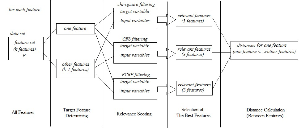
Then the distance matrix is transformed to the set of relevant pairs. By \(d_{ji}\) we denote the distance from a target feature \(f_j\) to a predictor feature \(f_i\). The pairs are selected when the value of distance does not exceed the threshold \(\tau\):
Threshold \(\tau=5\) is used in the experiments. If the known private feature is connected to a feature from the set \(\mathcal{P}_{\tau}\), such a feature is considered as potentially private. The inference procedure is demonstrated in Fig. 2. The rule is intentionally conservative and selects variables that need further attention regarding the issue of privacy.
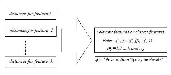
The main component of the method is the scoring of relevance. The chosen filtering methods are appropriate as they give various perspectives of relevance: marginal association, subset correlation and relevance-redundancy balance.
The chi-square test measures whether the distribution of a predictor is statistically independent of the target variable [25]. For categorical variables, the chi-square statistic is
where \(O_{rc}\) and \(E_{rc}\) are the observed and expected frequencies in cell \((r,c)\). Larger values indicate stronger dependence between the predictor and the target. In feature selection, predictors can therefore be ranked according to their chi-square scores.
Correlation-based feature selection evaluates a feature subset by favoring variables that are highly correlated with the target but weakly correlated with each other [26]. For a subset with \(s\) features, the CFS merit can be expressed as
where \(\bar r_{cf}\) is the mean feature-class correlation and \(\bar r_{ff}\) is the mean feature-feature correlation. This criterion is useful for privacy analysis because it selects variables that explain the target while reducing redundant evidence.
FCBF is designed for high-dimensional data and combines relevance analysis with redundancy removal [27]. It commonly uses symmetric uncertainty,
where \(IG(X\mid Y)\) is information gain and \(H(\cdot)\) is entropy. Features with high relevance to the target are retained, while redundant features are removed according to their symmetric uncertainty values. In this paper, FCBF complements chi-square and CFS by emphasizing non-linear information-theoretic association.
The experimental analysis uses the Adult data set from the UCI Machine Learning Repository [28]. The data were extracted from the 1994 United States census database and contain 48,842 records. The table contains demographic, work-related, financial, and income-class variables. These variables are suitable for privacy analysis because several of them are directly linked to financial position, family status, ethnicity, occupation, and demographic identity.
| Feature name | Type | Sample values |
|---|---|---|
| age | continuous | 10, 14, 27, 34, 50, \(\ldots\) |
| workclass | categorical | Self-emp-not-inc, Self-emp-inc, Federal-gov, \(\ldots\) |
| fnlwgt | continuous | 77516, 83311, 338409, \(\ldots\) |
| education | categorical | Bachelors, Some-college, 11th, HS-grad, Prof-school, \(\ldots\) |
| education-num | continuous | 13, 9, 8, 11, \(\ldots\) |
| marital-status | categorical | Married-civ-spouse, Divorced, Never-married, \(\ldots\) |
| occupation | categorical | Tech-support, Craft-repair, Other-service, Sales, \(\ldots\) |
| relationship | categorical | Wife, Own-child, Husband, Not-in-family, \(\ldots\) |
| race | categorical | White, Asian-Pac-Islander, Amer-Indian-Eskimo, \(\ldots\) |
| sex | categorical | Female, Male |
| capital-gain | continuous | 1200, 2450, 300, 678, \(\ldots\) |
| capital-loss | continuous | 0, 100, 230, 900, \(\ldots\) |
| hours-per-week | continuous | 40, 13, 36, \(\ldots\) |
| native-country | categorical | United-States, Cambodia, England, Puerto-Rico, \(\ldots\) |
| class | categorical | \(\leq 50\)K, \(>50\)K |
In the original table, there are fifteen columns when considering the income class as a variable. Three variables, namely fnlwgt, education-num, and hours-per-week, were not included in the relevance analysis due to being derived, poorly aligned with the privacy question, or not being among the chosen privacy interpretations. The other twelve variables were named as follows: workclass (\(F_1\)), education (\(F_2\)), marital-status (\(F_3\)), occupation (\(F_4\)), relationship (\(F_5\)), race (\(F_6\)), sex (\(F_7\)), native-country (\(F_8\)), income class (\(F_9\)), age (\(F_{10}\)), capital-gain (\(F_{11}\)), and capital-loss (\(F_{12}\)).
The experiment aims to find the potentially private variables through the measurement of relations between each target feature and other features. The experiment consists of three steps. In the first step, twelve features are prepared for the filtering procedure. Specifically, all continuous variables which are used in the experiment, namely age, capital-gain, and capital-loss, are transformed into categorical values since the chosen filtering procedures work only with categorical data. In the second step, every feature is taken as the target one while the remaining eleven features are considered as predictors. Then, in the third step, chi-square filtering, CFS filtering, and FCBF filtering are performed for each target-predictor pair.
For every target feature, the relevant or ranked features provided by the three filtering procedures are combined. In case when the number of relevant features exceeds three for some filter, only top-three ranked features are selected for comparability of the output lists of the three filters. Next, the ranking outputs are translated into distances. The greater the rank of some feature, the greater its distance value; in case when the feature is not included in the list of relevant features, the maximum possible distance contribution is assigned. The obtained distance values lie between 0 and 9 where 0 means the maximum observed relevance and 9 corresponds to the absence of the selected relevance. The pairs with distance values at most \(\tau=5\) are considered non-trivial.
| Target variable | Filter model | ||
|---|---|---|---|
| Chi-square filtering | CFS filtering | FCBF filtering | |
| Workclass (\(F_1\)) | 0 – Occupation 1 – Class 2 – Sex | 0 – Occupation | 0 – Occupation 1 – Race |
| Education (\(F_2\)) | 0 – Class 1 – Occupation 2 – Native-country | 0 – Occupation 1 – Native-country 2 – Class | 0 – Occupation 1 – Native-country 2 – Class |
| Marital-status (\(F_3\)) | 0 – Relationship 1 – Sex 2 – Class | 0 – Relationship | 0 – Relationship 1 – Class 2 – Age |
| Occupation (\(F_4\)) | 0 – Workclass 1 – Sex 2 – Education | 0 – Workclass 1 – Education 2 – Sex | 0 – Workclass 1 – Education 2 – Sex |
| Relationship (\(F_5\)) | 0 – Marital-status 1 – Sex 2 – Class | 0 – Marital-status | 0 – Marital-status 1 – Race 2 – Sex |
| Race (\(F_6\)) | 0 – Native-country 1 – Relationship 2 – Sex | 0 – Native-country | 0 – Relationship 1 – Native-country |
| Sex (\(F_7\)) | 0 – Relationship 1 – Marital-status 2 – Occupation | 0 – Relationship | 0 – Occupation 1 – Relationship |
| Native-country (\(F_8\)) | 0 – Race 1 – Education 2 – Occupation | 0 – Race | 0 – Race 1 – Education |
| Class (\(F_9\)) | 0 – Relationship 1 – Marital-status 2 – Sex | 0 – Marital-status 1 – Relationship 2 – Education | 0 – Marital-status 1 – Education 2 – Capital-gain |
| Age (\(F_{10}\)) | 0 – Marital-status 1 – Relationship 2 – Class | 0 – Marital-status 1 – Relationship 2 – Education | 0 – Education 1 – Marital-status 2 – Hours-per-week |
| Capital-gain (\(F_{11}\)) | 0 – Class 1 – Age 2 – Relationship | 0 – Class | 0 – Native-country 1 – Class 2 – Age |
| Capital-loss (\(F_{12}\)) | 0 – Class 1 – Age 2 – Relationship | 0 – Marital-status 1 – Class | 0 – Native-country 1 – Class |
Table 2 gives the individual ranking results from the three filters. The following relations are found to be consistent from the results, namely workclass – occupation, marital status – relationship, race – native country and income class – relationship, marital status, education and capital gain. The above results are realistic since the Adult data set involves socio-economic variables with distributional dependencies.
Table 3 presents the distance matrix based on the output in Table 2. Small distances mean stronger relations. For instance, the distance value between workclass and occupation is 0 since occupation is chosen as the relation with workclass in the filter results. On the other hand, the distance value of 9 means the relation is not present. The cut-off value of \(\tau=5\) is used for distinguishing strong relations.
| \(F_1\) | \(F_2\) | \(F_3\) | \(F_4\) | \(F_5\) | \(F_6\) | \(F_7\) | \(F_8\) | \(F_9\) | \(F_{10}\) | \(F_{11}\) | \(F_{12}\) | |
|---|---|---|---|---|---|---|---|---|---|---|---|---|
| \(F_1\) | – | 9 | 9 | 0 | 9 | 7 | 8 | 9 | 7 | 9 | 9 | 9 |
| \(F_2\) | 9 | – | 9 | 1 | 9 | 9 | 9 | 4 | 4 | 9 | 9 | 9 |
| \(F_3\) | 9 | 9 | – | 9 | 0 | 9 | 7 | 9 | 6 | 8 | 9 | 9 |
| \(F_4\) | 0 | 4 | 9 | – | 9 | 9 | 5 | 9 | 9 | 9 | 9 | 9 |
| \(F_5\) | 9 | 9 | 0 | 9 | – | 7 | 6 | 9 | 8 | 9 | 9 | 9 |
| \(F_6\) | 9 | 9 | 9 | 9 | 4 | – | 8 | 1 | 9 | 9 | 9 | 9 |
| \(F_7\) | 9 | 9 | 7 | 5 | 1 | 9 | – | 9 | 9 | 9 | 9 | 9 |
| \(F_8\) | 9 | 5 | 9 | 8 | 9 | 0 | 9 | – | 9 | 9 | 9 | 9 |
| \(F_9\) | 9 | 6 | 1 | 9 | 4 | 9 | 8 | 9 | – | 9 | 8 | 9 |
| \(F_{10}\) | 9 | 5 | 1 | 9 | 5 | 9 | 9 | 9 | 8 | – | 9 | 9 |
| \(F_{11}\) | 9 | 9 | 9 | 9 | 8 | 9 | 9 | 6 | 1 | 6 | – | 9 |
| \(F_{12}\) | 9 | 9 | 6 | 9 | 8 | 9 | 9 | 6 | 2 | 7 | 9 | – |
At \(\tau=5\), the relevant pair set is
These pairs are reorganized by target variable in Table 4. This presentation makes the privacy interpretation clearer because it shows which predictors are closest to each target feature.
| Target variable | Relevant predictor variables |
|---|---|
| \(F_1\) | \(F_4\) |
| \(F_2\) | \(F_4\), \(F_8\), \(F_9\), \(F_{10}\) |
| \(F_3\) | \(F_5\), \(F_9\), \(F_{10}\) |
| \(F_4\) | \(F_1\), \(F_2\), \(F_7\) |
| \(F_5\) | \(F_3\), \(F_6\), \(F_7\), \(F_9\) |
| \(F_6\) | \(F_5\) |
| \(F_7\) | \(F_4\), \(F_5\) |
| \(F_8\) | \(F_2\), \(F_6\) |
| \(F_9\) | \(F_2\), \(F_3\), \(F_5\), \(F_{11}\), \(F_{12}\) |
| \(F_{10}\) | \(F_3\), \(F_5\) |
| \(F_{11}\) | \(F_9\) |
| \(F_{12}\) | \(F_9\) |
This matrix provides two kinds of evidence. First, it determines compact relevance neighborhoods. With income class (\(F_9\)) as the target, relevant features are education (\(F_2\)), marital-status (\(F_3\)), relationship (\(F_5\)), capital-gain (\(F_{11}\)), and capital-loss (\(F_{12}\)). To check if these dependencies have predictive value, two tests with C4.5 classifiers were performed [29]. With all predictors used in a model, the 10-fold cross-validation achieved 85% accuracy, and with the relevant predictors of \(F_9\) only – 83%. The slight accuracy difference shows that the relevant-feature subset carries almost all necessary information for predicting income class. Thus, this fact confirms the validity of the distance-based relevance output.
Second, this matrix can be used for inferring the privacy-status of features. The set of known private seed features includes workclass (\(F_1\)), marital-status (\(F_3\)), occupation (\(F_4\)), and race (\(F_6\)). Features workclass and occupation correspond to financial and employment privacy, respectively; marital-status corresponds to lifestyle privacy; and race to ethnicity-related privacy. By using the threshold rule and interpreting domains, we conclude that the potentially private variables are relationship (\(F_5\)), sex (\(F_7\)), native-country (\(F_8\)), income class (\(F_9\)), and age (\(F_{10}\)). Although features education (\(F_2\)), capital-gain (\(F_{11}\)), and capital-loss (\(F_{12}\)) exhibit relevance, they need explicit policy interpretation, since their privacy status depends on data use and the extent of regulation.
This classification is therefore more useful than just a per variable classification. As mentioned above, there are four private variables in the known set, and relevance analysis adds five potentially private variables to be considered. For privacy risk analysis, this result means that the process of privacy scoring should take into account not only the variables which are explicitly designated as private, but also those which are located nearby in the feature-distance structure.
The empirical results provide affirmative answer to the research question: feature selection algorithms can contribute to predicting potentially private data items when the results of the latter are translated into interpretable relevance distances. Variables like relationship, sex, native-country, income-level, and age in the Adult data set are privacy-relevant because they are proximate to private variables in the distance matrix. This finding is particularly valuable because the traditional practice of privacy risk assessment starts with a list of fixed private fields while in reality there are indirect dependencies that may reveal private information despite of the non-sensitive field name.
The empirical findings provide evidence of the scientific benefit of using several filter methods. Chi-square filtering reveals a high marginal dependence, CFS achieves balance between feature-target association and redundancy control, FCBF adds information-theoretical criterion for relevance-redundancy evaluation. Thus, combining the output of all three algorithms helps to reduce dependence on one criteria and formulates the distance matrix for inspection by the privacy analyst. At the same time, C4.5 test for the income-level provides proof that the identified relevant variables contain most of the predictive content of the entire predictor set. Thus, it is clear that the detected relations contain information about sensitive targets and not just descriptive power.
From privacy perspective, the result means that the risk scoring should be based not only on the field name but also on the relationship among fields. In the conducted experiment, the set of directly known private variables has been expanded into a set of privacy-relevant variables. It leads to a more sensitive estimation of personal-data risk since the method allows detecting implicit privacy channels. However, at the same time the proposed method does not substitute legal and domain judgment of private fields. The low distance value does not mean the legal sensitivity. The variables like education, capital-gain, and capital-loss represent the example: they are close to the income or employment variable in the sense of relevance, but the final status of these variables from the point of view of privacy should be determined based on the purpose of processing and other factors.
The main drawback of the work is the demonstration of the technique on one public data set with discrete continuous variables and a fixed relevance threshold. The threshold regulates the level of strictness of pairs selection and different data sets require different threshold values. The second drawback is the conservative approach to privacy inference: the emphasis is made on direct relationships to the known private variables and no free propagation through the chain of association is allowed. These drawbacks are not essential but they require validation on additional data sets prior to operational use of the method.
In conclusion, the study shows that popular feature selection algorithms can be applied to detect indirect privacy relationships among data attributes. By translating the output of filter algorithm into a feature-distance matrix, the method detects potential privacy variables because of their proximity to the known private variables. For the Adult data set, the method finds four variables known to be private and marks five additional variables which are worth privacy attention.
Acknowledgments: The author appreciates the support of Cumhuriyet University, Computer Engineering Department.
Conflicts of Interest: The author declares no conflict of interest.