
Nonlinear vibrating systems are fundamental to many engineering and scientific endeavours. The time-domain response of the undamped motion of these systems is characterized by symmetric or asymmetric vibrations. The systems exhibiting symmetric vibration possess odd-parity stiffness nonlinearity about the relevant equilibrium, whereas asymmetric vibrations may arise when the restoring force also contains even-parity terms about the chosen reference point. However, some systems possess both odd-parity and even-parity nonlinearities and are said to have mixed-parity nonlinearity. The latter systems are generic and can exhibit either symmetric or asymmetric vibrations depending on the restoring force and the oscillation interval.
A key area of interest in the study of nonlinear vibrations is the solution of the nonlinear ordinary differential equation (NODE) modeling the vibration response. A useful technique to develop approximate analytical solutions to the NODE is to apply the exact solution of a simpler equivalent system. In this regard, the most common approach is the equivalent linearization method (ELM) that uses the exact solution of an equivalent linear ODE to find the approximate solution of ODEs with non-polynomial nonlinearities, i.e., \(\ddot u+\omega_{eq}^{2}u=0\) where \(\omega_{eq}\) is the frequency of the equivalent linear system that approximates the nonlinear frequency. Several authors have combined the principle of equivalent linearization with other techniques to develop approximate analytical solutions for nonlinear vibration models. Belendez et al. [1] applied the ELM with asymptotic Taylor’s series expansion of the exact time integral to determine the optimal parameter for estimation of \(\omega_{eq}\). Belendez et al. [2] used the asymptotic Chebyserv series expansion to improve the optimal parameter for estimation of \(\omega_{eq}\) based on the ELM. He [3] applied the ELM to derive a simple amplitude-frequency solution for conservative oscillators with odd nonlinearities. The approximate nonlinear frequency was derived by evaluating the first derivative of the nonlinear restoring force at a location point. The main drawback of the simple amplitude-frequency solution is that the location point that minimizes the error of the estimated nonlinear frequency is based on a guess. El-Dib [4] extended the simple amplitude-frequency solution based on ELM to obtain the approximate periodic solution and the damped nonlinear frequency of non-conservative oscillators. Hieu [5] applied an ELM based on weighted averaging to develop an approximate solution to a generalized nonlinear oscillator. The results of the method showed an improved accuracy compared to other ELMs such as the energy balance method [6], the amplitude-frequency formula [7], and the variational approach [8]. Moatimid et al. [9] proposed a non-perturbative method for the solution of highly nonlinear oscillators using an ELM with weighted residuals to estimate the nonlinear frequency. The non-perturbative method was based on an earlier ELM by El-Dib [10] that was developed to find approximate periodic solutions for mixed-parity nonlinear oscillators.
The ELMs can provide a good estimate for the nonlinear frequency of vibrating systems even under conditions of strong nonlinear response. However, a single-harmonic ELM cannot reproduce an anharmonic profile during strong nonlinear vibration, e.g., the near-buckling vibration response of a functionally-graded microbeam [11]. This is because that form of ELM uses a simple harmonic solution for the vibration history. As a result, other equivalent oscillators have been proposed, such as the cubication methods [12–17] in which oscillators with non-polynomial nonlinearities are transformed into an equivalent cubic Duffing oscillator, and the quintication methods [18–20] where oscillators with non-polynomial nonlinearities are transformed into an equivalent cubic-quintic Duffing oscillator. Furthermore, Big-Alabo et al. [21] derived an approximate solution to the vibration of the Porter governor using an equivalent non-natural oscillator model. The cubication and quintication formulations discussed above primarily address odd-parity restoring forces. An exception among the equivalent linearization approaches is the ELM by El-Dib [10] that was developed for mixed-parity oscillators. The method was based on treating the odd-parity nonlinearities as secular terms for the derivation of the nonlinear frequency, while the even-parity nonlinearities were treated as non-secular terms that translated into the non-homogeneous part of the equivalent linear oscillator. Its stated zero-initial-velocity formulation does not directly provide the general-initial-state construction considered here. This motivates an amplitude-dependent mixed-parity equivalent oscillator, rather than a claim that methods for asymmetric oscillators are absent.
In this study, an equivalent oscillator model that is based on the mixed-parity Helmholtz-Duffing oscillator (HDO) has been developed for approximate periodic solutions of asymmetric oscillators with non-polynomial nonlinearities. A quasi-static equilibrium approach that has been used in previous studies [17,19,21] was applied to obtain the constants of the equivalent HDO, and then, the exact solution of the HDO was used to obtain an approximate solution for the original nonlinear asymmetric oscillator. The HDO model used for this study is undamped with a constant excitation and generalized initial conditions. Its exact solution was derived from the exact time integral of its vibration model. The specific contribution is the simultaneous matching of the restoring force at zero and at the two unequal turning points, together with the potential-energy difference between them, while retaining the quadratic term and constant load. This is an extension of established equivalent-oscillator constructions; the general initial-state phase prescription extends the use of the known HDO quadrature and is not a separate new integrability result.
The exact periodic solution of the undamped HDO with constant load has been derived in other studies. The common approach is to use an ansatz solution in which the exact solution is forced to take the form of an assumed solution [22–25]. Some such expressions apply only to specified parameter regimes [23]. As an alternative, Big-Alabo and Alfred [26] derived the exact periodic solution of the undamped HDO with constant load from the exact time integral of the HDO model. However, the initial conditions used in their study are non-zero initial displacements and zero initial velocity. Here, the generalized initial conditions with non-zero displacement and velocity are considered. Hence, the exact solution for the undamped HDO with constant load and generalized initial conditions was derived here from the exact time integral. This exact solution was then applied to obtain the approximate analytical solution for asymmetric oscillators with non-polynomial nonlinearities.
Consider the undamped HDO with arbitrary stiffness constants, a constant force, and generalized initial conditions as shown in Eq. (1):
\[\tag{1} \frac{d^2w}{dt^2}+k_1w+k_2w^2+k_3w^3+F=0,\] where the initial conditions are: \(w(0)=w_0\) and \(\dot w(0)=v_0\), and \((w_0,v_0)\in\mathbb R^2\) can take both zero and non-zero values. The coefficients in Eq. (1) are normalized by the relevant mass or inertia. The following quartic formulas require \(k_3\ne0\) and a non-equilibrium bounded orbit with distinct turning points \(w_2<w_1\). These are the adjacent real roots enclosing the initial state on its connected admissible energy interval, where the radicand in Eq. (2) is positive. Equilibria, separatrices and escaping trajectories are not finite-period cases covered by these formulas; general initial conditions do not imply that every real initial state is periodic. Integrating Eq. (1) and applying the generalized initial conditions gives the first integral: \[\tag{2} \frac{dw}{dt}=\pm\sqrt{v_0^2+2F(w_0-w)+k_1(w_0^2-w^2)+\frac{2}{3}k_2(w_0^3-w^3)+\frac{1}{2}k_3(w_0^4-w^4)},\] from which we get the exact time integral as: \[\tag{3} \int dt=\pm\int\frac{dw}{\sqrt{v_0^2+2F(w_0-w)+k_1(w_0^2-w^2)+\frac{2}{3}k_2(w_0^3-w^3)+\frac{1}{2}k_3(w_0^4-w^4)}}.\]
The goal is to demonstrate that Eq. (3) is in fact an elliptic integral that can be solved in terms of the standard Legendre forms through various algebraic transformations, closed-form solutions of the roots of a general quartic equation, and the use of standard tables of elliptic integrals.
To evaluate the time period, the integration of Eq. (3) must be done over a half-cycle because the HDO is an asymmetric oscillator. Then, the time period can be expressed as: \[\tag{4} T_{ex}=2\int_{w_2}^{w_1}\frac{dw}{\sqrt{v_0^2+2F(w_0-w)+k_1(w_0^2-w^2)+\frac{2}{3}k_2(w_0^3-w^3)+\frac{1}{2}k_3(w_0^4-w^4)}},\] where \(w_1\) and \(w_2\) are the maximum displacements or amplitudes and generally \(|w_1|\ne|w_2|\). Although the amplitudes can be unequal, the potential energies at both amplitudes are equal i.e. \(V(w_1)=V(w_2)\), where \(V(w)=h(w,0)\) with \(h\) defined in Appendix B. The condition \(k_2=0\) alone does not imply equal-magnitude amplitudes when \(F\ne0\). Eq. (4) can be written as: \[\tag{5} T_{ex}=2\sqrt{\frac{2}{k_3}}\int_{w_2}^{w_1}\frac{dw}{\sqrt{a_0+a_1w+a_2w^2+a_3w^3-w^4}},\] where \[\tag{6} a_3=-\frac{4k_2}{3k_3};\quad a_2=-\frac{2k_1}{k_3};\quad a_1=-\frac{4F}{k_3};\quad a_0=w_0^4+\frac{2}{k_3}\left(v_0^2+2Fw_0+k_1w_0^2+\frac{2k_2}{3}w_0^3\right).\]
At the amplitudes, the HDO attains its maximum potential energy along the selected orbit, whereas the kinetic energy is zero. The implication is that the amplitudes, \(w_1\) and \(w_2\), are solutions to the quartic equation \[\tag{7} a_0+a_1w+a_2w^2+a_3w^3-w^4=0.\]
The possibility of solving Eq. (5) in closed-form depends on deriving algebraic solutions for the quartic equation in Eq. (7). Although algebraic solutions for a general quartic equation are well established [27–29], they are usually presented in a complicated manner with many different conditions that are not organized systematically. Therefore, to derive a straightforward solution for Eq. (7), we have applied a simplified systematic form of Ferrari’s solution for a general quartic equation (See Appendix A).
A quartic equation need not have real roots; here the assumed bounded orbit supplies the two real turning points. The remaining two roots can be a complex-conjugate pair or two additional real roots. With the turning points selected from the initial energy interval, the quartic expression in Eq. (5) can be factored as follows:
\[\tag{8} T_{ex}=2\sqrt{\frac{2}{k_3}}\int_{w_2}^{w_1}\frac{dw}{\sqrt{(w_1-w)(w-w_2)(w-w_3)(w-w_4)}},\] where \(w_1\) and \(w_2\) are the selected real roots, and \(w_3\) and \(w_4\) are the remaining roots.
The real roots (\(w_1\) and \(w_2\)) can be obtained from the depressed form of the quartic equation using Ferrari’s method (see appendix A). On the other hand, the remaining two roots were obtained from the quadratic equation derived after dividing Eq. (7) by the product of the two selected real factors, i.e. \[\tag{9} w^2+(\lambda_1+w_2)w+(\lambda_2+\lambda_1w_2+w_2^2)=0,\] where \[\tag{10} \lambda_1=w_1-a_3,\qquad \lambda_2=w_1(w_1-a_3)-a_2.\]
Therefore, \[\tag{11} w_3,w_4=\frac{-(\lambda_1+w_2)\pm i\sqrt{4(\lambda_2+\lambda_1w_2+w_2^2)-(\lambda_1+w_2)^2}}{2},\] where \(i=\sqrt{-1}\). Eq. (11) also represents two real roots when its inner radicand is negative, with consistent complex square-root evaluation.
Having obtained closed-form solutions to the roots of the quartic equation, we now proceed to determine the period in terms of elliptic integrals. For this purpose, we can use the list of standard elliptic integrals provided by Byrd and Friedman [30]. In particular, we are interested first in the integral of a quartic expression where two of the factors are complex conjugates. Formula 259.00 on page 133 of Byrd and Friedman [30] provides the following result: \[\tag{12} \int_b^y\frac{dz}{\sqrt{(a-z)(z-b)(z-c)(z-\bar c)}}=G\times F(\varphi,m),\] where \(F(\varphi,m)\) is the incomplete elliptic integral of the first kind defined as: \[\tag{13} F(\varphi,m)=\int_0^\varphi(1-m\sin^2\theta)^{-1/2}\,d\theta,\] and the arguments of \(F(\varphi,m)\) are defined as: \[\tag{14a} \varphi=\cos^{-1}\!\left[\frac{(a-y)Q-(y-b)P}{(a-y)Q+(y-b)P}\right],\] \[\tag{14b} m=\frac{(a-b)^2-(P-Q)^2}{4PQ}.\]
Also, \[\tag{14c} G=\frac{1}{\sqrt{PQ}};\quad P=\sqrt{(a-r_2)^2+r_1^2};\quad Q=\sqrt{(b-r_2)^2+r_1^2};\quad r_2=\frac{c+\bar c}{2};\quad r_1=\sqrt{-\frac{(c-\bar c)^2}{4}},\]
Applying Eqs. (12 – 14a) in Eq. (8), the exact time period was derived as: \[\tag{15} T_{ex}=\frac{4K(m)}{\psi}\] where, \(K(m)\) is the complete elliptic integral of the first kind. For \(0<m\le0.999\), the algebraic formula in Big-Alabo [31] provides an approximation; an assertion of machine-epsilon accuracy additionally requires a stated precision and error check. Also, \[\tag{16a} m=\frac12-\frac{3w_2^2+3w_1w_2+\lambda_1(w_1+3w_2)+2\lambda_2}{4\sqrt{w_1^2+w_2^2+w_1(\lambda_1+w_2)+\lambda_1w_2+\lambda_2}\sqrt{3w_2^2+2\lambda_1w_2+\lambda_2}},\] \[\tag{16b} \psi=\left[\frac{k_3}{2}\sqrt{w_1^2+w_2^2+w_1(\lambda_1+w_2)+\lambda_1w_2+\lambda_2}\sqrt{3w_2^2+2\lambda_1w_2+\lambda_2}\right]^{1/2}.\]
The product \(PQ\) is evaluated using the two separate square roots, \[PQ=\sqrt{w_1^2+w_2^2+w_1(\lambda_1+w_2)+\lambda_1w_2+\lambda_2}\sqrt{3w_2^2+2\lambda_1w_2+\lambda_2},\] rather than replacing them by a principal square root of their product. For a bounded orbit with \(k_3<0\), \(P\) and \(Q\) have the same imaginary phase, so that \(PQ<0\) while \(k_3PQ>0\). For four real roots, the conjugate-pair premise of Eq. (12) no longer applies directly. The same substitution in Eq. (22) remains applicable with \(P^2=(w_1-w_3)(w_1-w_4)\) and \(Q^2=(w_2-w_3)(w_2-w_4)\): choose a common real or imaginary phase for \(P,Q\), take \(\psi>0\), and require a real \(m<1\) and a nonzero displacement denominator. These conditions make the displacement real and recover the first integral. Negative values of \(m\) are permitted and require direct evaluation of \(K(m)\) rather than the positive-parameter approximation just cited. Square roots in Eqs. (5) and (8) must likewise be evaluated on consistent branches.
Taking the limits of the left-hand side of Eq. (3) from \(0\) to \(t\) implies that the corresponding limits of the right-hand side will be from \(w_0\) to \(w\). For \(v_0\ne0\), on the initial monotone segment, retain the direction factor \(\sigma_0\) defined in Eq. (26). Hence, we have: \[\tag{17} \sigma_0t=\int_{w_0}^{w}\frac{dw}{\sqrt{v_0^2+2F(w_0-w)+k_1(w_0^2-w^2)+\frac{2}{3}k_2(w_0^3-w^3)+\frac12k_3(w_0^4-w^4)}}.\]
Using the results of the earlier algebraic transformation, Eq. (17) can be written as: \[\begin{aligned} \sigma_0t={}&\sqrt{\frac{2}{k_3}}\int_{w_0}^{w}\frac{dw}{\sqrt{(w_1-w)(w-w_2)(w-w_3)(w-w_4)}}\notag\\ ={}&\sqrt{\frac{2}{k_3}}\left[\int_{w_2}^{w}\frac{dw}{\sqrt{(w_1-w)(w-w_2)(w-w_3)(w-w_4)}}-\int_{w_2}^{w_0}\frac{dw}{\sqrt{(w_1-w)(w-w_2)(w-w_3)(w-w_4)}}\right]. \end{aligned}\tag{18}\]
The direction factor accounts for whether the initial velocity is negative or positive. The integral identities hold on the initial monotone segment; the elliptic displacement formula provides the continuation through subsequent turning points.
Using Eqs. (12 – 14a) and Eq. (18), we get: \[\tag{19} \sigma_0t+t_0=\frac{1}{\psi}F(\varphi,m),\] where \(\psi\) is given in Eq. (16b), \(F(\varphi,m)\) is defined in Eq. (13), and \(t_0\) is the nonnegative phase time between the lower turning point \(w_2\) and the initial displacement \(w_0\) and is given as: \[\tag{20} t_0=\frac{1}{\psi}F(\varphi_0,m).\]
The constant \(\varphi_0\) is computed as: \[\tag{21} \varphi_0=\cos^{-1}\!\left[\frac{(w_1-w_0)Q-(w_0-w_2)P}{(w_1-w_0)Q+(w_0-w_2)P}\right],\] where \(P=\sqrt{w_1^2+w_2^2+w_1(\lambda_1+w_2)+\lambda_1w_2+\lambda_2}\) and \(Q=\sqrt{3w_2^2+2\lambda_1w_2+\lambda_2}\). Also, from Eqs. (14a) and (18) we have: \[\tag{22} \cos\varphi=\frac{(w_1-w)Q-(w-w_2)P}{(w_1-w)Q+(w-w_2)P}.\]
The elliptic amplitude (\(\varphi\)) is the inverse of the incomplete elliptic integral of the first kind, and can be obtained from Eq. (19) as: \(\varphi=F^{-1}(\psi(\sigma_0t+t_0),m)\). Applying the definition and evenness of the Jacobi cosine function, i.e. \(\cos\varphi=\cos[F^{-1}(\psi(\sigma_0t+t_0),m)]=\operatorname{cn}[\psi(t+\sigma_0t_0),m]\) and using Eq. (22), we get: \[\tag{23} \operatorname{cn}[\psi(t\pm t_0),m]=\frac{(w_1-w)Q-(w-w_2)P}{(w_1-w)Q+(w-w_2)P}.\]
Solving for \(w\) in Eq. (23) gives the exact displacement response of the HDO as: \[\tag{24} w(t)=\frac{w_2P+w_1Q+(w_2P-w_1Q)\operatorname{cn}[\psi(t\pm t_0),m]}{P+Q+(P-Q)\operatorname{cn}[\psi(t\pm t_0),m]}.\]
In Eq. (24), the plus sign applies if \(v_0>0\) and the minus sign applies if \(v_0<0\). For \(v_0=0\), the plus sign retains the turning-point phase: \(t_0=0\) at \(w_2\) and \(t_0=T_{ex}/2\) at \(w_1\). Thus, the exact displacement response can be written as: \[\tag{25} w(t)=\frac{w_2P+w_1Q+(w_2P-w_1Q)\operatorname{cn}[\psi(t+\sigma_0t_0),m]}{P+Q+(P-Q)\operatorname{cn}[\psi(t+\sigma_0t_0),m]},\] where \(\sigma_0\) is the phase-direction selector defined as: \[\tag{26} \sigma_0=\begin{cases}-1&\text{if }v_0<0,\\+1&\text{if }v_0=0,\\+1&\text{if }v_0>0.\end{cases}\]
The present exact solution in Eq. (25) can be used for admissible zero initial conditions, non-zero initial conditions, and when only one of the initial conditions is zero. An initial state at equilibrium instead gives the constant solution. The choice \(\sigma_0=1\) when \(v_0=0\) is a phase convention, not an assertion of positive physical velocity at an upper turning point.
In §2, the exact time period and displacement response of an undamped HDO with constant load and generalized initial conditions were derived. In this section, the quasi-static equilibrium principle was used to derive an equivalent HDO for asymmetric oscillators with non-polynomial nonlinearities. It is a common practice to derive equivalent nonlinear oscillators using Taylor’s series expansion of the original nonlinear restoring force. However, a fixed low-order Taylor’s series approximation can be inaccurate for large-amplitude vibrations outside the neighbourhood of its expansion point [14]. To address this shortcoming and improve the accuracy of equivalent nonlinear oscillators, some studies have applied the Chebyserv series expansion to derive stiffness constants that account for the amplitude [14,15,18,20]. Although the Chebyserv series expansion can converge rapidly for sufficiently regular restoring forces, deriving the stiffness constant for oscillators with non-polynomial nonlinearities is algebraically complicated and may involve the application of special functions [19]. An alternative approach for deriving stiffness constants that account for the amplitude is the quasi-static equilibrium approach [16,19,31]. Hence, the quasi-static equilibrium approach was applied here to derive the equivalent HDO.
The quasi-static equilibrium approach is based on the idea that the restoring force of a nonlinear conservative oscillator undergoing rate-independent motion can be estimated by a simpler polynomial function (i.e., an equivalent restoring force) using quasi-static considerations. To this end, the quasi-static responses of the original nonlinear oscillator and the equivalent oscillator can be matched to determine the stiffness constants of the equivalent oscillator.
Let us consider a general conservative asymmetric oscillator of the form \[\tag{27} \frac{d^2w}{dt^2}+g(w)=0,\] where \(g(-w)\ne-g(w)\); \(g(w)\) is an asymmetric restoring force with non-polynomial nonlinearities, and the initial conditions are \(w(0)=w_0\) and \(\dot w(0)=v_0\). The force is assumed to be real and continuous on the selected oscillation interval, with a well-defined potential and finite \(g(0)\); differentiability is additionally needed wherever stiffness matching is invoked. The initial energy must determine a bounded connected interval with two distinct turning points.
An approximate solution to Eq. (27) can be obtained from the solution of an equivalent HDO as shown: \[\tag{28} \frac{d^2w}{dt^2}+f(w)=0,\] where \(f(w)=k_1w+k_2w^2+k_3w^3+F\) and the initial conditions are the same as Eq. (27). The stiffness constants (\(k_1\), \(k_2\) and \(k_3\)) and the constant load (\(F\)) of the equivalent oscillator are unknown and can be derived based on selected force, energy, and stiffness quasi-static equilibrium conditions.
Force equilibrium condition: requires that the restoring force of the original nonlinear asymmetric oscillator and the equivalent HDO should be equal at zero displacement and at the amplitudes. \[\tag{29a}f(0)=g(0),\] \[\tag{29b}f(A)=g(A),\] \[\tag{29c}f(B)=g(B),\] where \(A\) and \(B\) are the amplitude and biased amplitude, respectively, which were determined from the roots of the nonlinear algebraic equation describing the energy balance of the original nonlinear asymmetric oscillator, as shown: \[\tag{30} V(w_{max})=\frac12v_0^2+V(w_0),\] where \(V(w)=\int g(w)\,dw\) is the potential function and \(w_{max}\) is the maximum displacement representing the amplitudes \(A\) and \(B\). Only the adjacent roots bounding the connected admissible interval containing \(w_0\) are used; other potential wells and escaping branches are excluded. The labels \(A\) and \(B\) need not denote positive and negative values.
Energy equilibrium condition: requires that the potential-energy difference over a half-cycle is the same for the original nonlinear asymmetric oscillator and the equivalent HDO. \[\tag{31} \int_B^A f(w)\,dw=\int_B^A g(w)\,dw.\]
The potential function of a conservative nonlinear asymmetric oscillator gives the same value at the amplitudes \(A\) and \(B\). This implies that both sides of Eq. (31) will evaluate to zero. Nevertheless, Eq. (31) provides one of the mathematical equations that can be used to determine the stiffness constants of the equivalent HDO.
Stiffness equilibrium condition: requires that the stiffness (i.e., first derivative of the restoring force) of the original nonlinear asymmetric oscillator and the equivalent HDO should be equal at the amplitudes. \[\tag{32a}f'(A)=g'(A),\] \[\tag{32b}f'(B)=g'(B).\]
The force and stiffness equilibrium conditions give rise to single-point displacement matching, while the energy equilibrium condition provides for matching over a range of the displacement. The resulting Eqs. (29a – 32a) provide six candidate conditions from which the four unknown constants of the equivalent HDO can be derived. Only Eqs. (29a) and (31) are imposed here; the stiffness conditions in Eqs. (32a) and (32b) are not additional properties of the resulting approximation. These four conditions give: \[\tag{33}F=g(0),\] \[\tag{34}k_1A+k_2A^2+k_3A^3+F=g(A),\] \[\tag{35}k_1B+k_2B^2+k_3B^3+F=g(B),\] \[\tag{36}6k_1(A^2-B^2)+4k_2(A^3-B^3)+3k_3(A^4-B^4)+12F(A-B)=0.\]
Eq. (33) gives the constant load of the equivalent HDO. On the other hand, the stiffness constants were derived by solving Eqs. (34) to (36) simultaneously. Hence, \[\tag{37} k_1=-\frac{g(0)\mu_0+B^2g(A)\mu_1+A^2g(B)\mu_2}{A(A-B)^3B(A+B)},\] \[\tag{38} k_2=\frac{3[g(0)\lambda_0+g(A)\lambda_1+g(B)\lambda_2]}{A(A-B)^3B},\] \[\tag{39} k_3=-\frac{2[g(0)\lambda_0+g(A)\lambda_3+g(B)\lambda_4]}{A(A-B)^3B(A+B)},\] where \[\tag{40a–h} \left.\begin{aligned} \mu_0&=(A-B)^3(A^2+4AB+B^2),\\ \mu_1&=(B-A)(3A^2+2AB+B^2),\\ \mu_2&=(B-A)(A^2+2AB+3B^2),\\ \lambda_0&=(A-B)^3,\\ \lambda_1&=B(B^2-A^2),\\ \lambda_2&=A(B^2-A^2),\\ \lambda_3&=B(B-A)(2A+B),\\ \lambda_4&=A(B-A)(A+2B). \end{aligned}\right\}\]
The results in Eqs. (37 – 40a–h) show that the stiffness constants of the equivalent HDO depend on the amplitudes \(A\) and \(B\), and the value of the original nonlinear restoring force at zero displacement and at the amplitudes. The \(\lambda\) symbols in Eq. (40a–h) are local matching constants and are distinct from the root-division constants in Eq. (10).
Eqs. (37)–(39) require \(AB(A-B)(A+B)\ne0\). Zero or symmetric fitting amplitudes and the limit of coalescing turning points cannot be handled by direct substitution into these fractions; the underlying linear system must be examined separately. No uniform conditioning or accuracy guarantee is claimed near these singular limits. To apply the construction, first determine \(A,B\) from Eq. (30), evaluate \(g(0),g(A),g(B)\), and calculate the coefficients from Eqs. (33) and (37)–(40a–h). Then use the same \(w_0,v_0\) in the equivalent HDO, recompute its turning points from Eq. (7), and verify the bounded-orbit and branch conditions of §2 before evaluating its period and displacement. The half-cycle condition makes the equivalent potential equal at \(A\) and \(B\), but does not generally match its potential difference from an interior \(w_0\). Consequently, for nonzero initial velocity, \(A,B\) are fitting points and need not be the actual turning points of the equivalent HDO. This distinction is essential for comparisons under identical initial conditions. Solving the original amplitude equation can require numerical root finding; the construction is not an entirely closed-form procedure for an arbitrary non-polynomial force.
The exact time period and displacement solutions derived in §2 were compared with numerical solutions reported as obtained using the NDSolve and NIntegrate functions in Mathematica. The latter were respectively used for numerical solution of the differential equation and numerical quadrature. In selecting the cases, consideration was given to the conditions for bounded periodic solutions of the HDO prescribed by Geng [23]. In defining these conditions, Geng [23] applied the discriminants and constants given in Appendix B.
Table 1 shows the reported exact time period compared with the corresponding time period of the numerical solutions for various initial and parametric conditions. Thirteen different cases of initial and parametric conditions were examined; these are representative cases, not a proof of coverage of all bounded periodic states. Cases 1, 2, 3 and 5 do not reproduce from Eq. (1) with the listed coefficients and initial conditions. The table entries are retained as reported rather than replaced by unrecorded NDSolve or NIntegrate runs, and these cases cannot validate the corrected formulas. The source computations do not specify working precision, solver tolerances, integration settings, or period-extraction procedures. Agreement between displayed columns alone therefore does not establish numerical accuracy. The energy-sign descriptions in cases 4, 6 and 10 are corrected using Eqs. (B7)–(B12): \(h_{02}<0\) in case 4, \(h_{02}>0\) in case 6, and \(h>0\) in case 10.
| Equation parameter | Numerical | Exact | ||||||
|---|---|---|---|---|---|---|---|---|
| Case | ICs | \(k_1\) | \(k_2\) | \(k_3\) | \(F\) | NDSolve | NIntegrate | Present |
| 1 | \(k_3>0,F\neq0,\Delta_3<0\) | |||||||
| \(\begin{gathered}w_0=1\\v_0=1\end{gathered}\) | 1 | 2 | 3 | 0.1 | 3.41946 | 3.41946 | 3.41946 | |
| 2 | \(k_3>0,F=0,\Delta_4<0\) | |||||||
| \(\begin{gathered}w_0=2\\v_0=5\end{gathered}\) | 15 | 12 | 10 | 0.0 | 0.783199 | 0.783199 | 0.783199 | |
| 3 | \(k_3>0,F\neq0,\Delta_3>0\) | |||||||
| \(\begin{gathered}w_0=0.1\\v_0=2\end{gathered}\) | -4 | 3 | 2 | 0.2 | 3.94796 | 3.94796 | 3.94796 | |
| 4 | \(k_3>0,F=0,k_1>0,k_2>0,\Delta_4>0,h_{02}<0\) | |||||||
| \(\begin{gathered}w_0=3\\v_0=4\end{gathered}\) | 1 | 8 | 5 | 0.0 | 0.960996 | 0.960997 | 0.960996 | |
| 5 | \(k_3<0,F\neq0,\Delta_3>0,h_1>h_3\) | |||||||
| \(\begin{gathered}w_0=0.3\\v_0=1\end{gathered}\) | 20 | 15 | -1 | 0.5 | 1.42968 | 1.42968 | 1.42968 | |
| 6 | \(k_3<0,F=0,k_1<0,k_2>0,\Delta_4>0,h_{02}>0\) | |||||||
| \(\begin{gathered}w_0=1\\v_0=0.6\end{gathered}\) | -5 | 5 | -1 | 0 | 3.73469 | 3.73469 | 3.73469 | |
| 7 | \(k_3>0,F\neq0,\Delta_3>0,h_1>h_3\) | |||||||
| \(\begin{gathered}w_0=0.3\\v_0=1\end{gathered}\) | -5 | -3 | 2 | 4 | 6.43744 | 6.43744 | 6.43744 | |
| 8 | \(k_3>0,F=0,k_1<0,k_2>0,\Delta_4>0\) | |||||||
| \(\begin{gathered}w_0=0.5\\v_0=-5\end{gathered}\) | -7 | 5 | 6 | 0 | 1.92904 | 1.92904 | 1.92904 | |
| 9 | \(k_3>0,F=0,k_1>0,k_2>0,\Delta_4>0,h_{02}<0\) | |||||||
| \(\begin{gathered}w_0=0.5\\v_0=-5\end{gathered}\) | 4 | 5 | 0.5 | 0 | 3.21825 | 3.21824 | 3.21824 | |
| 10 | \(k_3>0,F=0,k_1<0,k_2=0,h\in(0,\infty)\) | |||||||
| \(\begin{gathered}w_0=-0.5\\v_0=3\end{gathered}\) | -1 | 0 | 2 | 0 | 3.14893 | 3.14893 | 3.14893 | |
| 11 | \(k_3>0,F=0,k_1<0,k_2=0,h\in(0,\infty)\) | |||||||
| \(\begin{gathered}w_0=1\\v_0=-3\end{gathered}\) | -10 | 0 | 4 | 0 | 4.19710 | 4.19710 | 4.19710 | |
| 12 | \(k_3>0,F=0,k_1>0,k_2<0,\Delta_4>0,h_{01}<0\) | |||||||
| \(\begin{gathered}w_0=1\\v_0=0.5\end{gathered}\) | 15 | -20 | 0.5 | 0 | 1.94984 | 1.94984 | 1.94984 | |
| 13 | \(k_3<0,F=0,k_1>0,k_2=0\) | |||||||
| \(\begin{gathered}w_0=1\\v_0=3\end{gathered}\) | 25 | 0 | -1 | 0 | 1.28350 | 1.28350 | 1.28350 | |
Reported values retained. Cases 1, 2, 3 and 5 remain inconsistent with the listed initial-value problems; see §4.1.
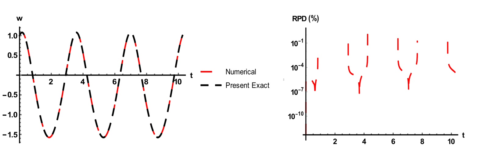
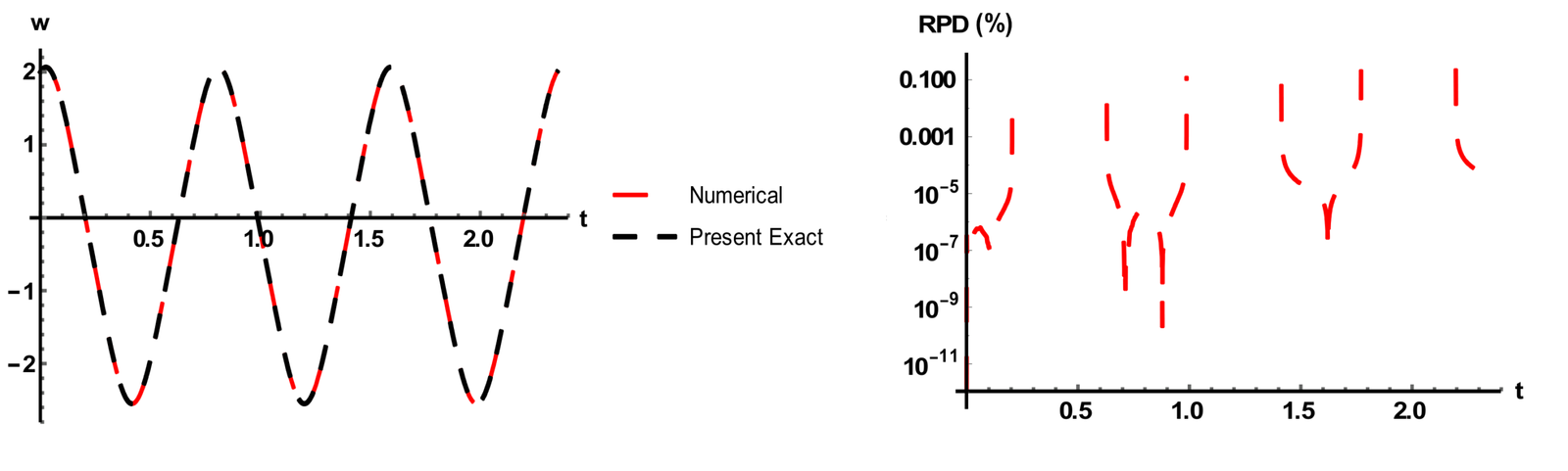
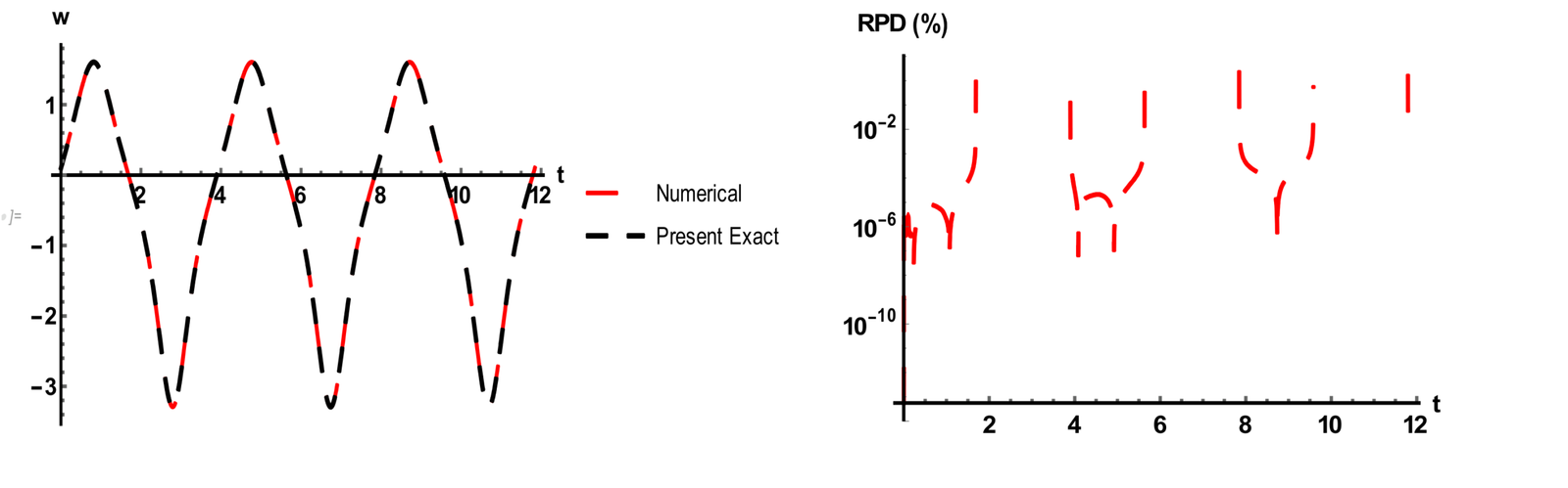
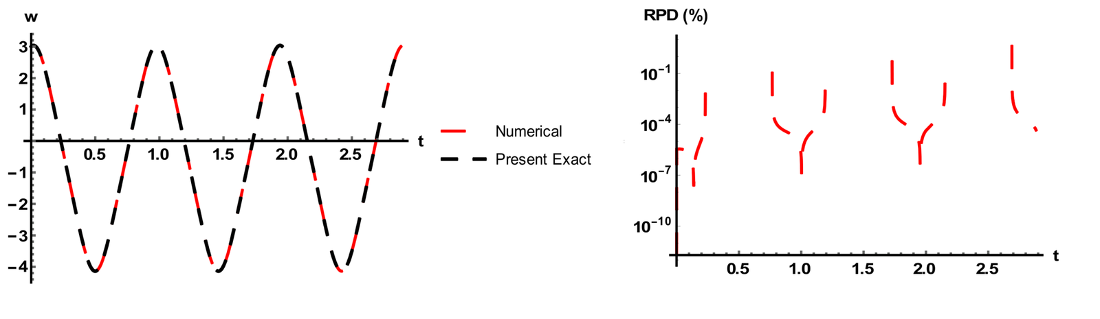
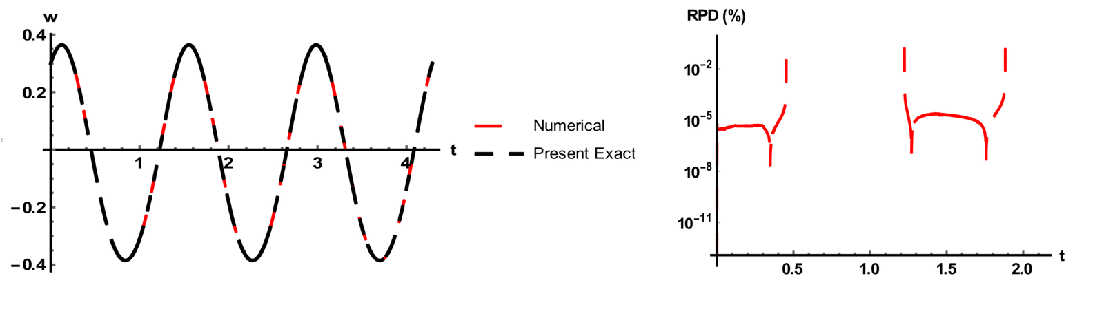
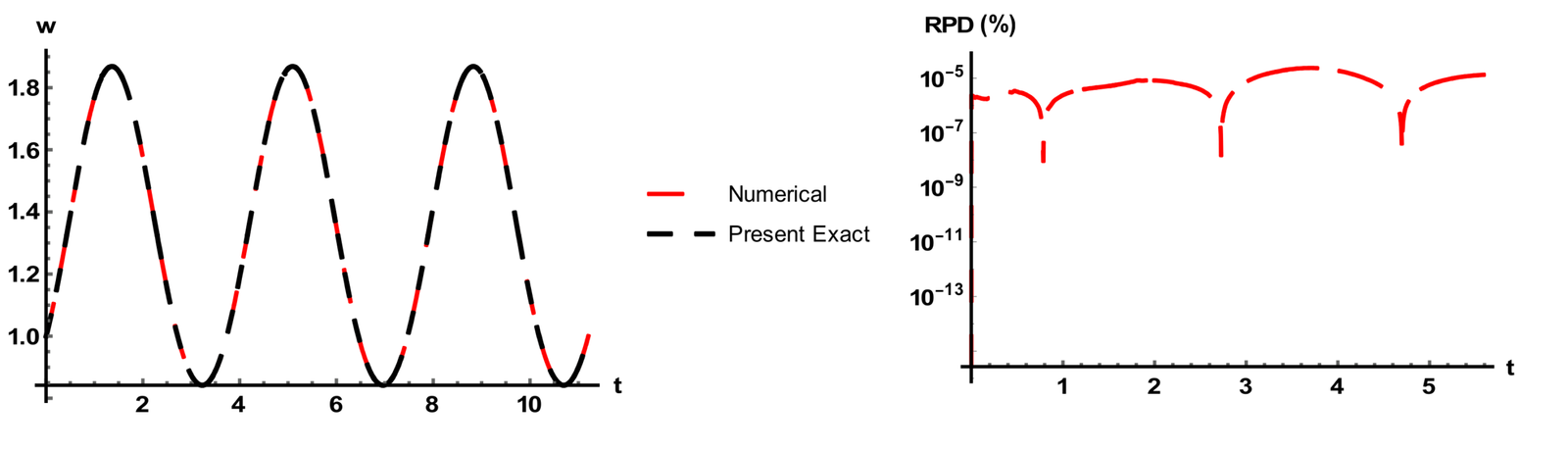
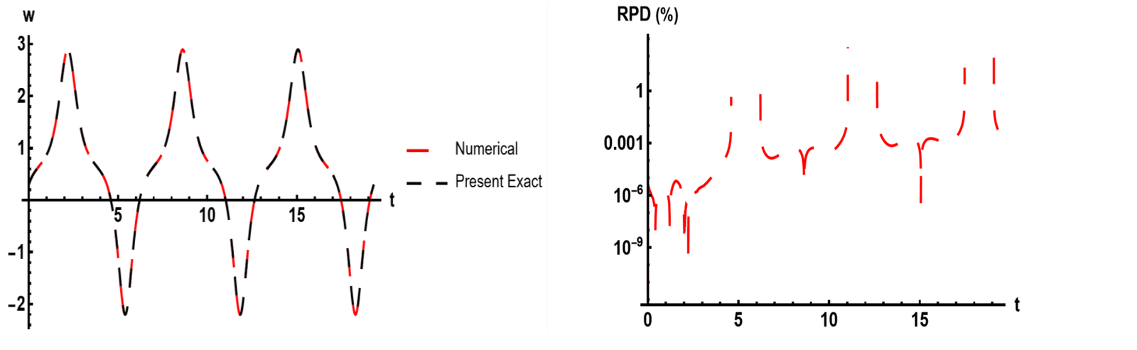
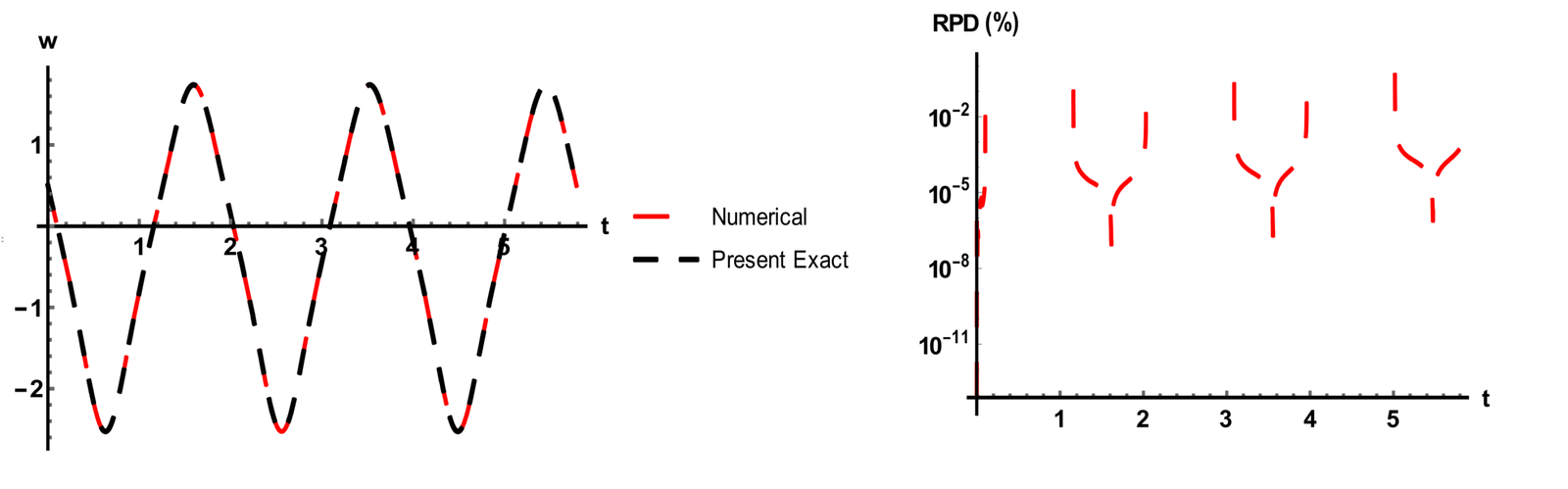
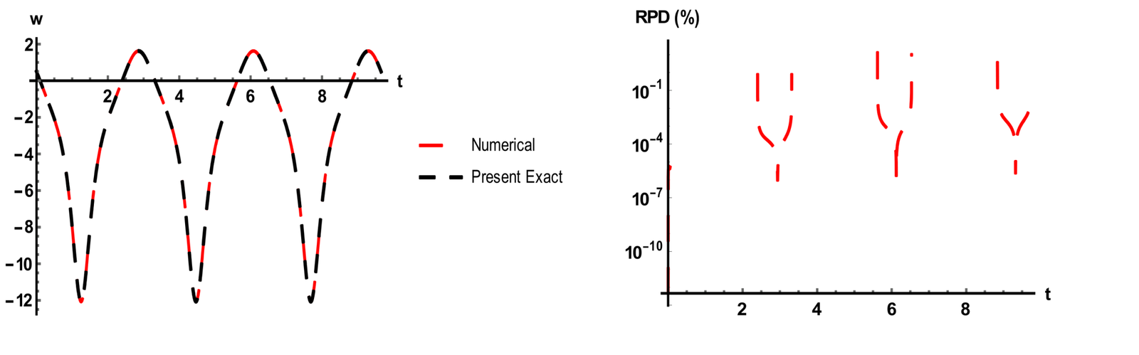
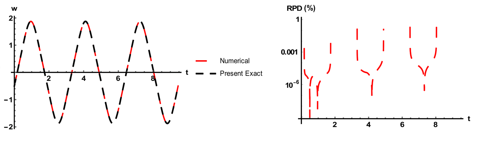
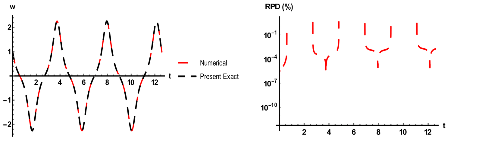
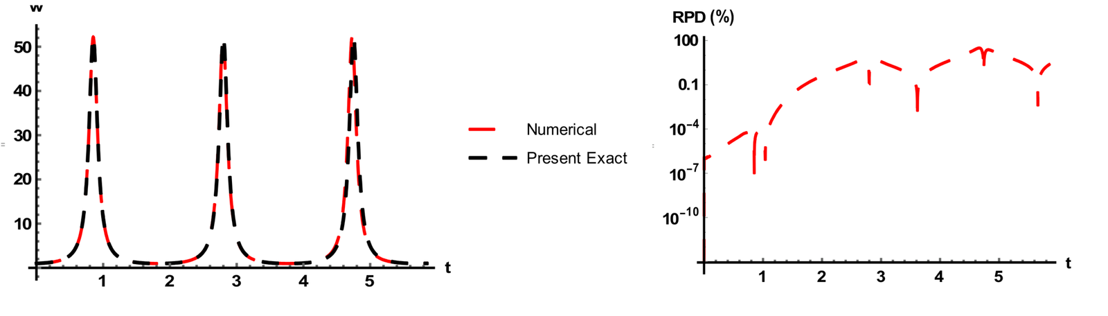
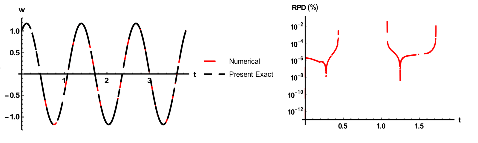
Additionally, the results of the exact displacement were compared with corresponding numerical results for the thirteen different cases as shown in Figures 1 to 13. The discrepancy between the exact and numerical solutions was evaluated using relative percentage difference (RPD) plots. The RPD was calculated as \(100\times|1-w_{num}/w_{ex}|\). Most of the RPD plots show some upward spikes that occur at the zero displacement points. These points are highly sensitive to minor numerical changes and tend to produce significant errors for insignificant differences because of division by a near-zero number when calculating the RPD. The ratio is undefined when \(w_{ex}=0\) and is not a reliable pointwise accuracy measure near a zero crossing. The reported displacement curves generally agree visually, except for some highly nonlinear conditions (e.g., Figures 7 and 12) where the RPD grows with time. Such discrepancies do not establish that the numerical solution is responsible [26]; tolerance refinement, energy and equation residuals, initial-condition checks, and branch-consistent evaluation are needed to identify the source. The figures are retained as reported and have not been regenerated after the algebraic corrections.
To demonstrate the applicability of the equivalent HDO, the periodic response of three pragmatic systems having an asymmetric restoring force defined by a non-polynomial nonlinearity was investigated. The systems considered for the investigation are: a quasi-zero stiffness mass-spring system, ship roll motion, and a rigid flat surface in contact with a deformable rough surface. To assess the accuracy of the equivalent HDO approach for each of the systems, the original restoring force was compared to those of the Taylor series equivalent HDO and quasi-static equivalent HDO. Also, the numerical solution of the original NODE was compared to the exact solution of the equivalent HDO. Two examples described as moderate and strong nonlinear responses were examined for each system. These descriptions refer to the selected cases and do not define a universal measure of nonlinearity or a stability classification.
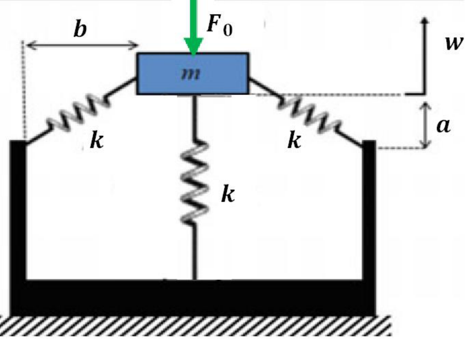
Mass-spring systems find application in many industrial machines and consist of rigid masses that are attached by various spring or elastic member configurations. The quasi-zero stiffness (QZS) mass-spring system considered here consists of a rigid mass attached to a rectangular frame by three springs. In its stationary position, two oblique springs connect the mass to the sides of the frame, and the remaining spring connects the mass vertically to the base. A diagrammatic representation is shown in Figure 14. This QZS mass-spring system has application in energy harvesting [32], vibration isolation [33], and the design of dynamic vibration absorbers [34]. Here QZS identifies the spring arrangement; the selected examples are not shown to meet a zero-tangent-stiffness condition and do not establish isolation or energy-harvesting performance.
The vibration model for the QZS mass-spring system in Figure 14 can be easily derived, and the restoring force is given as [35,36] : \[\tag{41} g(w)=kw+2k(w+a)\left(1-\sqrt{\frac{a^2+b^2}{(a+w)^2+b^2}}\right)-(F_0+mg),\] where \(k\) is the stiffness of the spring, \(a\) and \(b\) are the vertical and horizontal distances of the oblique springs from the mass such that their undeformed length is \(l_0=\sqrt{a^2+b^2}\), \(F_0\) is the constant load, \(m\) is the vibrating mass, and \(g\) is the acceleration due to gravity. In Eqs. (41)–(43c), the restoring force and the polynomial coefficients are written at force level. Before applying the unit-inertia Eqs. (27) and (28), the entire force and all polynomial coefficients must be divided by \(m\); alternatively the inertial term is \(m\ddot w\). The same convention must be used for both approximations and the numerical benchmark.
Based on Taylor’s series expansion of Eq. (41), the equivalent HDO constants are: \[\tag{42a}F=-(F_0+mg),\] \[\tag{42b}k_1=k\left(3-\frac{2b^2}{a^2+b^2}\right),\] \[\tag{42c}k_2=\frac{3kab^2}{(a^2+b^2)^2},\] \[\tag{42d}k_3=\frac{k(b^4-4a^2b^2)}{(a^2+b^2)^3}.\]
On the other hand, the quasi-static equilibrium method produces the following results that were used to compute the stiffness constants in Eqs. (37 – 39). \[\tag{43a}g(0)=-(F_0+mg),\] \[\tag{43b}g(A)=kA+2k(A+a)\left(1-\sqrt{\frac{a^2+b^2}{(a+A)^2+b^2}}\right)-(F_0+mg),\] \[\tag{43c}g(B)=kB+2k(B+a)\left(1-\sqrt{\frac{a^2+b^2}{(a+B)^2+b^2}}\right)-(F_0+mg),\] where the amplitudes \(A\) and \(B\) were obtained from the real roots of \(w_{max}\) in the following equation: \[\begin{gathered} mv_0^2+k(w_0^2-w_{max}^2)-2k(a^2+b^2+2aw_{max}+w_{max}^2)\left(1-2\sqrt{\frac{a^2+b^2}{a^2+b^2+2aw_{max}+w_{max}^2}}\right)\\ +2k(a^2+2aw_0+w_0^2+b^2)\left(1-2\sqrt{\frac{a^2+b^2}{a^2+2aw_0+w_0^2+b^2}}\right) +2(F_0+mg)(w_{max}-w_0)=0. \end{gathered}\tag{44}\]
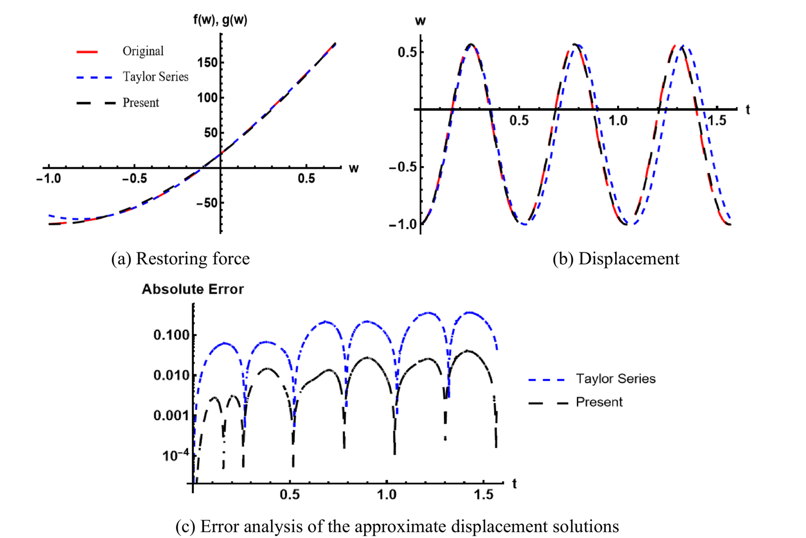
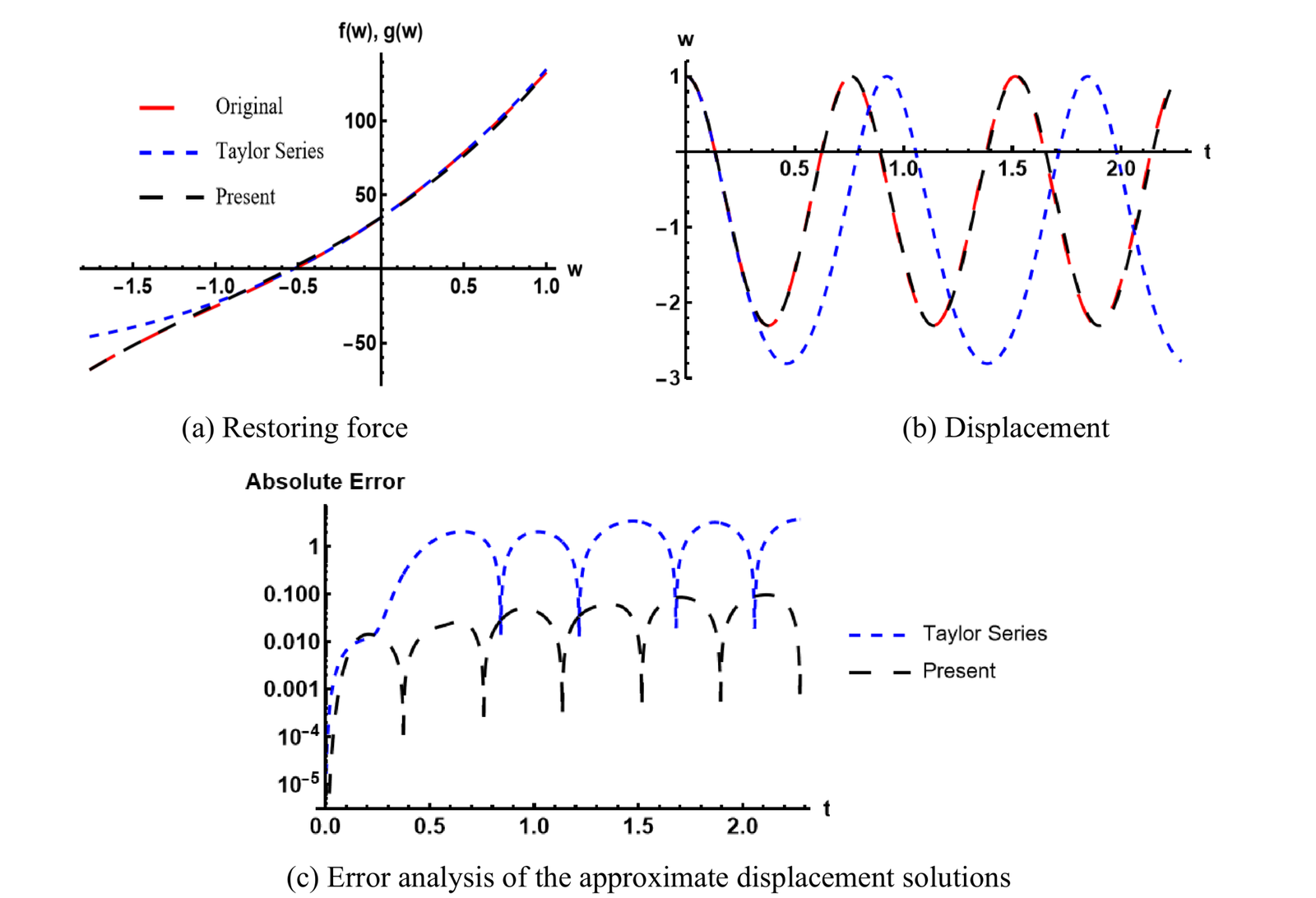
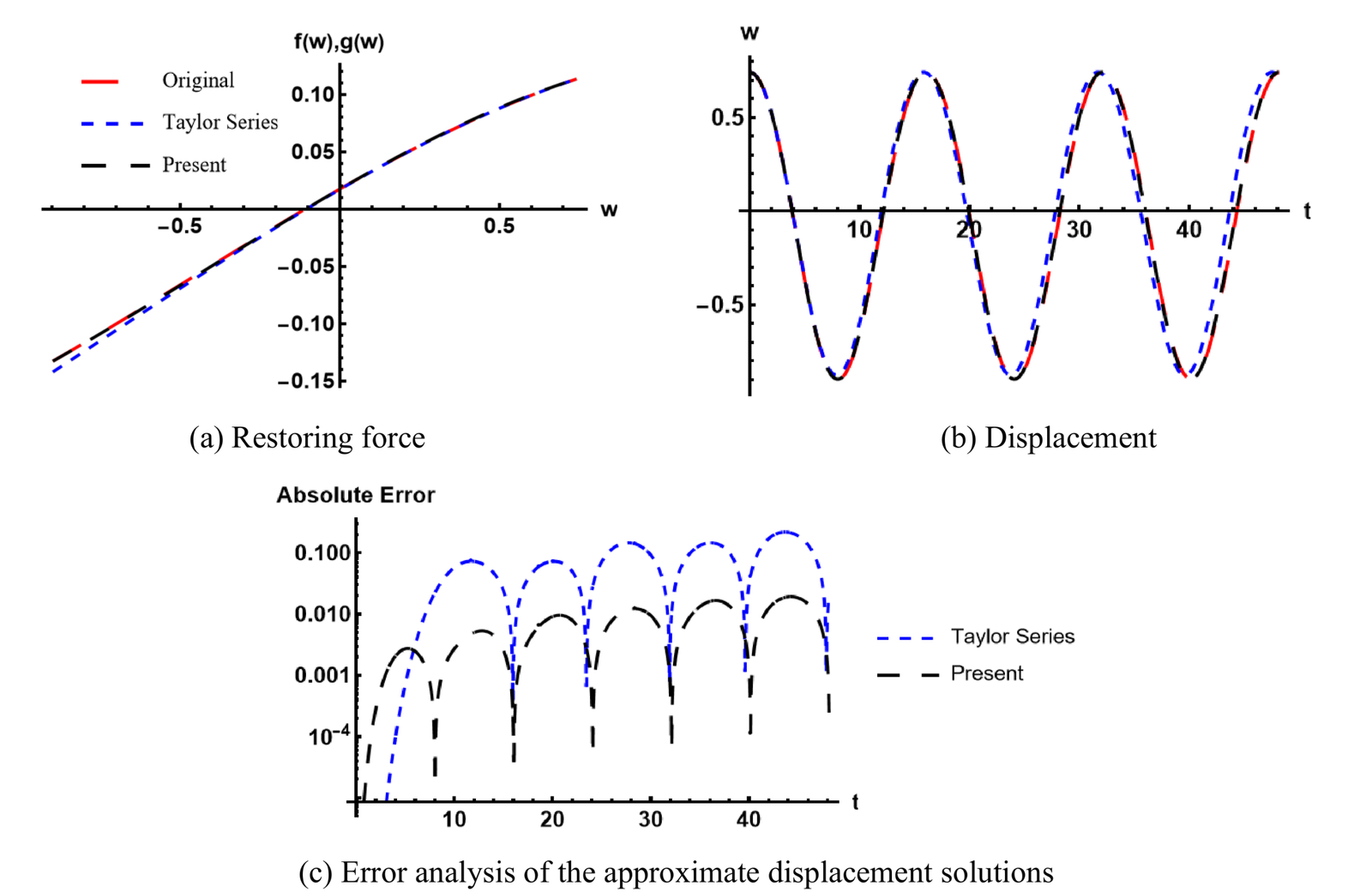
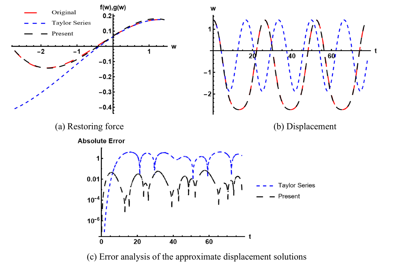
The results for the QZS mass-spring system are summarized in Table 2 and plotted in Figures 15 and 16. The retained numerical records do not specify the signed gravity value or the mass/time normalization used. Figure 16 reports \(F\) rather than \(F_0\), and the implemented conversion between these quantities is not documented. Consequently, the table and figures are reported comparisons, not a revalidation of the mass-normalized model and corrected energy equation.
| Solution method | Moderate nonlinearity | Strong nonlinearity |
|---|---|---|
| Numerical solution of original NODE | 0.522598 | 0.718435 |
| Taylor series equivalent HDO | 0.537896 (2.927%) | 0.948030 (31.958%) |
| Present equivalent HDO | 0.523897 (0.249%) | 0.722776 (0.604%) |
The ship roll motion is an important motion associated with ship capsizes. The restoring force of the large-amplitude roll motion is characterized by righting moment and drag moment, which can lead to asymmetric responses. Big-Alabo and Koroye [37] showed that an amplitude-dependent autonomous representation of the ship roll motion with zero initial velocity and non-zero initial displacement can be derived as: \[\tag{45} g(w)=\frac{D(A)e^{\left(2B_2(A-w)/I_w\right)}-D(w)+C_1w-C_3w^3}{I_w},\] where, \(I_w\) represents the total moment of inertia comprising the ship mass and added mass moments; \(B_2\) is the coefficient of the quadratic nonlinear damping moment; \(C_i\) \((i=1,3)\) are stiffness coefficients whose values can be obtained from an actual GZ-curve; \(A\) is the initial displacement which is one of the amplitudes; \[\tag{46} D(A)=C_1\left(A-\frac{I_w}{2B_2}\right)-C_3\left(A^3-\frac{3I_w}{2B_2}A^2+\frac{3I_w^2}{2B_2^2}A-\frac{3I_w^3}{4B_2^3}\right),\] and \[\tag{47} D(w)=C_1\left(w-\frac{I_w}{2B_2}\right)-C_3\left(w^3-\frac{3I_w}{2B_2}w^2+\frac{3I_w^2}{2B_2^2}w-\frac{3I_w^3}{4B_2^3}\right).\]
The comparisons here concern the autonomous model in Eq. (45) at fixed \(A\) and zero initial angular velocity. They do not establish a periodic solution of a genuinely dissipative roll equation, for which drag removes energy. No capsize threshold or full-scale ship performance is validated by these comparisons. The angles reported in degrees must be converted to radians in the equations, and \(v_0\) is an angular velocity.
Substituting Eq. (47) in (45) and simplifying gives the restoring force as: \[\tag{48} g(w)=\frac{D(A)}{I_w}e^{\left(2B_2(A-w)/I_w\right)}+\frac{3C_3I_w}{2B_2^2}w-\frac{3C_3}{2B_2}w^2+\frac{C_1}{2B_2}-\frac{3C_3I_w^2}{4B_2^3}.\]
The coefficients of the Taylor series equivalent HDO were obtained by expanding the exponential function in Eq. (48) to get: \[\tag{49a} F=\frac{C_1}{2B_2}-\frac{3C_3I_w^2}{4B_2^3}+\frac{D(A)}{I_w}\left(1+\frac{2B_2A}{I_w}+\frac{2B_2^2A^2}{I_w^2}+\frac{4B_2^3A^3}{3I_w^3}\right),\] \[\tag{49b} k_1=\frac{3C_3I_w}{2B_2^2}-\frac{2D(A)B_2}{I_w^2}\left(1+\frac{2B_2A}{I_w}+\frac{2B_2^2A^2}{I_w^2}\right),\] \[\tag{49c} k_2=\frac{2D(A)B_2^2}{I_w^3}\left(1+\frac{2B_2A}{I_w}\right)-\frac{3C_3}{2B_2},\] \[\tag{49d} k_3=-\frac{4D(A)B_2^3}{3I_w^4}.\]
Eqs. (49a)–(49d) truncate the exponential in powers of \(A-w\) about \(w=A\). They are not the Taylor polynomial about \(w=0\). The comparison therefore concerns this specified cubic truncation, not all Taylor-series approximations or an optimized expansion point.
The coefficients of the quasi-static equivalent HDO were computed using Eqs. (37 – 40a–h) and the following results: \[\tag{50a} g(0)=\frac{D(A)e^{(2B_2A/I_w)}}{I_w}+\frac{C_1}{2B_2}-\frac{3C_3I_w^2}{4B_2^3},\] \[\tag{50b} g(A)=\frac{D(A)}{I_w}+\frac{3C_3I_w}{2B_2^2}A-\frac{3C_3}{2B_2}A^2+\frac{C_1}{2B_2}-\frac{3C_3I_w^2}{4B_2^3},\] \[\tag{50c} g(B)=\frac{D(A)}{I_w}e^{(2B_2(A-B)/I_w)}+\frac{3C_3I_w}{2B_2^2}B-\frac{3C_3}{2B_2}B^2+\frac{C_1}{2B_2}-\frac{3C_3I_w^2}{4B_2^3}.\]
Finally, the biased amplitude (\(B\)) of the asymmetric vibration of the ship roll motion was derived from the nontrivial root on the same bounded energy interval of the following nonlinear equation. \[\tag{51} D(A)e^{(2B_2(A-B)/I_w)}-C_1\left(B-\frac{I_w}{2B_2}\right) +C_3\left(B^3-\frac{3I_w}{2B_2}B^2+\frac{3I_w^2}{2B_2^2}B-\frac{3I_w^3}{4B_2^3}\right)=0.\]
The root \(B=A\) is the initial turning point and is excluded when selecting the distinct biased amplitude. The results for the vibration response of the ship roll motion are given in Table 3 and Figures 17 and 18.
| Solution method | Moderate nonlinearity | Strong nonlinearity |
|---|---|---|
| Numerical solution of original NODE | 16.069281 | 26.133033 |
| Taylor series equivalent HDO | 15.844339 (1.400%) | 16.605956 (36.456%) |
| Present equivalent HDO | 16.047362 (0.136%) | 26.112896 (0.077%) |
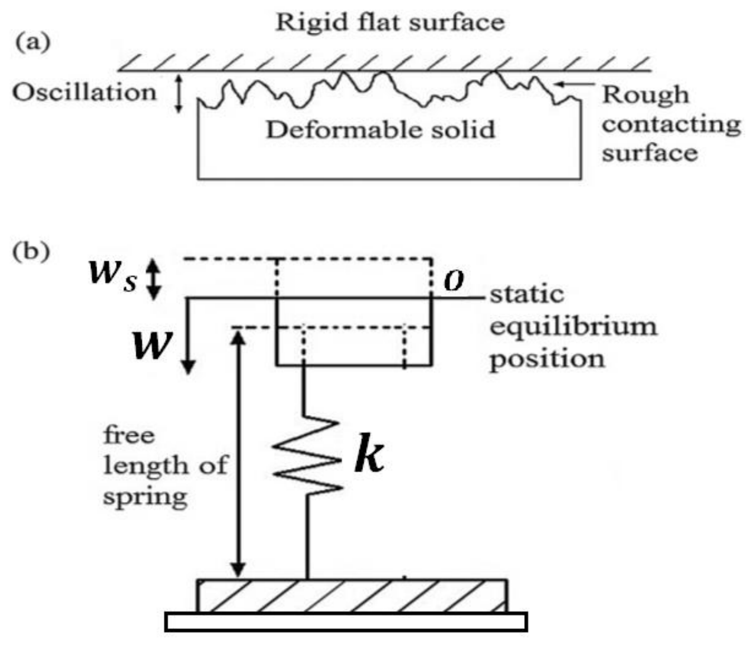
The vibration of a rigid flat surface in contact with a deformable rough surface is illustrated in Figure 19 and can be modelled as [38] : \[\tag{52} \ddot w+\frac1n[(w+1)^n-1]=\frac{F_0}{nmg}\cos(\alpha\tau),\]
The undamped vibration of the system in Figure 19 subjected to a constant force can be obtained by setting \(\alpha=0\). The resulting equation is given as: \[\tag{53} \ddot w+\frac1n[(w+1)^n-1]+F_1=0,\] where \(n>0\), \(F_1=-F_0/(nmg)\), \(F_0\) is the dimensional constant load, and the restoring force is: \[\tag{54} g(w)=\frac1n[(w+1)^n-1]+F_1.\]
Here the dots refer to the normalized time \(\tau\), and the load normalization in Eq. (52) is the same as in Eq. (53). For noninteger \(n\), the real contact law requires \(w+1\ge0\). Only trajectories that remain in this contact domain are considered; no separation or impact rule is included. An approximate trajectory leaving this domain cannot be interpreted as a valid real contact response.
The coefficients of the equivalent HDO based on Taylor series expansion of the restoring force are: \(k_1=1\), \(k_2=(n-1)/2\), \(k_3=(n-1)(n-2)/6\) and \(F=F_1\). For the equivalent HDO based on the quasi-static equilibrium approach, the coefficients were obtained by using the following results and Eqs. (37 – 40a–h). \[\tag{55a}g(0)=F_1,\] \[\tag{55b}g(A)=\frac1n[(A+1)^n-1]+F_1,\] \[\tag{55c}g(B)=\frac1n[(B+1)^n-1]+F_1.\]
Given that the initial conditions are \(w(0)=w_0\) and \(\dot w(0)=v_0\), the amplitudes \(A\) and \(B\) were determined from the real roots of \(w_{max}\) in the following equation: \[\tag{56} v_0^2-\frac{2}{n(n+1)}[(w_{max}+1)^{n+1}-(w_0+1)^{n+1}]+2\left(\frac1n-F_1\right)(w_{max}-w_0)=0,\]
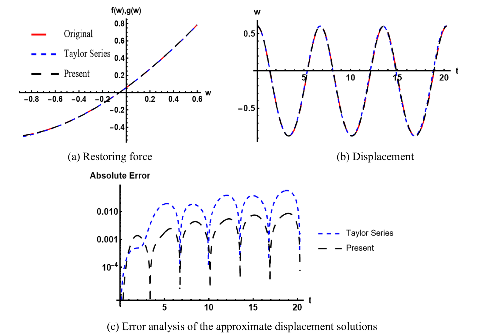
The results for the vibration response of the rigid flat surface in contact with a deformable rough surface are summarized in Table 4 and plotted in Figures 20 and 21. The captions do not specify \(v_0\), and the conversion from the listed \(k,m\) to normalized time is not provided. The numerical comparisons therefore cannot be independently reproduced as fully specified initial-value problems, and the tabulated periods are not assigned physical time units. The \(F\) in these captions equals \(F_1\) through Eq. (33).
| Solution Method | Moderate nonlinearity | Strong nonlinearity |
|---|---|---|
| Numerical solution of original NODE | 6.765654 | 8.537578 |
| Taylor series equivalent HDO | 6.738562 (0.400%) | 6.622996 (22.425%) |
| Present equivalent HDO | 6.761078 (0.068%) | 8.556953 (0.227%) |
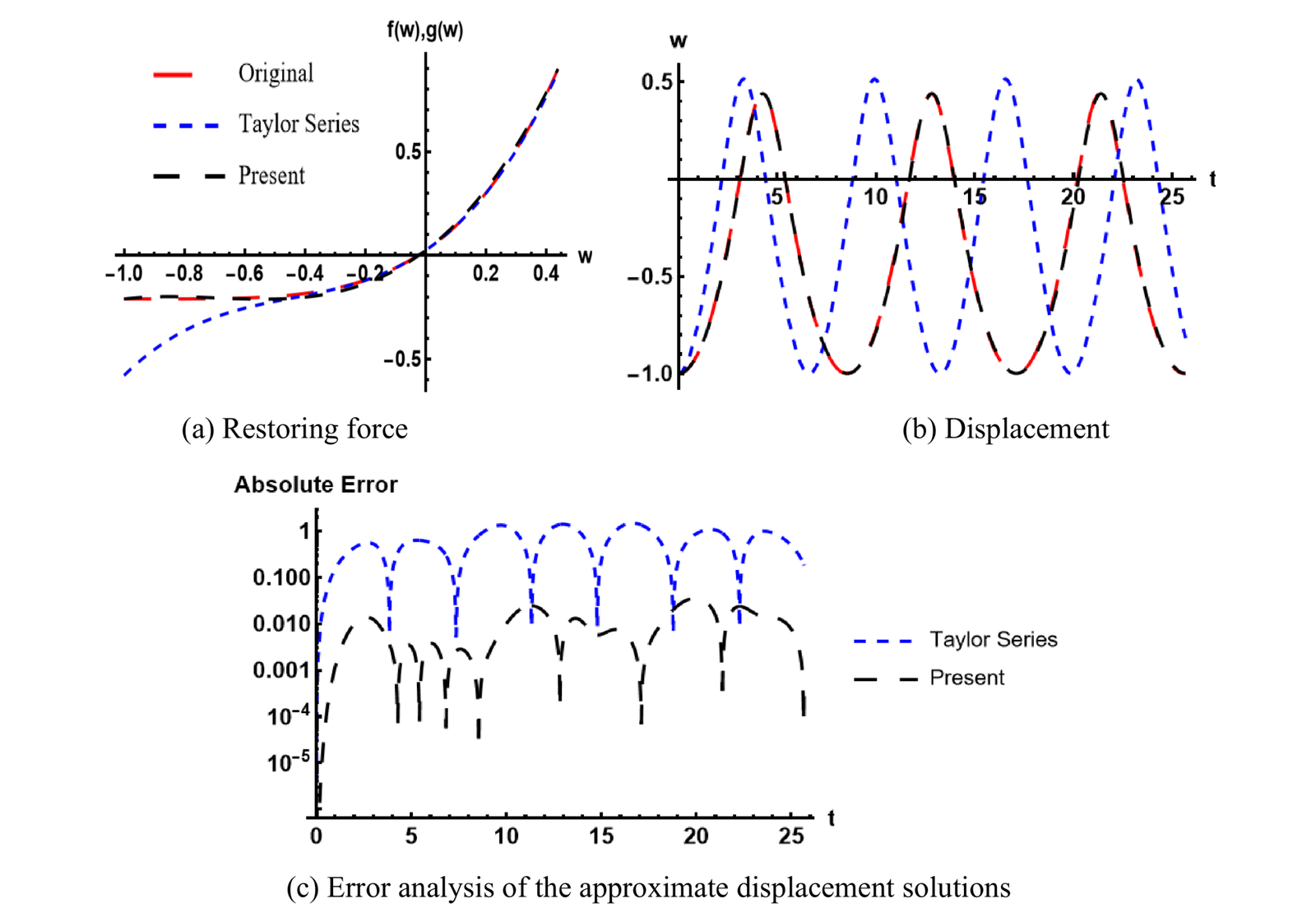
The results shown in Figures 15 to 18, 20 and 21 compare the original restoring force and reported numerical displacement response with the corresponding approximate solutions of the Taylor series equivalent HDO and the quasi-static equivalent HDO. Three asymmetric oscillator models with non-polynomial nonlinearities were simulated in these Figures, namely: the QZS mass-spring system (Figures 15 and 16), ship roll motion (Figures 17 and 18), and vibration of a rigid flat surface in contact with a deformable rough surface (Figures 20 and 21). For each asymmetric oscillator, conditions described as moderate nonlinearity (Figures 15, 17 and 20) and strong nonlinearity (Figures 16, 18 and 21) were simulated. Under conditions of moderate nonlinearity, the plotted Taylor approximation only shows a minor deviation from the original restoring force around the biased amplitude, whereas a significant deviation is seen in the case of strong nonlinearity. The reported quasi-static curves are closer to the original restoring force over the plotted ranges. Similar trends are reported for the displacement response and time period estimates as shown in Tables 2 to 4. The absolute-error panels compare \(|w_{approx}-w_{num}|\) over the displayed time intervals; they do not establish an all-time displacement-error bound. Note that the percentages in brackets represent the absolute relative error of the equivalent HDO in estimating the time period, i.e. \(100\times|1-T_{HDO}/T_{num}|\%\). These reported comparisons favour the quasi-static approximation for the selected cases, subject to the reproducibility and domain limitations stated above. Because the quasi-static construction uses two turning points while the Taylor approximations use local expansion data, the comparisons do not establish general superiority at equal computational cost. No convergence study, uniform error bound, or runtime comparison is reported.
Many studies have developed approximate analytical methods to provide solutions to nonlinear vibration models. Several methods discussed here address nonlinear symmetric vibrations, while other methods also solve nonlinear asymmetric vibration models. Limitations relevant to the present comparison include: (a) some methods require polynomial series approximation when the stiffness nonlinearities are expressed in terms of non-polynomial functions, (b) some published formulations use restricted initial conditions, and (c) fixed low-order approximations can lose accuracy under strong nonlinear vibration. These limitations are not asserted for every existing method.
In this paper, we propose an equivalent HDO for approximate periodic solutions of nonlinear asymmetric oscillators with non-polynomial nonlinearity. The present approach is based on the use of the quasi-static equilibrium principle to develop the constants in the equivalent HDO and then applying the exact analytical solution of an HDO with generalized initial conditions and constant load to obtain an approximate solution of the original NODE. The contribution is the mixed-parity force-and-energy matching construction within the established equivalent-oscillator framework, together with a consistent initial-phase prescription. Its use requires admissible bounded initial states, nonsingular matching coefficients, and a valid equivalent oscillation interval. The reported comparisons for typical asymmetric oscillators favour the present approximation over the specified cubic Taylor approximations, including the selected strongly nonlinear cases. However, inconsistent entries in Table 1, incomplete numerical settings, and unresolved normalization and initial-condition details prevent a general validation or an unconditional accuracy claim. The reported values and plots have not been regenerated after the mathematical corrections. Accordingly, the study supports an amplitude-dependent approximation framework rather than universal robustness, superiority to all Taylor methods, or a demonstrated computational-efficiency gain. Additionally, it provides a way of interpreting the selected nonlinear asymmetric models using a simpler equivalent model, subject to the operating-domain and validation limitations stated above.
Author Contributions: All authors contributed equally to the conception, development, and preparation of the manuscript. All authors have read and approved the final version of the manuscript for publication.
Conflicts of Interest: The authors declare that there are no conflicts of interest related to this work.
Data Availability: No datasets were generated or analyzed during the present study; therefore, data availability is not applicable.
Funding Information: This research received no external funding.
First, the following constants are defined. \[\alpha=-\frac{3a_3^2}{8}-a_2,\tag{A1}\]\[ \tag{A2}\beta=-\frac{a_3^3}{8}-\frac{a_3a_2}{2}-a_1,\]\[ \tag{A3}\gamma=-\frac{3a_3^4}{256}-\frac{a_2a_3^2}{16}-\frac{a_3a_1}{4}-a_0,\]\[ \tag{A4}p=-\frac{\alpha^2}{12}-\gamma,\]\[ \tag{A5}q=-\frac{\alpha^3}{108}+\frac{\alpha\gamma}{3}-\frac{\beta^2}{8},\]\[ \tag{A6}r=\left(-\frac q2+\sqrt{\frac{q^2}{4}+\frac{p^3}{27}}\right)^{1/3},\]\[ \tag{A7} y=\begin{cases}\operatorname{Re}\left(-\frac{5\alpha}{6}+r-\frac{p}{3r}\right),r\ne0,\\ \operatorname{Re}\left(-\frac{5\alpha}{6}-\sqrt[3]{q}\right),r=0.\end{cases}\]\[ \tag{A8}\mu=\sqrt{\alpha+2y}.\]
Thereafter, the real roots of the quartic equation in Eq. (7) can be determined based on the values of \(D=\operatorname{Re}(3\alpha+2y+2\beta/\mu)\), \(\beta\) and \(k_3\) as follows. For \(\beta\ne0\), the cube-root branch in Eq. (A6) must give a real resolvent value \(y\) and a nonzero real \(\mu\); the real-part notation in Eq. (A7) is not permission to discard a genuine imaginary component. The formulas below generate candidate roots. In every case, retain real roots satisfying Eq. (7), order them, and select the adjacent pair enclosing \(w_0\) for which the first-integral radicand is positive throughout the interior. A pair that crosses another real root or lies on an escaping component is not an admissible oscillation interval. Repeated-root and singular-resolvent limits are excluded from direct use of these case formulas.
Case 1; \(\boldsymbol{D<0,\ k_3>0\ \&\ \beta\ne0}\) \[\tag{A9} (w_1,w_2)=(\rho_i,\rho_j),\qquad \rho_i>\rho_j,\qquad w_0\in[\rho_j,\rho_i].\]
Here \(\rho_i,\rho_j\) are adjacent real candidates subject to the interior-positivity condition just stated. Their signs alone do not determine the correct potential well.
Case 2: \(\boldsymbol{D<0,\ k_3<0\ \&\ \beta\ne0}\) \[\tag{A10} w_1,w_2=\rho_{(2)},\rho_{(3)},\] where \(\rho_{(1)}>\rho_{(2)}>\rho_{(3)}>\rho_{(4)}\) denotes the four real roots in descending order, independently of their formula indices. The bounded orbit must contain \(w_0\) between the middle two roots.
Case 3: \(\boldsymbol{D>0\ \&\ \beta\ne0}\) \[\tag{A11} w_1,w_2=\frac{a_3}{4}-\frac{\mu\mp\sqrt{-(3\alpha+2y-2\beta/\mu)}}{2}.\]
This pair is used only when it is real and satisfies the same bounded-interval condition.
Case 4: \(\boldsymbol{k_3>0\ \&\ \beta=0}\) \[\tag{A12} \rho_1,\rho_4=\frac{a_3}{4}\pm\sqrt{\frac{-\alpha+\sqrt{\alpha^2-4\gamma}}{2}}.\]
Case 5: \(\boldsymbol{k_3<0\ \&\ \beta=0}\) \[\tag{A13} \rho_2,\rho_3=\frac{a_3}{4}\pm\sqrt{\frac{-\alpha-\sqrt{\alpha^2-4\gamma}}{2}}\]
For \(\beta=0\), Eqs. (A12) and (A13) together generate the biquadratic candidates, for either sign of \(k_3\). Only real candidates are retained, and Eq. (A9) selects the oscillation interval. In particular, a \(k_3>0\) orbit confined to one well cannot be assigned the two outer roots solely from Eq. (A12).
For \(\beta\ne0\), the four Ferrari candidates used above are \[\tag{A14} \rho_1,\rho_2=\frac{a_3}{4}+\frac{\mu\pm\sqrt{-(3\alpha+2y+2\beta/\mu)}}{2},\] \[\tag{A15} \rho_3,\rho_4=\frac{a_3}{4}-\frac{\mu\mp\sqrt{-(3\alpha+2y-2\beta/\mu)}}{2}.\]
Geng (2015) applied the following discriminants and constants to determine the conditions for bounded periodic oscillations of the HDO. \[ \tag{B1}\Delta_1=3k_1k_3-k_2^2,\]\[ \tag{B2}\Delta_2=9k_1k_2k_3-27Fk_3^2-2k_2^3,\]\[ \tag{B3}\Delta_3=k_1^2k_2^2+18k_1k_2k_3F-27F^2k_3^2-4Fk_2^3-4k_1^3k_3,\]\[ \tag{B4}\Delta_4=k_2^2-4k_1k_3,\]\[ \tag{B5}c_1=-\Delta_2/(3k_3\Delta_1),\]\[ \tag{B6}c_2=\Delta_2/(6k_3\Delta_1).\]
The constants \(c_1,c_2\) in Eqs. (B5) and (B6) are the repeated-root values in the depressed cubic coordinate when \(\Delta_3=0\) and \(\Delta_1\ne0\). They are not general equilibrium roots; the corresponding original coordinate is \(w=c_j-k_2/(3k_3)\). Their singular cases require separate treatment. \[\tag{B7} w_{01}=(-k_2+\sqrt{\Delta_4})/(2k_3),\]\[\tag{B8} w_{02}=(-k_2-\sqrt{\Delta_4})/(2k_3).\]
Eqs. (B7) and (B8) give the nonzero equilibrium candidates for \(F=0\), with \(k_3\ne0\) and \(\Delta_4\ge0\).
Additionally, the Hamiltonian function was applied as follows: \[\tag{B9} h=h(w,v)=\frac12v^2+Fw+\frac{k_1}{2}w^2+\frac{k_2}{3}w^3+\frac{k_3}{4}w^4,\] \[\tag{B10}h_0=h(0,0)=0,\] \[\tag{B11} h_i=h(w_i,0)=Fw_i+\frac{k_1}{2}w_i^2+\frac{k_2}{3}w_i^3+\frac{k_3}{4}w_i^4,\] \[\tag{B12} h_{0j}=h(w_{0j},0)=Fw_{0j}+\frac{k_1}{2}w_{0j}^2+\frac{k_2}{3}w_{0j}^3+\frac{k_3}{4}w_{0j}^4,\] where \(w_i\) (for \(i=I,II,III\)) are the real equilibrium roots of \(k_1w+k_2w^2+k_3w^3+F=0\) which can be obtained analytically (Big-Alabo and Alfred, 2025), and \(w_{0j}\) (for \(j=1,2\)) are defined in Eqs. (B7) and (B8). At least one equilibrium root is real; the other two can be real or complex. For three real equilibria, take \(w_I>w_{II}>w_{III}\); the \(h_1,h_3\) used in Table 1 and the associated captions denote \(h_I,h_{III}\) in this ordering. These equilibrium roots are distinct in meaning from the turning-point roots used in §2. An energy interval and the appropriate local potential well must also be specified: discriminant signs alone do not establish a bounded orbit for arbitrary initial conditions, and bounded periodic motion does not imply asymptotic stability in this undamped system.