
Hydrology deals with the comprehensive study of the earth’s water, focusing on its occurrence, movement, distribution, and the intricate chemical and physical properties that govern its interactions with the environment, particularly its relationships with living organisms [1]. A critical aspect of hydrology is surface runoff, which occurs when rainfall exceeds the soil’s infiltration capacity or when the soil becomes saturated, causing excess water to flow over the land surface into nearby waterways such as rivers, streams, reservoirs, and lakes [2]. The significance of surface runoff extends to water resource monitoring and the management of water quality and quantity, addressing issues such as flood predictions and the ecological impacts on aquatic environments [3].
The dynamics of hydrologic systems have been profoundly influenced by rapid urbanization, which includes factors such as deforestation, land cover changes, industrialization, and irrigation practices [4]. Furthermore, climate change and soil variability have been shown to significantly affect surface runoff and river flow patterns at the global scale. Understanding the implications of runoff pollution is essential for water managers, as it enables the implementation of preventive measures to safeguard water resources. Consequently, runoff modeling has become an essential tool for understanding and predicting hydrological processes and watershed responses to environmental and climatic changes [5,6]. Moreover, runoff plays a critical role in the transport of contaminants, as excess nutrients, fertilizers, and pesticides from agricultural lands are often carried into rivers and other surface water bodies during runoff events [7,8].
The relationship between rainfall and runoff from a given drainage basin is influenced by numerous interrelated factors, including the basin’s shape, size, slope, vegetative cover, and the duration and frequency of rainfall events, all of which directly impact peak flow and runoff volume [9,10]. Poor drainage systems within catchment areas are often the primary contributors to runoff generation, while improper solid waste disposal can lead to the blockage of waterways [11,12]. Risk assessments related to runoff are typically conducted using remote sensing, geographic information systems (GIS), and various modeling techniques [13]. In cases where data is scarce, ungauged watersheds are often modeled using empirical methods [14,15].
Runoff generation results primarily from two mechanisms: infiltration- and saturation-excess runoff [16]. The runoff method, originally developed by Thomas Mulvaney in 1851, serves to determine the drainage area, rainfall intensity, and runoff coefficient necessary for calculating peak discharge [17,18]. The unit hydrograph concept was introduced to conceptualize a catchment’s response to specific storm events based on the superposition principle [19,20]. Runoff models are instrumental in visualizing hydrological system responses to changes in vegetation cover, pervious surfaces, and meteorological events [21,22]. These models are utilized to analyze catchment yields and responses, track changes over time, make forecasts, and estimate water availability.
Conventional hydrologic frequency analysis generally assumes that historical rainfall records are stationary, implying that the statistical properties of rainfall remain constant over time. However, climate variability and land-use changes may introduce trends or shifts in rainfall extremes, potentially affecting the reliability of design rainfall estimates. Despite these concerns, the assumption of stationarity remains widely adopted where long-term records do not exhibit statistically significant temporal changes or where the objective is to support engineering design based on historical observations.
The conversion of rainfall into runoff is a complex hydrological process influenced by rainfall characteristics, catchment properties, soil conditions, land use, and antecedent moisture. Nevertheless, several empirical and statistical methods have been developed to estimate design runoff with acceptable accuracy for engineering applications. In this study, the annual maximum rainfall series was assumed to be stationary for frequency analysis using the Log-Pearson Type III distribution. Consequently, the derived design rainfall and runoff estimates represent historical climatic conditions and should be interpreted cautiously when applied to future infrastructure planning under changing climate conditions.
Among the methods applied, the Win-TR-20 computer model, developed by the Natural Resources Conservation Service (NRCS) in 1964, is specifically designed for hydrologic studies of storm water. The Win-TR-20 software is characterized by its user-friendly interface and simplicity, making it a popular choice for evaluating peak runoff volumes [23]. The model has been tested in various contexts, including simulations of runoff hydrographs in ungauged rural watersheds in Korea [24] and calculations of flood hydrographs in the Dreisam watershed in southwestern Germany [25]. Additionally, Win-TR-20 has been applied to both agricultural and urban watersheds for storm runoff predictions [26].
Although rainfall–runoff modeling and flood frequency analysis have been widely applied using statistical distributions such as the Log-Pearson Type III (LP-III) distribution and hydrological simulation models, many studies focus primarily on large river basins or flood forecasting without integrating statistical rainfall frequency analysis with hydrological modeling for canal systems in semi-arid regions. In addition, the applicability of combined LP-III frequency analysis and hydrological models for estimating peak runoff and canal discharge in data-limited regions such as Peshawar, Pakistan, remains insufficiently explored. Existing studies also highlight uncertainties in hydrological model validation and parameter estimation, which can affect runoff projections and water resource planning [27].
This study aims to address the existing research gap by estimating design rainfall, generate design-storm hydrographs, and simulate peak runoff for the ungauged Narai Canal catchment in Peshawar, Khyber Pakhtunkhwa, Pakistan, using the Log-Pearson Type III (LP-III) distribution and the WinTR-20 hydrologic model. Specifically, the study sought to (i) estimate one-day design rainfall for selected return periods using the LP-III distribution, (ii) simulate runoff hydrographs and peak discharges using the Soil Conservation Service (SCS) curve number method implemented in WinTR-20, and (iii) provide preliminary hydrological information to support canal hydraulic design, drainage planning, and flood-risk assessment in the absence of observed streamflow records.
Peshawar, located in Khyber Pakhtunkhwa, Pakistan, exhibits a unique climatic pattern compared to other regions of the country, as it does not fall within the monsoon belt. Rainfall in Peshawar occurs during both the winter and summer seasons, with distinct characteristics attributed to each period [28]. The winter months, particularly from February to April, experience the highest levels of precipitation, primarily due to western disturbances. Notably, the maximum winter rainfall recorded in Peshawar was 236 mm in February 2007. In contrast, the summer season also contributes significantly to the region’s hydrology, with the highest summer rainfall reaching 402 mm in July 2010. A remarkable rainfall event occurred on 29 July 2010, when a maximum 24-h point rainfall of 294 mm was recorded at the meteorological station, exceeding the previous record of 187 mm observed in April 2009. This value represents the station-based maximum rainfall and characterizes the severity of the storm. Analyzing the overall rainfall patterns, winter rainfall levels tend to be higher than those observed in the summer months. A comprehensive assessment of a 30-year rainfall record indicates that the average annual precipitation in Peshawar is approximately 400 mm (16 inches). The region has experienced its highest annual rainfall of 904.5 mm during the Kharif and Rabi seasons, as reported by the Pakistan Meteorological Department, Peshawar, [29]. Understanding these rainfall dynamics is crucial for assessing the rainfall-runoff relationship, which is the focus of this study, as it informs water resource management and flood risk assessment in the canal system of Peshawar.
The study was conducted along the Narai Canal system in Peshawar District, Khyber Pakhtunkhwa, Pakistan. The investigated canal reach extends from Ring Road, Hayatabad, to Lalazar Colony near the University of Agriculture Peshawar, approximately between 33.96°–34.01° N and 71.42°–71.47° E (Figure 1). These coordinates define the mapped canal corridor used for field investigations and hydraulic analysis and do not represent the full extent of the contributing runoff catchments.
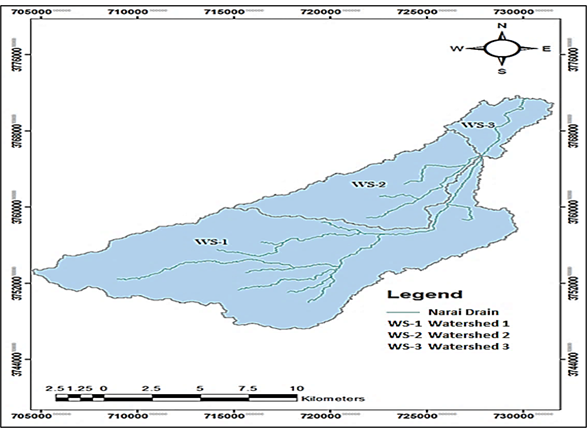
For hydrological analysis, the drainage area contributing runoff to the study reach was delineated from a digital elevation model (DEM) and subdivided into three sub-catchments corresponding to Narai Canal Upper, Narai Canal Lower, and Regi Canal. The combined contributing watershed area is approximately 255.1 \(km^{2}\), whereas the coordinate bounds represent only the location of the canal segment within the larger drainage system.
The study area experiences seasonal high-intensity rainfall that, together with limited urban drainage capacity, frequently causes localized flooding and overtopping of canal sections, resulting in damage to nearby residential areas. Therefore, rainfall–runoff modelling using the LP-III distribution and the WinTR-20 model was undertaken to estimate design runoff and support flood mitigation and canal management in the study area.
The rainfall–runoff analysis was carried out using the USDA NRCS WinTR-20 model to simulate peak runoff and runoff hydrographs for return periods of 2, 5, 10, 25, 50, 100, and 200 years. A 30 m Digital Elevation Model (DEM) was used to delineate the Narai Canal catchment, derive drainage characteristics, and estimate watershed parameters required for the WinTR-20 model. Catchment boundaries and drainage networks were extracted using standard GIS hydrological tools.
Land-use/land-cover (LULC) information was derived from a 10 m SPOT multispectral image. Before classification, the image was subjected to geometric correction, radiometric correction, and sub-setting to the area of interest (AOI). A supervised classification was performed in ERDAS Imagine using the Maximum Likelihood Classifier (MLC), which is widely applied in watershed studies because of its robust statistical performance. Representative training samples for each land-use class were selected from field observations and high-resolution satellite imagery. The final classification included 4 land-use classes (e.g., agriculture, rangeland, built-up, and exposed rocks), which were subsequently used to assign NRCS Curve Number (CN) values for runoff estimation.
Classification accuracy was evaluated using an independent set of 200 validation samples (50 samples per land-use class) and a confusion matrix. The overall accuracy, producer’s accuracy, user’s accuracy, and Cohen’s kappa coefficient were computed following standard remote-sensing accuracy assessment procedures. The classified LULC map and associated uncertainty were considered during CN assignment because classification errors may propagate into runoff estimates.
The rainfall data corresponding to a given return period constitute a critical input for the WinTR-20 hydrological model for estimating peak runoff under different storm events. A total of 41 annual maximum daily rainfall (AMDR) observations (1985–2025) were obtained from the Pakistan Meteorological Department (PMD) and used for rainfall frequency analysis. The dataset was subjected to quality control to identify missing values, inconsistencies, and outliers. No missing values were detected, and the identified outliers were retained because they represented actual extreme rainfall events. Consistent with the assumptions of conventional hydrologic frequency analysis, the AMDR series was assumed to be stationary; therefore, no formal statistical tests for temporal trends or change points were performed. Consequently, the estimated design rainfall values represent historical climatic conditions and should be interpreted with caution under changing climate conditions. The quality-controlled rainfall series was analyzed using EasyFit software, and candidate probability distributions were evaluated using the Chi-square goodness-of-fit test. Among the tested distributions, the Log-Pearson Type III (LP-III) distribution provided the best fit to the observed data and was subsequently used to estimate design rainfall for the selected return periods. The resulting design rainfall depths were then used as inputs to the WinTR-20 model for runoff simulation.
The Log-Pearson Type III (LP-III) distribution was used to estimate design rainfall corresponding to selected return periods. Let Pi denote the annual maximum daily rainfall for year i, and let \[Y_{i} = \log_{10}(P_{i}),\] represent its base-10 logarithm, where \(i = 1, 2, \ldots, N\) and \(N\) is the number of annual observations.
The sample mean, standard deviation, and coefficient of skewness of the logarithmically transformed rainfall data were calculated as follows: \[\overline{Y} = \frac{1}{N}\sum\limits_{i=1}^{N}Y_{i},\tag{1}\] \[s_{Y} = \left[ \frac{1}{N-1}\sum\limits_{i=1}^{N}(Y_{i}-\overline{Y})^{2} \right]^{1/2},\tag{2}\] \[G_{Y} = \frac{N}{(N-1)(N-2)}\sum\limits_{i=1}^{N}\left(\frac{Y_{i}-\overline{Y}}{s_{Y}}\right)^{3},\tag{3}\] where \(\overline{Y}\) is the mean of the logarithmic rainfall values \(s_{Y}\) is the sample standard deviation, and \(G_{Y}\) is the sample coefficient of skewness. The logarithmic rainfall corresponding to a return period T was computed as \[Y_{T} = \overline{Y} + K_{T}\left(G_{Y}\right)s_{Y}\tag{4}\] where \(K_{T}\) is the frequency factor corresponding to the return period T and the sample skewness \(G_{Y}\). The design rainfall was then obtained by back-transforming the logarithmic value as \[P_{T} = 10^{V_{T}},\tag{5}\] where \(P_{T}\) is the estimated rainfall associated with the return period T. In this study, rainfall depths were estimated for return periods of 2, 5, 10, 25, 50, and 100 years using the LP-III distribution.
The Soil Conservation Service Curve Number (SCS-CN) method was used to estimate the direct runoff depth from rainfall, while the resulting runoff hydrograph and peak discharge were generated using WinTR-20 (Fig. S2). The SCS-CN method estimates direct runoff as a depth rather than a discharge and is expressed as:
\[Q_{d} = \frac{(P-I_{a})^{2}}{P+I_{a}+S}, \qquad p > I_{a},\tag{6}\]
\[Q_{d} = 0, \qquad p \leq I_{a},\tag{7}\] where \(Q_{d}\) is the direct runoff depth (mm), \(P\) is the rainfall depth (mm), \(I_{a}\) is the initial abstraction (mm), and \(S\) is the potential maximum retention (mm). Assuming the conventional value of \(\lambda=0.2\), where \(I_{a}=\lambda S\), Eq. (6) becomes: \[Q_{d} = \frac{(P-0.2S)^{2}}{P+0.8S}.\tag{8}\]
The potential maximum retention was computed as: \[S = \frac{25400}{CN} – 254,\tag{9}\] where CN is the dimensionless runoff curve number and S is expressed in millimeters. The weighted runoff curve number (RCN) for each watershed was calculated as: \[\mathit{RCN}=\frac{(\%\ \mathrm{of\ Argicultural\ land})CN_{1}+(\%\ \mathrm{of\ Settlements})CN_{2}+(\%\ \mathrm{of\ Rocks})CN_{3}}{100}.\tag{10}\]
The watershed time of concentration (\(T_{c}\)) was estimated using the SI form of the Kirpich equation [30]: \[T_{c} = \frac{0.0078L^{0.77}}{S_{w}^{0.385}},\tag{11}\] where \(T_{c}\) is the time of concentration (\(h\)), \(L\) is the longest hydraulic flow path (\(m\)), and \(S_{w}\) is the average watershed slope (\(mm^{-1}\)). The negative dependence on slope reflects the faster runoff response of steeper watersheds. The average watershed slope was calculated as: \[S_{w} = \frac{\Delta H}{L}\tag{12}\] where \(\Delta H\) is the elevation difference (\(m\)) between the hydraulically most distant point and the watershed outlet. The values of L and \(\Delta H\) were derived from the Digital Elevation Model (DEM) using GIS-based watershed delineation.
The estimated \(T_{c}\), together with the computed runoff depth (\(Q_{d}\)), watershed characteristics, and the selected rainfall distribution, was used as input to WinTR-20 for runoff hydrograph simulation and peak discharge (\(Q_{p}\)) estimation. The calculated \(T_{c}\) values are consistent with the relatively long flow paths and gentle watershed slopes of the study area, indicating a moderate runoff response typical of canal-command catchments.
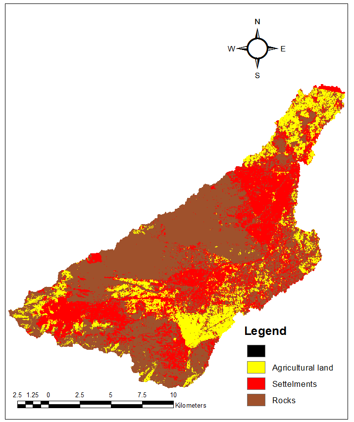
The total watershed of the Narai Canal was divided into three sub-watersheds (Figure 1). Discharge estimation of the sub-areas was included in the entire catchment area. Watershed 1 starts from the ring road and ends at the junction under Nasir Bagh Bridge Road. Watershed 2 starts from GT Road near Phase 3 Chowk, along with its upper region, and ends at the junction under Nasir Bagh Bridge Road. Watershed 3 starts from the junction under the Nasir Bagh Bridge Road to the bridge near Lalazar Colony, Peshawar, which is considered the outlet or control point for Watershed 3. The combined discharge at the last control point was recorded at the bridge near Lalazar Colony. After inputting data for the sub-areas and reaches, a data entry model was run to confirm that all data entries were correct and understood by the model.
The cross-section rating entry requires the input of ratings (elevation, discharge, end area, top width, and friction slope) for each stream routing reach. This information is developed outside of the Win-TR-20 software using uniform flow relationships, such as Manning’s Equation. The rainfall data, accounting for antecedent rainfall from average wet and dry years in the study area, were entered for rainfall type II to model storm analysis for the given return periods of 2, 5, 10, 25, 50, 100, and 200 years, respectively.
WinTR-20 (USDA-NRCS) was used to simulate rainfall–runoff processes and generate design hydrographs for the Narai watershed. The model was configured using watershed characteristics, channel geometry, and hydrological parameters derived from field measurements and GIS analysis. The watershed was represented as a single sub-watershed, and runoff was estimated using the NRCS Curve Number (CN) method. The CN value was derived from land use and hydrologic soil group maps under Antecedent Moisture Condition II (AMC-II), representing average soil moisture conditions recommended for design applications when antecedent rainfall information is unavailable (USDA-NRCS, 1986). The time of concentration (Tc) was estimated using the NRCS travel-time procedure, while the main channel length and average channel slope were extracted from the digital elevation model (DEM).
A 24-h NRCS Type II rainfall distribution was adopted to generate design storms because short-duration, high-intensity convective storms dominate the monsoon season in northwestern Pakistan, producing rainfall patterns comparable to the Type II distribution reported for semi-arid regions.
Model calibration was performed by adjusting the time of concentration (Tc) and Manning’s roughness coefficient (n) within physically realistic ranges to obtain agreement between the simulated and observed peak discharge at the Narai Canal. Because only a single observed runoff event was available, calibration was limited to matching the peak discharge, and no quantitative calibration performance metrics (e.g., RMSE, Nash–Sutcliffe efficiency, Kling–Gupta efficiency, or percent bias) were evaluated.
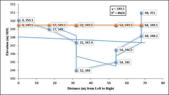
Channel routing was performed using the Muskingum routing method in WinTR-20. Field-surveyed channel cross-sections (Figure 2) were used to develop the stage–discharge relationship. Manning’s roughness coefficient was taken as 0.03, representing a natural earthen channel, while no constant baseflow was assigned because calibration was performed using individual storm events. A normal-depth outlet boundary condition based on the downstream channel slope was specified. Observed peak discharge used for calibration was estimated using the continuity equation:
\[Q = AV,\tag{13}\] \[V = \frac{1}{n}R^{2/3}S^{1/2},\tag{14}\] \[R = \frac{A}{P},\tag{15}\] \[S = \frac{\Delta H}{L},\tag{16}\] where Q is discharge (\(m^{3} s^{-1}\)), A is the flow cross-sectional area (\(m^{2}\)), V is flow velocity (\(m s^{-1}\)), n is Manning’s roughness coefficient, R is the hydraulic radius (m), P is the wetted perimeter (m), S is the hydraulic grade-line slope (\(mm^{-1}\)), \(\Delta H\) is the elevation difference, and L is the channel length. The measured channel cross-section used for discharge estimation is shown in Figure 2, while the hydraulic parameters are summarized in Table 1.
| Cross sectional area, A (\(m^{2}\)) | 55 |
| Wetted parameter, P (m) | 38.5 |
| Hydraulic radius, R (m) | 1.43 |
| Channel slope, S (m/m) | 0.01 |
| Manning’s roughness coefficient (n) | 0.03 |
| Flow velocity, V (m/s) | 14.5773 |
| Estimated discharge, Q (\(m^{3}/s\)) | 802 |
The Soil Conservation Service Curve Number (SCS-CN) method was used to estimate direct runoff from each sub-watershed. Curve numbers (CNs) were assigned by integrating land-use/land-cover (LULC) data with Hydrologic Soil Groups (HSGs) following the guidelines of the USDA Natural Resources Conservation Service (NRCS, TR-55). Each land-use/soil combination was assigned a standard CN value corresponding to Antecedent Moisture Condition II (AMC-II).
The weighted curve number for each sub-watershed was computed as the area-weighted average of all land-use/soil classes using \[CN_{w} = \frac{\sum\limits_{j=1}^{m}A_{j}CN_{j}}{\sum\limits_{j=1}^{m}A_{j}},\tag{17}\] where \(A_{j}\) is the area of land-use/soil class \(j\), \(CN_{j}\) is the corresponding curve number, and m is the total number of land-use/soil classes within the sub-watershed.
The resulting weighted curve numbers were subsequently used as input parameters in WinTR-20 runoff simulations together with the watershed area, time of concentration, rainfall depth, and rainfall distribution.
The rainfall–runoff relationship was evaluated by calculating the runoff coefficient (\(C_{r}\)), which represents the fraction of rainfall converted into direct runoff. The total runoff volume generated from the catchment was converted to an equivalent runoff depth by dividing it by the catchment area. The runoff coefficient was then calculated as the ratio of runoff depth to the corresponding rainfall depth:
\[C_{r} = \frac{Q_{d}}{P},\tag{18}\] where \(C_{r}\) is the runoff coefficient (dimensionless), \(Q_{d}\) is the runoff depth (mm), and P is the rainfall depth (mm).
The runoff coefficient was used solely to characterize the hydrological response of the catchment and to quantify the proportion of rainfall contributing to surface runoff. It was not interpreted as a measure of rainwater harvesting efficiency.
When the Win-TR-20 model successfully accepted all the relevant and appropriately formatted data, the model was calibrated against observed values to generate the required peak discharge and runoff volume. The calibrated model was then simulated to predict runoff for different return periods of 2, 5, 10, 25, 50, 100, and 200 years.
The WinTR-20 model is a rainfall–runoff simulation model, similar to HEC-HMS, that estimates watershed runoff using rainfall, land use, soil, and other catchment characteristics. Because continuous streamflow and discharge measurements are not available for the Narai Canal watershed, model calibration was performed using a reference peak discharge reported for the 2010 flood event rather than direct stream-gauging observations. A watershed-average rainfall depth of 233 mm was used as the model input, which generated a previously reported (reconstructed) peak discharge of 802 \(m^{3} s^{-1}\) at the watershed outlet. In contrast, the 294 mm value represents the maximum 24-h rainfall recorded at a single station during the same event. The 2010 storm was subsequently evaluated against the LP-III frequency analysis to compare its magnitude with rainfall depths associated with different return periods. The model parameters, particularly the time of concentration (\(Tc\)) and Manning’s roughness coefficient (\(n\)), were iteratively adjusted until the simulated peak discharge closely matched the reported reference value. The outlet cross-sectional geometry was assumed to remain unchanged during the calibration process. After calibration, the model was driven with design rainfall depths corresponding to the 2, 5, 10, 25, 50, 100, and 200 year return periods to estimate peak runoff and generate design hydrographs for the Narai Canal watershed.
The rainfall frequency analysis was conducted under the assumption of stationarity, whereby the statistical characteristics of the annual maximum rainfall series were considered unchanged throughout the observation period. Consequently, the estimated design rainfall and corresponding runoff simulated using WinTR-20 reflect historical climatic conditions. Although this assumption is commonly adopted in engineering hydrology, future changes in rainfall extremes associated with climate variability may influence the reliability of design estimates. Therefore, the results should be interpreted as baseline design values, and future studies should evaluate rainfall non-stationarity using statistical trend and change-point analyses or non-stationary frequency models to improve the robustness of hydraulic design.
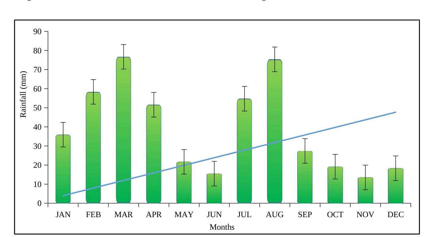
Daily maximum precipitation data for each month over the past four decades in Peshawar was acquired from the Pakistan Meteorological Department (PMD). Analysis of the data indicated that March and August exhibited the highest average rainfall, with 76.7 mm and 75.4 mm respectively (Figure 3). Conversely, June and November were identified as the months with the lowest average rainfall, recording 15.5 mm and 13.5 mm respectively. These findings offer valuable insights into the rainfall patterns of Peshawar over the studied period, aiding in better understanding and management of water resources and infrastructure in the region.
The results of the study emphasize the use of Easy Fit software to fit frequency distributions, applying the Chi-Square test to identify the most appropriate model for estimating rainfall amounts across different return periods. The return periods, ranging from 2 to 200 years, are associated with their respective rainfall amounts in millimeters. The findings indicated that rainfall estimates increased with longer return periods, highlighting their importance in predicting and preparing for extreme weather events. The Log-Pearson Type III distribution was identified as the best fit based on the analysis conducted through Easy Fit software (Table 2).
| S. No. | Return Period (years) | Rainfall (mm) |
|---|---|---|
| 1 | 2 | 56 |
| 2 | 5 | 83 |
| 3 | 10 | 106 |
| 4 | 25 | 142 |
| 5 | 50 | 175 |
| 6 | 100 | 213 |
| 7 | 200 | 258 |
The annual maximum one-day rainfall series (1985–2025) was used for frequency analysis. The dataset comprised 41 annual observations (N = 41), as presented in Table 1. Following the recommendations of the U.S. Water Resources Council Bulletin 15 [31], the annual maximum rainfall values were transformed using the common logarithm (base-10) prior to fitting the LP-III distribution. The sample mean of the logarithms, sample standard deviation, and sample skewness coefficient were calculated from the transformed series and used to estimate the LP-III distribution parameters by the method of moments.
The suitability of the LP-III distribution was evaluated in EasyFit by comparing it with several commonly used probability distributions, including the Normal, Lognormal, Gamma, Weibull, Gumbel, Pearson Type III, and Generalized Extreme Value (GEV) distributions. Candidate distributions were ranked using the chi-square goodness-of-fit test based on the fitted distributions. Among the evaluated models, the LP-III distribution produced the lowest chi-square statistic and was therefore selected for rainfall frequency analysis. The fitted LP-III parameters obtained from EasyFit were shape (\(\alpha\)) = 17.559, scale (\(\beta\)) = \(-0.14425\), and location (\(\gamma\)) = 6.8339.
| Parameters | Values | ||||
|---|---|---|---|---|---|
| Deg. of freedom | 4 | ||||
| Statistics | 0.22267 | ||||
| P- Value | 0.99424 | ||||
| Rank | 1 | ||||
| \(\alpha\) (Significance level) | 0.2 | 0.1 | 0.05 | 0.02 | 0.01 |
| Critical Value | 5.9886 | 7.7794 | 9.4877 | 11.668 | 13.277 |
| Reject? | No | No | No | No | No |
The chi-square goodness-of-fit statistics are presented in Table 3. The calculated chi-square statistic was 0.22267 with 4 degrees of freedom and a corresponding p-value of 0.99424. Since the calculated statistic was lower than the critical values at all tested significance levels (0.20–0.01), the null hypothesis was not rejected, indicating that the observed rainfall series is adequately represented by the LP-III distribution.
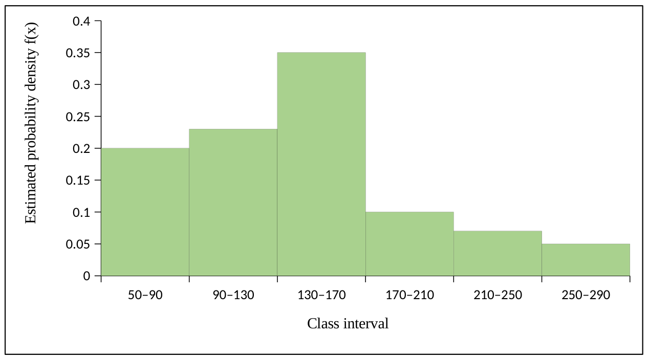
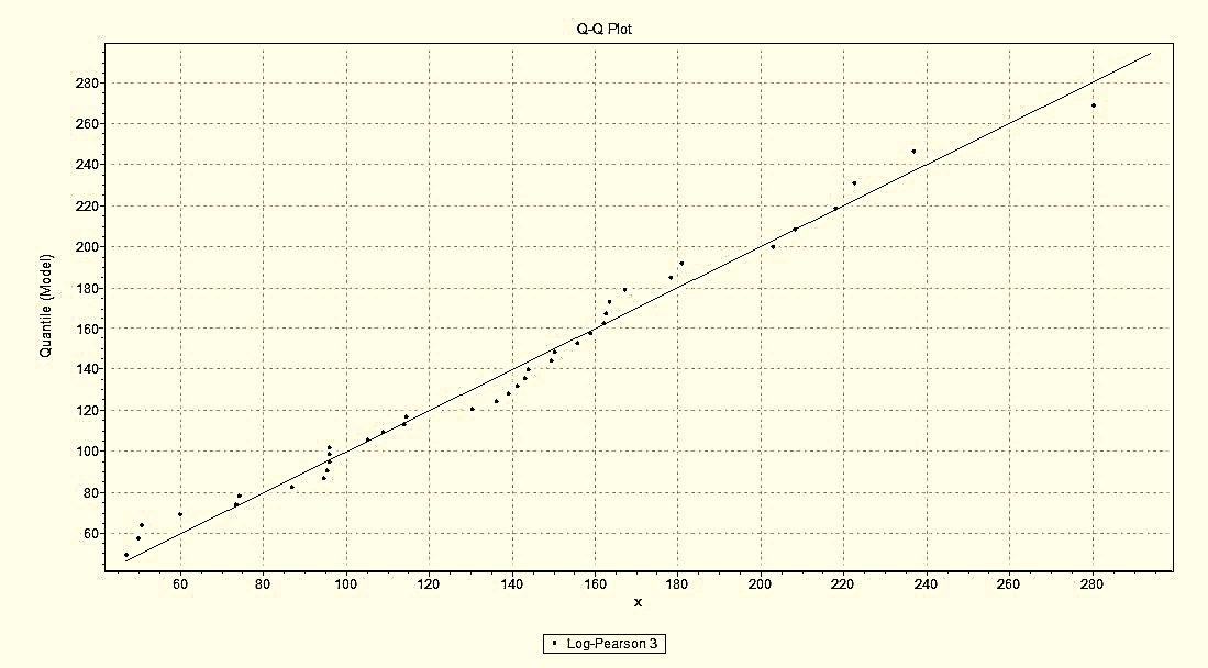
The frequency histogram (Figure 4) shows that the fitted LP-III distribution closely follows the observed rainfall–runoff frequency distribution, indicating good agreement between the empirical and theoretical distributions. Similarly, the quantile–quantile (Q–Q) plot (Figure 5) demonstrates that the observed and theoretical quantiles closely align along the 1:1 reference line, with only minor deviations at the distribution tails, confirming the adequacy of the fitted model over the observed data range.
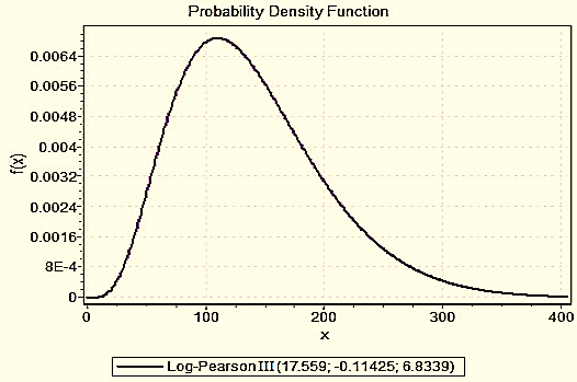
The Probability Distribution Function (PDF) for the Log-Pearson Type III distribution illustrates the probability of different outcomes by providing a graphical view of how rainfall-runoff values are distributed. The PDF highlights regions of higher probability, where values are more likely to occur, as well as areas of lower probability, where outcomes are less frequent. This visualization is particularly important in hydrological studies, as it allows for a clearer understanding of the variability and extremes of rainfall-runoff events. By examining the curve, one can identify patterns such as skewness, central tendency, and the spread of data, which are critical for assessing flood risks, planning water resource management, and developing mitigation strategies. The use of the Log-Pearson Type III distribution in this context ensures a more accurate representation of extreme hydrological events, making it a valuable tool for both researchers and practitioners in the field of water management (Figure 6).
The results of the study estimated the maximum rate of water runoff during a particular storm event from various watersheds. This prediction is essential for understanding and managing water resources, especially in the context of flood forecasting and mitigation. To make these predictions, several parameters are considered, including the area of the watershed, land use characteristics, rated curve numbers (RCN), and time of concentration (Tc) (Figure 7). The runoff rate in cubic meters per second (\(m^{3}/s\)) was estimated based on these parameters.
The areas of different land use within each watershed are presented in Table 4. The findings of the study list the identification of each watershed along with its total area, agricultural land area, settlement area, and area covered by rocks. For example, Watershed 1 has a total area of 178.5 \(km^{2}\), with 28.5 \(km^{2}\) designated for agricultural land, 57.2 \(km^{2}\) for settlements, and 92.9 \(km^{2}\) for rocks.
| Watershed Identification | Area (\(km^{2}\)) | Agricultural Land (\(Km^{2}\)) | Settlement (\(Km^{2}\)) | Rocks (\(Km^{2}\)) |
|---|---|---|---|---|
| Watershed 1 | 178.5 | 28.5 | 57.2 | 92.9 |
| Watershed 2 | 58.2 | 2.5 | 20 | 35.7 |
| Watershed 3 | 18.4 | 9.5 | 4.4 | 4.5 |
The weighted Curve Numbers (CNs) were derived by combining land-use classes with their corresponding hydrologic soil groups using the NRCS Curve Number method. Class-specific CN values were assigned from the NRCS National Engineering Handbook and weighted according to the proportional area occupied by each land-use class within individual sub-watersheds.
The land-use composition, assigned Curve Numbers, and weighted CN values for the three sub-watersheds is shown in Table 5. Agricultural land constituted the dominant land-use category, followed by rangeland and exposed rock. Rock outcrops were assigned a CN of 98 because of their negligible infiltration capacity and high runoff potential. The computed weighted CN values were 80.28, 75.50, and 70.50 for Sub-watersheds 1, 2, and 3, respectively (Table 6). These values indicate a gradual decrease in runoff potential from the upstream to downstream sub-watersheds, primarily due to variations in land cover and infiltration characteristics.
| Sub-watershed | Land-use class | Hydrologic soil group | Assigned CN* | Area (\(km^{2}\)) | Weighted CN Contribution |
|---|---|---|---|---|---|
| SW-1 | Agric. land | C | 82 | 95.20 | 43.74 |
| SW-1 | Rangeland | C | 74 | 36.10 | 14.97 |
| SW-1 | Built-up area | C | 90 | 15.60 | 7.87 |
| SW-1 | Exposed rock | Impervious | 98 | 31.58 | 17.34 |
| SW-1 | Total | — | — | 178.48 | 80.28 |
| SW-2 | Agric. land | B | 78 | 28.30 | 37.95 |
| SW-2 | Rangeland | B | 69 | 13.20 | 15.65 |
| SW-2 | Built-up area | C | 90 | 5.20 | 8.05 |
| SW-2 | Exposed rock | Impervious | 98 | 11.47 | 13.85 |
| SW-2 | Total | — | — | 58.17 | 75.50 |
| SW-3 | Agric. land | B | 75 | 10.15 | 41.39 |
| SW-3 | Rangeland | B | 69 | 4.05 | 15.19 |
| SW-3 | Built-up area | B | 85 | 1.12 | 5.18 |
| SW-3 | Exposed rock | Impervious | 98 | 3.07 | 8.74 |
| SW-3 | Total | — | — | 18.39 | 70.50 |
| Sub-watershed | Area (\(Km^{2}\)) | Reach | Weighted Curve Number (CNw) | Time of Concentration Tc (hr) |
|---|---|---|---|---|
| SW-1 | 178.48 | R-1 | 80.28 | 11 |
| SW-2 | 57.17 | R-2 | 75.50 | 10.18 |
| SW-3 | 18.39 | Outlet | 70.50 | 10.28 |
The weighted CNs, together with watershed area and time of concentration, served as primary inputs for the WinTR-20 rainfall–runoff simulations. Higher weighted CN values corresponded to greater runoff generation and consequently higher simulated peak discharges during design storm events.
The estimated time of concentration ranged from 10 to 11 h among the sub-watersheds. These values reflect the relatively long hydraulic flow paths and low average watershed slopes derived from the DEM, resulting in a moderate runoff response. The computed \(T_{c}\) values were subsequently used in WinTR-20 to generate runoff hydrographs and estimate peak discharges for the design storm events.
The stream reach and receiving identifiers, along with their respective cross sections and lengths, are provided in Table 7. The results point out the identifiers for the stream reaches, their corresponding receiving reaches, the cross-section rating names, and both the channel and valley lengths in meters. Specifically, Reach R-1 connects to Reach R-3 with a cross-section rating of CR-1, having both a channel and valley length of 20,584 meters. Reach R-2 also connects to Reach R-3, with a cross-section rating of CR-2, and both a channel and valley length of 10,363 meters. Finally, Reach R-3 flows into the Outlet with a cross-section rating of CR-3, having both a channel and valley length of 2,050 meters.
| Canal reach identifier | Canal receiving reach identifier | Canal cross section rating name | Reach channel length (m) | Reach valley length (m) |
|---|---|---|---|---|
| R-1 | R-3 | CR-1 | 20584 | 20584 |
| R-2 | R-3 | CR-2 | 10363 | 10363 |
| R-3 | Outlet | CR-3 | 2050 | 2050 |
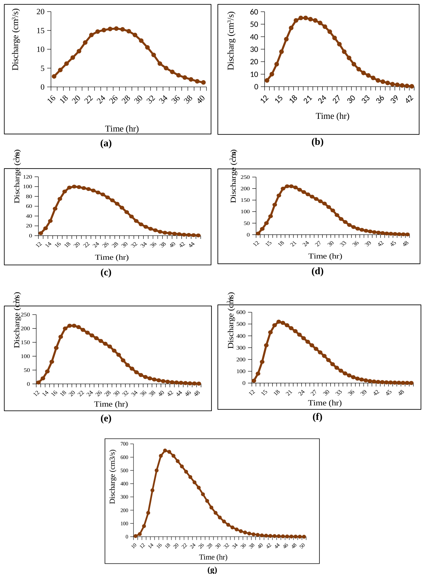
The peak runoff rate, time duration, and elevation are presented in Table 8. Hydrographs for return periods of 2, 5, 10, 25, 50, 100, and 200 years were predicted using the Win-TR-20 model, as shown in Figure 8 (a, b, c, d, e, f, g). These hydrographs for the Narai Canal watershed have been delineated at the Lalazar Bridge (outlet) using the Win-TR-20 model, incorporating information about land use, topography, and rainfall.
| Return periods (years) | 2 | 5 | 10 | 25 | 50 | 100 | 200 |
|---|---|---|---|---|---|---|---|
| Rainfall (mm) | 56 | 83 | 106 | 142 | 175 | 213 | 258 |
| Runoff (mm) | 3.02 | 12.08 | 23.81 | 44.34 | 66.85 | 95.27 | 131.31 |
| Peak Discharge (\(m^{3}/s\)) | 15.6 | 54.7 | 104 | 208 | 319 | 462.5 | 649.8 |
| Elevation (m) | 344.56 | 344.96 | 345.28 | 345.71 | 346.05 | 346.41 | 346.81 |
| Time Duration (hr) | 15.6 | 22.74 | 20.81 | 19.29 | 19.51 | 18.88 | 18.71 |
Detailed information on the peak discharges and elevations at the outlet for different return periods, ranging from 2 to 200 years is shown in Figure 8. The results include data on rainfall amounts, runoff volumes, peak discharge rates, elevations, and time durations for each return period. For instance, the peak discharge increases from 15.6 \(m^{3}/s\) for a 2-year return period to 649.8 \(m^{3}/s\) for a 200-year return period, indicating the significant variation in runoff and discharge with increasing rainfall intensity. Elevation levels at the outlet also show a gradual rise with higher return periods, reflecting the impact of larger runoff volumes on the water surface elevation. The time duration for peak discharge varies slightly across the different return periods, indicating how quickly the peak flow is reached during different storm events.
The Rainfall-Runoff relationship for different return periods ranging from 2 to 200 years has already been discussed under various hydrographs. Table 9 presents the Runoff Coefficients derived from this relationship, indicating that only 5% of the rain can be harvested from a rainfall of 50 mm in the watershed over a return period of 2 years.
| Return periods (years) | 2 | 5 | 10 | 25 | 50 | 100 | 200 |
|---|---|---|---|---|---|---|---|
| Rainfall (mm) | 56 | 83 | 106 | 142 | 175 | 213 | 258 |
| Runoff (mm) | 3.02 | 12.08 | 23.81 | 44.34 | 66.85 | 95.27 | 131.31 |
| Runoff Coefficient | 0.05 | 0.15 | 0.22 | 0.31 | 0.38 | 0.45 | 0.51 |
| Differences | – | 0.09 | 0.08 | 0.09 | 0.07 | 0.07 | 0.06 |
| Differences in (%) | – | 9 | 8 | 9 | 7 | 7 | 6 |
From a storm of 83 mm in a five-year return period, the runoff improves to 15% (three times more than the 2-year return period), which increases to 22% for a 10-year return period. The runoff coefficient improves to 31% for a 25-year return period. The trend of increasing runoff coefficient is observed between the 2- and 5-year, 5- and 10-year, and up to 25-year return periods. Similarly, there is an increase in efficiency between the 25- and 50-year, 50- and 100-year, and 100- and 200-year return periods, with nearly a 7% increase in each case. Overall, the runoff coefficient for a 200-year return period is ten times greater than that of a 2-year return period.
Similarly, the findings of the study revealed that with the increase of return period from 2 to 200 years, both the rainfall and the corresponding runoff increase. The runoff coefficients, which represent the fraction of rainfall that becomes runoff, also increase with longer return periods. The differences and percentage differences in runoff coefficients highlight the incremental changes between successive return periods. This information is important for understanding the efficiency of rainwater harvesting and the hydrological response of the watershed over different time scales.
Rainfall-runoff relationships were developed to analyze the correlation between rainfall (mm) and runoff depth (mm). The analysis involves plotting rainfall events against the corresponding runoff depths to understand how varying rainfall intensities affect runoff generation within the watershed (Figure 9). This relationship provides valuable information for predicting runoff volumes based on expected rainfall, which can inform flood management and water resource planning. By studying the patterns in the data, it becomes evident how efficiently rainfall is converted to runoff, which is influenced by factors such as soil saturation, land cover, and topography.
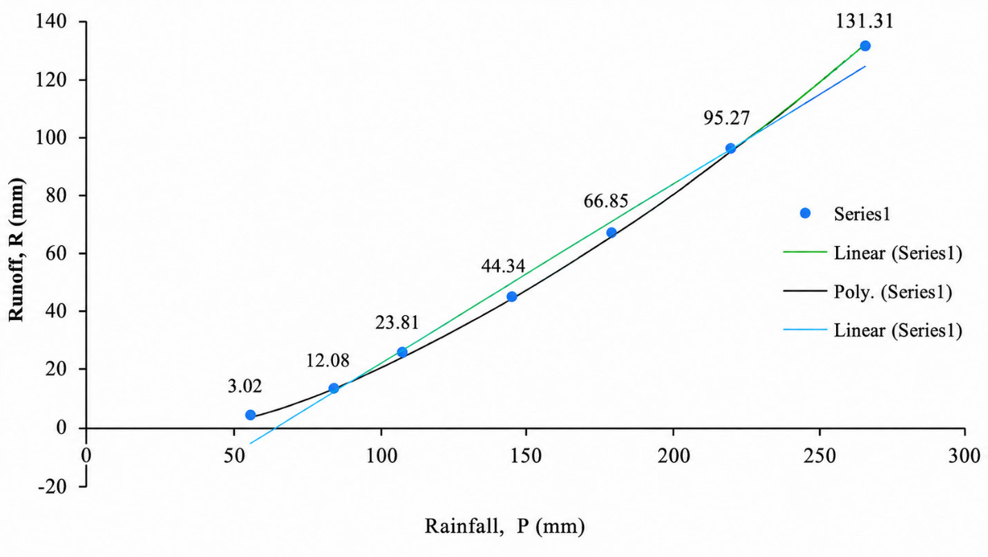
A comprehensive understanding of rainfall-runoff processes is crucial for watersheds with variable streamflow generation, as proper knowledge of runoff is essential for planning and designing water resources and related projects [32]. Estimating runoff volume and peaks is also vital for planning various interventions in integrated watershed management and flood protection projects [33]. However, detailed hydrological studies face challenges due to data scarcity and the complexity of hydrological systems. The runoff simulation model is a hydrological tool that can simulate watershed rainfall responses and forecast floods for water resources management [34]. Flood simulation is facilitated by employing a model and understanding the factors that trigger runoff [35]. Different models, however, require numerous input parameters that are not easily obtainable [36]. Therefore, it is necessary to select a model with a simple structure, minimal input data, and accurate predictions [37]. This study aimed to assess the rainfall-runoff relationship for the Narai Canal using the Log Pearson Type III Distribution and Win TR-20 model, yielding significant insights into the hydrological dynamics of the region. The results demonstrate the applicability and accuracy of these models in predicting peak runoff rates, which is vital for flood management and mitigation efforts.
The Log Pearson Type III Distribution has been widely acknowledged for its effectiveness in hydrological frequency analysis, particularly in estimating extreme events [38]. Our findings align with recent studies that highlight the reliability of distribution in handling diverse hydrological datasets and its robustness in predicting return periods for various storm events [39]. The Win TR-20 model proved instrumental in simulating the hydrological response of the watershed. This ability of the model to incorporate diverse land use and hydrological parameters, such as rated curve numbers and time of concentration, allowed for a detailed analysis of runoff generation and peak discharge [40]. The study results indicated that urbanization and land use changes significantly impact runoff rates, a finding corroborated by recent studies emphasizing the need for integrated land and water management in urban watersheds [41,42].
One of the important aspects highlighted by the findings of the study is the importance of accurate rainfall data in hydrological modeling [43]. Rainfall is the primary input for many design calculations, and the accuracy of the modeling results is highly dependent on the consistency and resolution of the rainfall monitoring network. The paper emphasizes that long historical rainfall series should be used for modeling, and a statistical analysis should be performed on the results to ensure the reliability of the findings. The results also address the challenges associated with hydrologic modeling, particularly the ease of producing similar hydrographs, which can lead to problems in parameter fitting and the criteria used for measuring accuracy. The fitting of parameters and the selection of appropriate criteria for evaluating model performance are two major problems in hydrologic modeling, as highlighted in previous research studies [44,45].
Our results indicated that runoff coefficient continues to improve across various return periods: from two to five years, five to ten years, and up to 25 years. similarly, a steady increase in efficiency was observed between the 25- and 50-year, 50- and 100-year, and 100- and 200-year return periods, with each interval showing an approximate 7% rise. These observations align with Vangelis et al. [46], who noted that a 25-year return period and a 50-year flood event correspond to rainfall with a return period of roughly 110 years. The observed variations in peak runoff rates across different return periods underscore the importance of historical rainfall data in hydrological modeling. Our use of rainfall data spanning four decades (1985-2025) provided a comprehensive overview of temporal changes in rainfall patterns and their impact on runoff. Similar long-term studies have demonstrated the critical role of extensive historical data in enhancing the accuracy of hydrological models [47]. Thus, the design of hydraulic structures in the study area requires consideration of larger return periods of rainfall.
The practical implications of the findings of the proposed study are significant for flood forecasting and mitigation in Peshawar. The accurate prediction of peak runoff rates can inform the design and implementation of effective flood control measures, reducing the risk of flood-related damages. This study highlighted the necessity of continuous monitoring and updating of hydrological models to account for ongoing changes in land use and climate conditions [48], emphasizing the importance of integrating advanced hydrological models with extensive historical data to improve flood forecasting and water resource management. Future research should focus on incorporating real-time data and exploring the impacts of climate change on runoff patterns to further enhance the predictive capabilities of these models.
This study developed a design-storm rainfall–runoff analysis for the Narai Canal catchment using the LP-III distribution and the WinTR-20 model under ungauged-basin conditions. Design rainfall corresponding to different return periods was estimated using the LP-III distribution, while runoff hydrographs and peak discharges were simulated using the SCS curve number method within the WinTR-20 framework. The results showed that runoff magnitude and peak discharge increased with rainfall intensity and return period, highlighting the importance of watershed characteristics, including land use, curve number, and time of concentration, in runoff generation. Because no observed discharge data were available, the model could not be calibrated or independently validated. Consequently, the findings were interpreted as a preliminary hydrological assessment and design-scenario analysis, rather than as a validated rainfall–runoff or operational flood-forecasting model. Nevertheless, the generated design hydrographs and peak discharge estimates provide useful information for preliminary canal hydraulic design, drainage planning, and flood-risk assessment in data-scarce catchments.
Future research should focus on establishing streamflow monitoring stations, collecting observed discharge data for model calibration and independent validation, and evaluating additional hydrological models to improve predictive accuracy. These improvements would support the future development of reliable operational flood-forecasting and water resources management systems for the Narai Canal watershed.
This study contributes a site-specific hydrological assessment of the Narai Canal catchment in Peshawar, Pakistan, through the integrated application of Log-Pearson Type III frequency analysis, the SCS Curve Number method, and WinTR-20 runoff simulation. Rather than introducing a new modeling framework, its originality lies in providing the first comprehensive application of this established workflow to support rainfall–runoff characterization and design discharge estimation for the Narai Canal system. The results provide locally relevant hydrological information that improves understanding of runoff response in this semi-arid canal catchment and offers a practical basis for canal design, flood risk assessment, and water resources planning. These findings also provide a useful reference for hydrological studies and infrastructure management in similar canal systems across Peshawar and other semi-arid regions.
Acknowledgments: The author is thankful to the Partnership for Applied Sciences, Engineering, and Technology (PASET) – Regional Scholarship and Innovation Fund (RSIF) for the support of this study.
Conflicts of Interest: The authors declare that there is no conflict of interest whatsoever with any affiliation, or involvement with any organization, financial and non-financial entity.