
The domination number \(\gamma(G)\) is the minimum cardinality of a set \(D\subseteq V(G)\) such that every vertex of \(G\) lies in \(D\) or has a neighbor in \(D\). Such a set is called a dominating set, and it is called a \(\gamma\)-set when \(|D|=\gamma(G)\). The dominion \(\zeta(G)\) is the number of \(\gamma\)-sets of \(G\).
Introduced by Allagan and Bobga [1], \(\zeta(G)\) distinguishes graphs with the same domination number but different numbers of optimal configurations, a distinction not detected by \(\gamma\) alone. In network design and control, vertices may represent facilities, sensors, or agents that monitor a system, and \(\zeta(G)\) measures the availability of alternative optimal configurations under node failures or forced reconfiguration [2]. This perspective appears in wireless sensor networks [3–5], Internet of Things architectures [6,7], distributed computing [8], network security [9,10], facility location [11,12], influence maximization [13], and epidemic control [14].
The enumeration of minimum dominating sets has developed along several directions. Exact counts for paths, cycles, and grids appear in [1,15]. Godbole, Jamieson, and Jamieson [16] and Connolly et al. [17] established exponential upper bounds on \(\zeta\) in terms of \(\gamma\), while Goddard and Henning [18] characterized graphs with a unique \(\gamma\)-set. The sharpest forest bound is due to Petr, Portier, and Versteegen [19], who proved \(\zeta(F)\le 5^{\gamma(F)}\) and constructed families of order \(5^{2\gamma(F)/5}\), establishing the correct exponential rate up to constant factors.
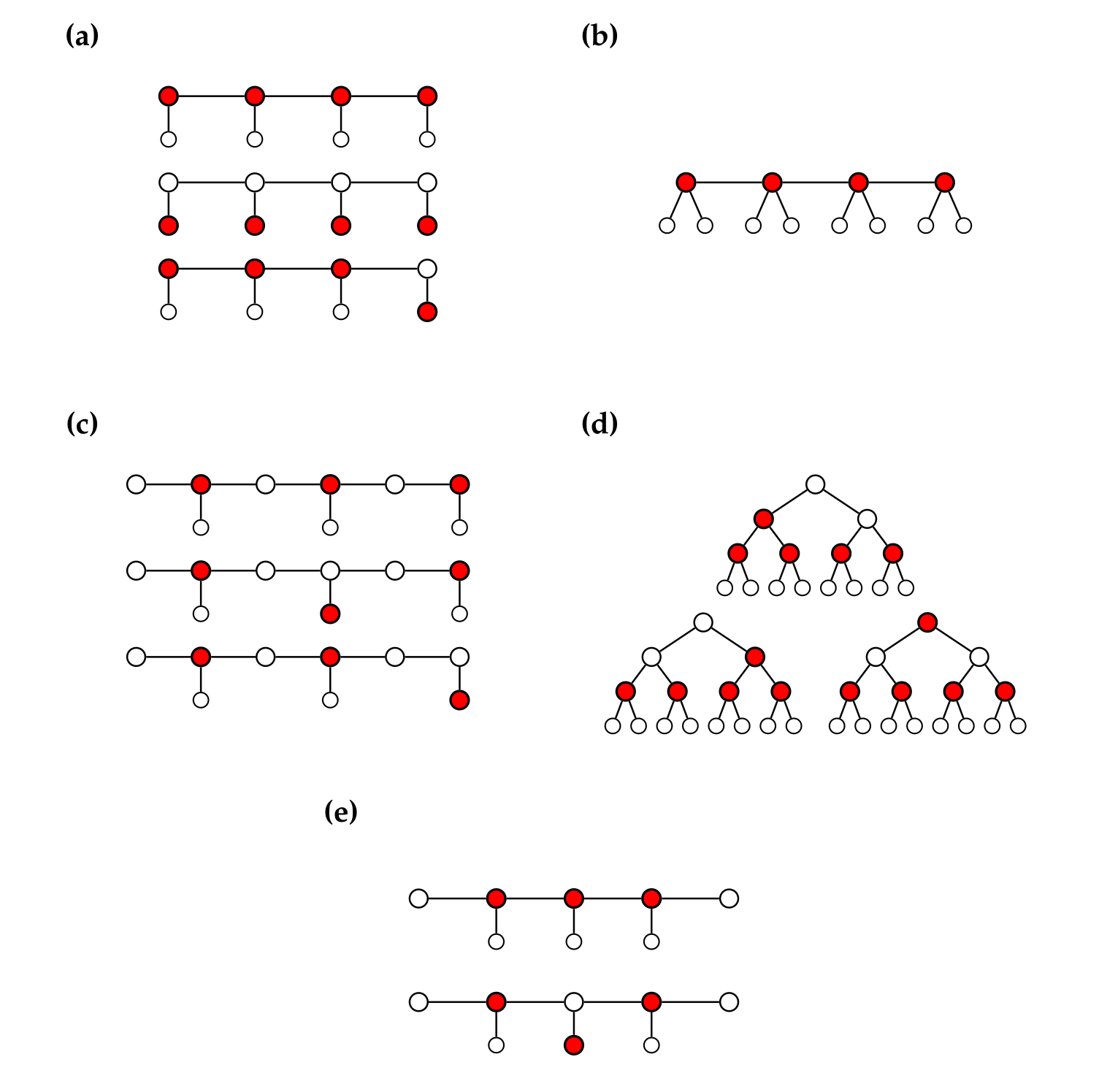
We take a complementary structural approach. Rather than extremizing \(\zeta\) over all trees with fixed \(\gamma\), we compute \(\gamma\) and \(\zeta\) exactly for canonical tree families and identify the local mechanisms that determine the number of optimal configurations. Four behaviors arise: (i) exponential freedom, where independent pendant clusters give \(\zeta=2^{\gamma}\); (ii) Fibonacci growth, where nearest-neighbor coupling gives \(\zeta\asymp\varphi^{\gamma}\); (iii) periodic rigidity, where complete binary trees satisfy \(\zeta(T_h)\in\{1,3\}\) despite exponential growth of \(|V(T_h)|\); and (iv) complete forcing, where high pendant density gives \(\zeta=1\). Figure 1 illustrates these forms of optimal domination.
We also analyze the stability of complete binary trees under leaf deletion. Deleting a single leaf of \(T_h\) preserves \(\gamma\) and exactly doubles \(\zeta\). More generally, if \(X\subseteq L_h\) is sparse in the sense that no parent in \(L_{h-1}\) loses both of its leaf children, then \(\zeta(T_h-X)\le 2^{m_1(X)}\zeta(T_h)\), where \(m_1(X)\) is the number of parents in \(L_{h-1}\) that lose exactly one child. These results show that the rigidity of complete binary trees is locally fragile while the families studied here remain well below the general forest envelope \(\zeta(F)\le 5^{\gamma(F)}\) of [19].
Throughout, \(P_n\) denotes the path \(v_1v_2\cdots v_n\). For \(n\ge 1\) and \(r\ge 1\), let \(L_i=\{\ell_{i,1},\dots,\ell_{i,r}\}\) be the set of \(r\) pendant vertices attached to \(v_i\); the graph \(G(n,r)\) denotes \(P_n\) with this uniform attachment, and \(G_n=G(n,1)\) is the \(n\)-comb. The complete binary tree of height \(h\) is denoted \(T_h\), with \(|V(T_h)|=2^{h+1}-1\). The Fibonacci sequence \((F_t)_{t\ge 1}\) is defined by \(F_1=F_2=1\) and \(F_{t+1}=F_t+F_{t-1}\).
Domination in each family below is controlled by local clusters, each consisting of a path vertex and its attached pendants. Whether the \(\gamma\)-sets of the whole graph are unique, fully independent across clusters, or constrained by a Fibonacci recurrence depends entirely on the attachment pattern, and the three families together realize dominion growth with bases \(1\), \(\varphi\), and \(2\).
Theorem 1 (Forcing dichotomy). Fix integers \(n\ge 1\) and \(r\ge 1\), and let \(G(n,r)\) be the graph obtained from \(P_n\) by attaching \(r\) pendant vertices \(\ell_{i,1},\dots,\ell_{i,r}\) to each \(v_i\). Then \(\gamma(G(n,r))=n\) and \[\zeta(G(n,r))= \begin{cases} 2^n, & r=1,\\ 1, & r\ge 2. \end{cases}\]
When \(r\ge 2\) the unique \(\gamma\)-set is \(\{v_1,\dots,v_n\}\); when \(r=1\) every \(\gamma\)-set arises from an independent choice of one vertex from each pair \(\{v_i,\ell_{i,1}\}\).
Proof. For each \(i\), the closed neighborhood of any pendant \(\ell\in L_i\) is \(N[\ell]=\{\ell,v_i\}\), so every dominating set must meet the cluster \(\{v_i\}\cup L_i\). The \(n\) clusters are pairwise disjoint, hence \(\gamma(G(n,r))\ge n\), and \(\{v_1,\dots,v_n\}\) witnesses equality.
Let \(D\) be a \(\gamma\)-set, so \(|D|=n\). Disjointness forces \(|D\cap(\{v_i\}\cup L_i)|=1\) for every \(i\). If \(r\ge 2\) and \(v_i\notin D\), then every pendant in \(L_i\) must dominate itself, forcing \(L_i\subseteq D\) and contradicting \(|D\cap(\{v_i\}\cup L_i)|=1\); hence \(v_i\in D\) for all \(i\), giving \(\zeta(G(n,r))=1\). If \(r=1\), exactly one vertex from \(\{v_i,\ell_{i,1}\}\) belongs to \(D\) at each position, and any such choice dominates the pair; the \(n\) choices are independent, yielding \(\zeta(G(n,1))=2^n\). \(\square\)
The star \(K_{1,m}\) is the special case \(G(1,m)\), so \(\gamma(K_{1,m})=1\) and \(\zeta(K_{1,m})=2\) when \(m=1\), and \(\zeta(K_{1,m})=1\) when \(m\ge 2\). Likewise, the \(n\)-comb is \(G_n=G(n,1)\), and Theorem 1 gives \(\gamma(G_n)=n\) and \(\zeta(G_n)=2^n=2^{\gamma(G_n)}\). Figure 1(a) shows three of the \(2^4=16\) minimum dominating sets of \(G_4\), while Figure 1(b) shows the unique \(\gamma\)-set of \(G(4,2)\).
If the two endpoints \(v_1\) and \(v_n\) carry no pendant, each must be dominated by its unique path neighbor, forcing \(v_2\) and \(v_{n-1}\) into every \(\gamma\)-set and reducing \(\zeta(G’_n)\) by a factor of \(4\) relative to the full comb. The case when \(n=5\) is shown in Figure 1(e).
Theorem 2 (Interior pendants). Let \(G’_n\) be obtained from \(P_n\) by attaching one pendant \(\ell_i\) to each internal vertex \(v_i\) for \(2\le i\le n-1\). Then \(\gamma(G’_n)=\max\{1,n-2\}\) and \[\zeta(G’_n)= \begin{cases} 2, & n=2,\\ 1, & n=3,\\ 2^{\gamma(G’_n)-2}, & n\ge 4. \end{cases}\]
Proof. For \(2\le i\le n-1\) set \(C_i=\{v_i,\ell_i\}\). Since \(N[\ell_i]=C_i\), every dominating set meets each \(C_i\), giving \(|D|\ge n-2\) for \(n\ge 3\). As \(\{v_2,\dots,v_{n-1}\}\) dominates \(G’_n\), \(\gamma(G’_n)=\max\{1,n-2\}\). The cases \(n=2\) and \(n=3\) follow by inspection.
Let \(n\ge 4\) and suppose \(D\) is a \(\gamma\)-set, so \(|D|=n-2\). Cluster forcing gives \(|D\cap C_i|=1\) for each \(2\le i\le n-1\). If \(\ell_2\in D\), then \(v_1\) has no neighbor in \(D\) and is undominated, contradicting \(|D|=n-2\); hence \(v_2\in D\). The identical argument at \(v_n\) forces \(v_{n-1}\in D\). Every \(\gamma\)-set therefore takes the form \[D=\{v_2,v_{n-1}\}\cup\{x_i:3\le i\le n-2\},\qquad x_i\in\{v_i,\ell_i\}.\]
For \(n\ge 5\), the vertex \(v_2\) covers \(\{v_1,v_2,v_3,\ell_2\}\) and \(v_{n-1}\) covers \(\{v_{n-2},v_{n-1},v_n,\ell_{n-1}\}\), so the \(n-4\) choices of \(x_i\) are independent and each dominates \(C_i\). For \(n=4\) the set \(\{v_2,v_3\}\) is the unique \(\gamma\)-set, consistent with \(2^0=1\). In both cases \(\zeta(G’_n)=2^{n-4}=2^{\gamma(G’_n)-2}\). \(\square\)
When pendants are attached only to alternating vertices of \(P_n\), each path vertex carrying no pendant lies between two clusters and must be dominated by one of its two path neighbors. This constraint couples adjacent cluster choices and gives rise to a Fibonacci recurrence in place of full independence.
For \(n\ge 2\), let \(E_n\) (resp. \(O_n\)) be the graph obtained from \(P_n\) by attaching one pendant \(\ell_i\) to each even-indexed (resp. odd-indexed) vertex \(v_i\).
Theorem 3 (Fibonacci dominion for alternating combs). Let \(n\ge 2\) and set \(k=\lfloor n/2\rfloor\). Then \[\gamma(E_n)=k,\qquad \zeta(E_n)= \begin{cases} F_{k+1},& n=2k,\\ F_k,& n=2k+1, \end{cases}\] and \[\gamma(O_n)=\lceil n/2\rceil,\qquad \zeta(O_n)= \begin{cases} F_{k+1},& n=2k,\\ F_{k+3},& n=2k+1, \end{cases}\] where \((F_t)_{t\ge1}\) denotes the Fibonacci sequence defined by \(F_1=F_2=1\) and \(F_{t+1}=F_t+F_{t-1}\).
Proof. We begin with the even attachment family. For each even index \(2i\), the pair \(C_{2i}=\{v_{2i},\ell_{2i}\}\) forms a pendant cluster satisfying \(N[\ell_{2i}]=C_{2i}\). Since no vertex outside \(C_{2i}\) dominates \(\ell_{2i}\), every dominating set must intersect each such cluster. As these \(k\) clusters are pairwise disjoint, it follows that \(\gamma(E_n)\ge k\). The set \(\{v_2,v_4,\dots,v_{2k}\}\) dominates \(E_n\), establishing \(\gamma(E_n)=k\).
To enumerate minimum dominating sets, consider the graph \(H_t\) obtained from \(E_{2t}\) by restricting to vertices \(v_1,\dots,v_{2t}\) together with pendants \(\ell_2,\ell_4,\dots,\ell_{2t}\), and define \(a_t=\zeta(H_t)\). Every minimum dominating set selects exactly one vertex from each cluster, so \(|D|=t\). Direct inspection gives \(a_1=1\) and \(a_2=2\). For \(t\ge 3\), let \(D\) be a minimum dominating set and examine the final cluster \(C_{2t}\). If \(v_{2t}\in D\), then removing \(\{v_{2t-1},v_{2t},\ell_{2t}\}\) yields a minimum dominating set of \(H_{t-1}\). If instead \(\ell_{2t}\in D\), then \(v_{2t}\notin D\) and the vertex \(v_{2t-1}\) must be dominated by \(v_{2t-2}\), which is therefore forced into \(D\); removing the vertices \(\{v_{2t-3},v_{2t-2},v_{2t-1},v_{2t},\ell_{2t}\}\) leaves a subgraph isomorphic to \(H_{t-2}\). The two constructions are disjoint because the terminal cluster \(C_{2t}\) is represented by either \(v_{2t}\) or \(\ell_{2t}\), never both; they are exhaustive because every minimum dominating set realizes exactly one of these two possibilities; and each reduction is reversible by reattaching the removed vertices and restoring the unique forced choice at the terminal cluster. The decomposition therefore defines a bijection, so \(a_t=a_{t-1}+a_{t-2}\). With the initial values \(a_1=1\) and \(a_2=2\), it follows by induction that \(a_t=F_{t+1}\), and hence \(\zeta(E_{2k})=F_{k+1}\).
When \(n=2k+1\), the endpoint \(v_{2k+1}\) has no pendant and must be dominated by its unique neighbor \(v_{2k}\), so \(v_{2k}\) belongs to every minimum dominating set. If \(k=1\), this gives the unique set \(\{v_2\}\). If \(k\ge 2\), removing \(\{v_{2k},v_{2k+1}\}\) reduces the problem to \(H_{k-1}\), and hence \(\zeta(E_{2k+1})=a_{k-1}=F_k\).
We now consider the odd attachment family. An identical cluster argument applied to the sets \(\{v_{2i-1},\ell_{2i-1}\}\) shows that \(\gamma(O_n)=\lceil n/2\rceil\). For enumeration, let \(J_t\) denote the subgraph of \(O_{2t+1}\) induced by \(v_1,\dots,v_{2t+1}\) together with pendants \(\ell_1,\ell_3,\dots,\ell_{2t+1}\), and set \(b_t=\zeta(J_t)\). The graph \(J_t\) contains \(t+1\) disjoint clusters, so every minimum dominating set has size \(t+1\).
The initial values follow directly. For \(t=0\), the graph \(J_0\) consists of a single edge \(v_1\ell_1\), and both vertices form valid minimum dominating sets, giving \(b_0=2\). For \(t=1\), the graph \(J_1\) has vertices \(v_1,v_2,v_3\) with pendants \(\ell_1,\ell_3\). The minimum dominating sets are \(\{v_1,v_3\}\), \(\{v_1,\ell_3\}\), and \(\{\ell_1,v_3\}\); the set \(\{\ell_1,\ell_3\}\) fails to dominate \(v_2\), so \(b_1=3\).
For \(t\ge 2\), let \(D\) be a minimum dominating set of \(J_t\) and consider the final cluster \(\{v_{2t+1},\ell_{2t+1}\}\). If \(v_{2t+1}\in D\), then removing \(\{v_{2t},v_{2t+1},\ell_{2t+1}\}\) yields a minimum dominating set of \(J_{t-1}\). If \(\ell_{2t+1}\in D\), then \(v_{2t+1}\notin D\), and the vertex \(v_{2t}\) must be dominated by \(v_{2t-1}\), forcing \(v_{2t-1}\in D\); removing the corresponding vertices reduces the problem to \(J_{t-2}\). By the same reasoning as for the even family, the terminal cluster is represented by exactly one of \(v_{2t+1}\) or \(\ell_{2t+1}\), so the two cases are disjoint, exhaustive, and reversible; the decomposition is a bijection, and hence \(b_t=b_{t-1}+b_{t-2}\). With \(b_0=2\) and \(b_1=3\), it follows that \(b_t=F_{t+3}\), yielding \(\zeta(O_{2k+1})=F_{k+3}\).
For \(n=2k\), the endpoint \(v_{2k}\) has no pendant and must be dominated by its unique neighbor \(v_{2k-1}\), which is therefore present in every minimum dominating set. Removing the vertices \(\{v_{2k-2},v_{2k-1},\ell_{2k-1},v_{2k}\}\) produces a graph isomorphic to \(J_{k-2}\) for \(k\ge 2\). When \(k=1\), the residual graph is empty and contributes a single solution. Thus \(\zeta(O_{2k})=b_{k-2}=F_{k+1}\) for all \(k\ge 1\), where the convention \(b_{-1}=1\) is consistent with the Fibonacci sequence. \(\square\)
Figure 1(c) illustrates the three \(\gamma\)-sets of \(E_6\). The graph \(O_6\) has the same values of \(\gamma\) and \(\zeta\) by Theorem 3, so a separate panel is deemed unnecessary.
Corollary 1 (Asymptotic dominion of alternating combs). \(\zeta(E_n)\asymp\varphi^{\,\gamma(E_n)}\) and \(\zeta(O_n)\asymp\varphi^{\,\gamma(O_n)}\), where \(\varphi=(1+\sqrt{5})/2\).
Proof. Binet’s formula gives \(F_t=\Theta(\varphi^t)\) [20], and the claim follows from the index formulas in Theorem 3. \(\square\)
Numerical verification for \(2\le n\le 10\) is provided in Table 1.
| \(E_n\) (even attachment) | \(O_n\) (odd attachment) | ||||||
|---|---|---|---|---|---|---|---|
| \(n\) | \(k\) | \(\gamma\) | \(\zeta\) | \(n\) | \(k\) | \(\gamma\) | \(\zeta\) |
| 2 | 1 | 1 | \(F_2=1\) | 2 | 1 | 1 | \(F_2=1\) |
| 3 | 1 | 1 | \(F_1=1\) | 3 | 1 | 2 | \(F_4=3\) |
| 4 | 2 | 2 | \(F_3=2\) | 4 | 2 | 2 | \(F_3=2\) |
| 5 | 2 | 2 | \(F_2=1\) | 5 | 2 | 3 | \(F_5=5\) |
| 6 | 3 | 3 | \(F_4=3\) | 6 | 3 | 3 | \(F_4=3\) |
| 7 | 3 | 3 | \(F_3=2\) | 7 | 3 | 4 | \(F_6=8\) |
| 8 | 4 | 4 | \(F_5=5\) | 8 | 4 | 4 | \(F_5=5\) |
| 9 | 4 | 4 | \(F_4=3\) | 9 | 4 | 5 | \(F_7=13\) |
| 10 | 5 | 5 | \(F_6=8\) | 10 | 5 | 5 | \(F_6=8\) |
The dominion sequences of the three families satisfy, respectively, the constant recurrence \(\zeta=1\), the Fibonacci recurrence \(\zeta_t=\zeta_{t-1}+\zeta_{t-2}\), and the trivial recurrence \(\zeta=2^n\). In each case the growth rate is the spectral radius of an explicit \(1\times 1\) or \(2\times 2\) matrix. Setting \[Q=\begin{pmatrix}1&1\\1&0\end{pmatrix},\] the standard Fibonacci matrix with \(\rho(Q)=\varphi\), the following proposition places all three results within a single algebraic framework.
Proposition 1 (Spectral realization of the three dominion bases). The path-based families studied above realize exactly the three spectral bases \(2\), \(\varphi\), and \(1\). More precisely, the dominion sequences are governed, up to fixed initial conditions and constant index shifts, by linear recurrences whose spectral radii are \(2\), \(\varphi\), and \(1\).
The full comb \(G_n\) has \(\zeta(G_n)=2^{\gamma(G_n)}\), while the interior-pendant family satisfies, for \(n\ge 4\), \(\zeta(G’_n)=2^{\gamma(G’_n)-2}=\frac14\,2^{\gamma(G’_n)}\). Hence both are governed by the scalar generator \(B=(2)\), with spectral radius \(\rho(B)=2\).
For the alternating families, let \(a_t=\zeta(E_{2t})\) and \(b_t=\zeta(O_{2t+1})\). Then \[\binom{a_t}{a_{t-1}}=Q^{t-2}\binom{2}{1}, \qquad \binom{b_t}{b_{t-1}}=Q^{t-1}\binom{3}{2}, \qquad Q=\begin{pmatrix}1&1\\1&0\end{pmatrix}.\] Thus \(a_t=F_{t+1}\) and \(b_t=F_{t+3}\), and both alternating families have exponential dominion base \(\rho(Q)=\varphi\).
For \(G(n,r)\) with \(r\ge 2\), one has \(\gamma(G(n,r))=n\) and \(\zeta(G(n,r))=1\). This is the constant recurrence generated by the scalar matrix \(C=(1)\), with spectral radius \(\rho(C)=1\).
Consequently, among these path-based families, the only dominion bases that occur are \(2\), \(\varphi\), and \(1\).
Proof. The assertions for \(G_n\) and \(G’_n\) follow from Theorems 1 and 2. The full comb has \(\zeta(G_n)=2^{\gamma(G_n)}\). For \(n\ge 4\), the interior-pendant family has \(\zeta(G’_n)=2^{\gamma(G’_n)-2}=\frac14\,2^{\gamma(G’_n)}\). Thus both families are governed by the scalar recurrence with generator \(B=(2)\) and spectral radius \(2\); the only difference is the fixed prefactor in the interior-pendant case. For \(G(n,r)\) with \(r\ge 2\), Theorem 1 gives \(\zeta(G(n,r))=1\), so the corresponding base is \(1\).
For the alternating families, Theorem 3 gives the Fibonacci recurrences \(a_t=a_{t-1}+a_{t-2}\) and \(b_t=b_{t-1}+b_{t-2}\). These are equivalently written as \[\binom{a_t}{a_{t-1}}= Q\binom{a_{t-1}}{a_{t-2}}, \qquad \binom{b_t}{b_{t-1}}= Q\binom{b_{t-1}}{b_{t-2}},\] where \(Q=\begin{pmatrix}1&1\\1&0\end{pmatrix}\). Iterating from \((a_2,a_1)=(2,1)\) and \((b_1,b_0)=(3,2)\) yields \[\binom{a_t}{a_{t-1}}=Q^{t-2}\binom{2}{1}, \qquad \binom{b_t}{b_{t-1}}=Q^{t-1}\binom{3}{2}.\] Since \(\rho(Q)=\varphi\) and \(F_t=\Theta(\varphi^t)\), the alternating families have exponential dominion base \(\varphi\). The odd-indexed cases of \(E_n\) and the even-indexed cases of \(O_n\) differ only by the endpoint reductions already proved in Theorem 3, so they have the same base. \(\square\)
Remark 1. Proposition 1 applies only to the three families proved above. Extending it to an arbitrary periodic attachment pattern would require a state space simultaneously encoding domination status, future forcing constraints, and minimum-cardinality information under path concatenation; a count of locally valid configurations does not suffice, since minimality is a global property.
The path-based families of §2 reduce domination to choices along a single path, governed by disjoint or Fibonacci-coupled clusters. Complete binary trees impose a hierarchical structure in which domination propagates across levels, and the full symmetry of that structure forces a striking rigidity: every \(\gamma\)-set of \(T_h\) is in natural bijection with the \(\gamma\)-sets of \(T_{h-3}\), producing a period-\(3\) law for \(\zeta\) that holds for all heights despite exponential growth of \(|V(T_h)|\). We then determine precisely how this rigidity changes when a single leaf is removed.
Let \(T_h\) denote the complete binary tree of height \(h\ge 1\), rooted at level \(0\), with level sets \(L_i=\{v\in V(T_h):\operatorname{dist}(v,r)=i\}\), where \(r\) is the root. Then \(|L_i|=2^i\) and \(|V(T_h)|=2^{h+1}-1\).
Theorem 4 (Domination number and periodic dominion of \(T_h\)). For \(h\ge 1\), one has \(\gamma(T_h)=\left\lfloor(2^{h+2}+3)/7\right\rfloor\). Moreover, \(\zeta(T_h)=3\) if \(h\equiv 0\pmod 3\) and \(h\ge 3\), while \(\zeta(T_h)=1\) otherwise.
Proof. The formula for \(\gamma(T_h)\) is classical [2]. It remains to determine \(\zeta(T_h)\). We first record the forced structure of every \(\gamma\)-set. Let \(D\) be a \(\gamma\)-set of \(T_h\), and fix \(x\in L_{h-1}\). Let \(a\) and \(b\) be the two leaf children of \(x\). If \(x\notin D\), then both \(a\) and \(b\) must belong to \(D\), since each is a leaf and its only neighbor is \(x\). Replacing \(a\) and \(b\) by \(x\) gives a dominating set of smaller cardinality, a contradiction. Hence \(x\in D\). Since \(x\) was arbitrary, \(L_{h-1}\subseteq D\). Consequently, \(D\cap L_h=\varnothing\), because a selected leaf is redundant once its parent belongs to \(D\). For \(h\ge 4\), we also claim that \(D\cap L_{h-2}=\varnothing\). Suppose, to the contrary, that \(y\in D\cap L_{h-2}\). Let \(z\) be the parent of \(y\), let \(q\) be the parent of \(z\), and let \(z’\) be the sibling of \(z\). If \(D\setminus\{y\}\) still dominates \(z\), then \(y\) is redundant, since \(y\) itself is dominated by its selected children in \(L_{h-1}\) and all descendants of \(y\) are already dominated by \(L_{h-1}\). Thus \(y\) must be the only vertex of \(D\cap N[z]\). In particular, \(q\notin D\) and \(z\notin D\). Since \(q\notin D\), the vertex \(z’\) must be dominated by a selected vertex \(t\) among \(z’\) and its two children. Replacing the two vertices \(y\) and \(t\) by \(q\) preserves domination: the vertex \(q\) dominates \(z\) and \(z’\), while any removed vertex in \(L_{h-2}\) remains dominated by its selected children in \(L_{h-1}\). The resulting dominating set has cardinality \(|D|-1\), contradicting the minimality of \(D\). Hence \(D\cap L_{h-2}=\varnothing\). Let \(T’\) be the induced subtree on levels \(0\) through \(h-3\); then \(T’\cong T_{h-3}\). By the preceding paragraph, every \(\gamma\)-set \(D\) of \(T_h\) contains exactly the forced block \(L_{h-1}\) below level \(h-3\). Therefore \(D\cap V(T’)\) dominates \(T’\). Moreover, \(|D\cap V(T’)|=\gamma(T_h)-2^{h-1} =\left\lfloor(2^{h-1}+3)/7\right\rfloor=\gamma(T_{h-3})\). Thus \(D\cap V(T’)\) is a \(\gamma\)-set of \(T_{h-3}\). Conversely, if \(D’\) is a \(\gamma\)-set of \(T_{h-3}\), then \(D’\cup L_{h-1}\) dominates \(T_h\) and has cardinality \(\gamma(T_{h-3})+2^{h-1}=\gamma(T_h)\). Hence \(D’\cup L_{h-1}\) is a \(\gamma\)-set of \(T_h\). These two constructions are inverse to one another, so \(\zeta(T_h)=\zeta(T_{h-3})\) for every \(h\ge 4\). Finally, direct inspection gives \(\zeta(T_1)=\zeta(T_2)=1\) and \(\zeta(T_3)=3\), as illustrated in Figure 1(d). The period-\(3\) formula follows by induction. \(\square\)
The period-\(3\) law reflects the fact that every vertex in \(L_{h-1}\) is forced into every \(\gamma\)-set of \(T_h\). Deleting leaves may weaken this forcing locally. The following result gives an envelope when no parent in \(L_{h-1}\) loses both of its leaf children.
For \(X\subseteq L_h\), write \(T_h-X\) for the tree obtained by deleting the vertices of \(X\), and set \(m_1(X)=\#\{p\in L_{h-1}:|N(p)\cap X|=1\}\) and \(m_2(X)=\#\{p\in L_{h-1}:|N(p)\cap X|=2\}\).
Theorem 5 (Sparse leaf-deletion envelope). Let \(h\ge 2\) and let \(X\subseteq L_h\) satisfy \(m_2(X)=0\). Then \(\gamma(T_h-X)=\gamma(T_h)\) and \(\zeta(T_h-X)\le 2^{m_1(X)}\zeta(T_h)\). The bound is sharp when \(|X|=1\).
Proof. By Theorem 4, every \(\gamma\)-set of \(T_h\) contains \(L_{h-1}\) and contains no leaf. Hence any \(\gamma\)-set of \(T_h\) survives in \(T_h-X\) and still dominates \(T_h-X\). Thus \(\gamma(T_h-X)\le\gamma(T_h)\).
Conversely, let \(D\) be a \(\gamma\)-set of \(T_h-X\). Define \(\pi(D)\subseteq V(T_h)\) by replacing each selected surviving leaf \(u\in D\cap(L_h\setminus X)\) with its parent \(p(u)\), leaving all other vertices unchanged. Since \(N[u]\subseteq N[p(u)]\), every vertex of \(T_h-X\) remains dominated by \(\pi(D)\). It remains only to dominate the deleted leaves. Let \(a\in X\), and let \(p\) be its parent. Since \(m_2(X)=0\), the sibling \(a’\) of \(a\) survives. In \(T_h-X\), the leaf \(a’\) is dominated only by itself or by \(p\); hence \(a’\in D\) or \(p\in D\). In both cases \(p\in\pi(D)\), so \(a\) is dominated in \(T_h\). Therefore \(\pi(D)\) dominates \(T_h\). Consequently \(\gamma(T_h)\le|\pi(D)|\le|D|=\gamma(T_h-X)\). Together with the reverse inequality, this gives \(\gamma(T_h-X)=\gamma(T_h)\), and every inequality above is an equality. In particular, \(\pi(D)\) is a \(\gamma\)-set of \(T_h\).
It remains to bound the number of preimages of a fixed \(\gamma\)-set \(S\) of \(T_h\). Since equality holds in \(|\pi(D)|\le |D|\), no two selected vertices of \(D\) may collapse to the same parent under \(\pi\). If \(p\in L_{h-1}\) loses no child, then a preimage of \(S\) cannot replace \(p\) by a leaf, because both leaf children would have to be selected to dominate themselves. Hence \(p\) must remain selected. If \(p\) loses exactly one child, then a preimage may either retain \(p\) or replace \(p\) by its unique surviving leaf child. Thus each of the \(m_1(X)\) affected parents contributes at most two choices, and all other vertices are fixed by \(S\). Hence \(|\pi^{-1}(S)|\le 2^{m_1(X)}\). Summing over the \(\zeta(T_h)\) choices of \(S\) gives \(\zeta(T_h-X)\le 2^{m_1(X)}\zeta(T_h)\).
Finally, suppose \(X=\{\ell\}\). Let \(p\) be the parent of \(\ell\), and let \(\ell’\) be its sibling. For each \(\gamma\)-set \(S\) of \(T_h\), the two sets \(S\) and \((S\setminus\{p\})\cup\{\ell’\}\) dominate \(T_h-\ell\) and have cardinality \(\gamma(T_h)\). Indeed, replacing \(p\) by \(\ell’\) only affects the local neighborhood of \(p\); the vertex \(p\) is dominated by \(\ell’\), and the parent of \(p\) remains dominated by the sibling of \(p\), which belongs to \(L_{h-1}\subseteq S\). These two constructions are distinct and injective as \(S\) varies. Therefore \(\zeta(T_h-\ell)\ge 2\zeta(T_h)\), and the upper bound gives equality. \(\square\)
Remark 2. The condition \(m_2(X)=0\) cannot be omitted. If \(X=L_h\), then \(m_1(X)=0\) and \(T_h-X\cong T_{h-1}\). For instance, when \(h=4\) one has \(\zeta(T_4-X)=\zeta(T_3)=3\), while \(2^{m_1(X)}\zeta(T_4)=1\).
Corollary 2 (Exact dominion under single-leaf deletion). For \(h\ge 2\) and any leaf \(\ell\in L_h\), one has \(\gamma(T_h-\ell)=\gamma(T_h)\) and \(\zeta(T_h-\ell)=2\zeta(T_h)\).
Proof. This is Theorem 5 with \(X=\{\ell\}\), for which \(m_1(X)=1\) and \(m_2(X)=0\). \(\square\)
Counting minimum dominating sets is \(\#\mathrm{P}\)-complete for general graphs. For the families studied here, however, the forcing structure identified in §2 and §3 reduces computation to closed formulas or short recurrences in the path-based cases, and to a single postorder pass for arbitrary trees.
Theorem 6 (Evaluation complexity for pendant path families). Let \(G\) belong to one of the families \(G(n,r)\), \(G’_n\), \(E_n\), or \(O_n\) built from a path on \(n\) vertices. Then \(\gamma(G)\) and \(\zeta(G)\) can be computed in \(O(n)\) time. For \(G(n,r)\) and \(G’_n\) the values follow in \(O(1)\) arithmetic steps from the formulas of Theorems 1 and 2; for \(E_n\) and \(O_n\) the dominion equals \(F_t\) for an index \(t=\Theta(n)\), obtained by iterating \(F_{t+1}=F_t+F_{t-1}\) from \(t=1\).
Proof. Theorems 1 and 2 express \(\gamma\) and \(\zeta\) as explicit functions of \(n\) and \(r\), requiring \(O(1)\) arithmetic steps. For \(E_n\) and \(O_n\), Theorem 3 identifies the index \(t\) as linear in \(n\); advancing the recurrence \(F_{t+1}=F_t+F_{t-1}\) from \(F_1=F_2=1\) using two integer registers requires \(O(n)\) additions. \(\square\)
Theorem 7 (Linear-time dynamic programming on trees). For every tree \(T\) on \(N\) vertices, both \(\gamma(T)\) and \(\zeta(T)\) can be computed in \(O(N)\) arithmetic operations.
Proof. Root \(T\) at an arbitrary vertex \(r\) and process the vertices in postorder. For each vertex \(v\), let \(T_v\) be the subtree rooted at \(v\). We use three states for the status of \(v\) relative to \(T_v\): (i) \(A(v)\), where \(v\) is selected; (ii) \(B(v)\), where \(v\) is not selected but is dominated by one of its children; and (iii) \(C(v)\), where \(v\) is not selected and is not dominated inside \(T_v\), so it must be dominated by its parent.
For each state \(X\in\{A,B,C\}\), store a pair \((m_X(v),c_X(v))\), where \(m_X(v)\) is the minimum cardinality of a set realizing state \(X\) in \(T_v\), and \(c_X(v)\) is the number of such sets of cardinality \(m_X(v)\). Infeasible states are assigned the pair \((\infty,0)\), and whenever several choices attain the same minimum, their counts are added.
If \(v\) is a leaf, then \(A(v)=(1,1)\), \(B(v)=(\infty,0)\), and \(C(v)=(0,1)\). Now suppose that \(v\) has children \(w_1,\ldots,w_d\) and that all three pairs have already been computed for each child. In state \(A(v)\), the vertex \(v\) is selected, so each child may be in any of the states \(A\), \(B\), or \(C\); thus \(m_A(v)=1+\sum\limits_{i=1}^d \min\{m_A(w_i),m_B(w_i),m_C(w_i)\}\), and \(c_A(v)\) is the product, over all children, of the sum of the counts attached to the minimizing child states. In state \(B(v)\), the vertex \(v\) is not selected but must be dominated by a child, so at least one child must be in state \(A\), while every other child must be in state \(A\) or \(B\); hence \((m_B(v),c_B(v))\) is obtained by minimizing, with ties counted, over all choices \(\sigma_i\in\{A,B\}\) for which \(\sigma_i=A\) for at least one index \(i\). In state \(C(v)\), the vertex \(v\) is not selected and is not dominated inside \(T_v\); therefore no child may be selected, and no child may require domination from \(v\). Consequently, every child must be in state \(B\), so \(m_C(v)=\sum\limits_{i=1}^d m_B(w_i)\) and \(c_C(v)=\prod_{i=1}^d c_B(w_i)\).
The computation of \(A(v)\) and \(C(v)\) is immediate from the child values. For \(B(v)\), the condition that at least one child be in state \(A\) is handled in one scan by keeping two aggregate pairs, according to whether an \(A\)-child has already occurred. Thus the work at \(v\) is \(O(d)\), where \(d\) is the number of children of \(v\). Since \(\sum\limits_{v\in V(T)} d=N-1\), the total running time is \(O(N)\).
At the root, state \(C(r)\) is inadmissible because the root has no parent. Therefore \(\gamma(T)=\min\{m_A(r),m_B(r)\}\), and \(\zeta(T)\) is the sum of \(c_A(r)\) and \(c_B(r)\) over those states attaining this minimum. This computes both \(\gamma(T)\) and \(\zeta(T)\) in linear time. \(\square\)
Remark 3. For \(T_h\) itself, Theorem 4 gives \(\zeta(T_h)\in\{1,3\}\) as a function of \(h\bmod 3\), so evaluation is \(O(1)\). Theorem 7 applies to perturbed instances such as \(T_h-X\), where the periodicity of Theorem 4 no longer holds and the tree must be processed directly.
We determined exact values of \(\gamma\) and \(\zeta\) for six canonical tree families and identified the local mechanisms governing the multiplicity of minimum dominating sets. Four behaviors occur: independent pendant choices give \(\zeta=2^{\gamma}\); nearest-neighbor coupling along a path yields \(\zeta\asymp\varphi^{\gamma}\); complete binary trees exhibit the period-\(3\) rigidity \(\zeta(T_h)\in\{1,3\}\); and sufficiently dense pendant attachment forces \(\zeta=1\).
For the path-based families, Proposition 1 records the corresponding spectral bases \(2\), \(\varphi\), and \(1\) arising from explicit linear recurrences. Table 2 summarizes the closed formulas, while Table 1 verifies the Fibonacci indices in the alternating cases. For complete binary trees, Theorem 4 gives the period-\(3\) law, and Theorem 5 shows that this rigidity is locally fragile: if \(X\subseteq L_h\) is sparse, meaning \(m_2(X)=0\), then \(\zeta(T_h-X)\le 2^{m_1(X)}\zeta(T_h)\). In particular, Corollary 2 shows that deleting one leaf preserves \(\gamma\) and exactly doubles \(\zeta\).
Several questions remain open. Which periodic pendant attachment patterns yield Fibonacci-type or other intermediate dominion growth, and which yield full exponential freedom? How does the period-\(3\) law for \(T_h\) degrade under broader perturbations, especially when some parents in \(L_{h-1}\) lose both leaf children? Does the linear-time dynamic program of Theorem 7 extend naturally to graphs of bounded treewidth? Finally, what analogues of Theorem 5 hold for edge deletions, vertex contractions, or other local operations on complete binary trees?
| Family | \(\gamma\) | \(\zeta\) |
|---|---|---|
| Full comb \(G_n\) | \(n\) | \(2^n\) |
| Interior pendants \(G’_n\), \(n\ge 4\) | \(n-2\) | \(2^{n-4}\) |
| Even alternating \(E_n\) | \(\Theta(n)\) | \(F_{\Theta(n)}\) |
| Odd alternating \(O_n\) | \(\Theta(n)\) | \(F_{\Theta(n)}\) |
| Multiple pendants, \(r\ge 2\) | \(n\) | \(1\) |
| Binary tree \(T_h\) | \(\lfloor(2^{h+2}+3)/7\rfloor\) | period-\(3\) in \(h\) |