
Graph theory supplies a fundamental mathematical language for describing relationships among objects in complex systems [1]. In an ordinary graph, each edge connects two vertices. This binary structure is suitable for many applications, but it is restrictive when a relation naturally involves several objects at the same time. Hypergraphs remove this restriction by allowing a hyperedge to be any nonempty subset of the vertex set [2]. They therefore provide a direct representation of multi-way interactions and have become useful in combinatorics, data analysis, learning models, and network science [2,3].
Some systems require more than multi-way incidence over a flat vertex domain. Relations may occur among teams, departments, clusters of sensors, collections of tasks, or other higher-level entities. Flattening such objects into their elementary constituents can erase the level at which an interaction takes place. Super-HyperGraphs respond to this limitation by allowing the vertex family to consist of elements of iterated powersets [4]. Informally, a supervertex may itself be a set, a set of sets, or a more deeply nested object, and a superedge records incidence among such hierarchical objects.
The foundational ideas of Super-HyperGraphs were introduced by Smarandache [4]. Subsequent work has considered related structures in decision making, engineering, and higher-order modeling [5–8]. These studies indicate that Super-HyperGraphs can encode multi-level relations that are not faithfully represented by ordinary graphs or standard hypergraphs. Table 1 summarizes the main structural distinctions.
| Aspect | Graph | Hypergraph | Super-HyperGraph |
|---|---|---|---|
| Vertex domain | A vertex set \(V\) | A vertex set \(V\) | A set \(V\subseteq \mathcal{P}^n(V_0)\) of \(n\)-supervertices |
| Edge domain | \(E\subseteq \{\{u,v\}\subseteq V\mid u\neq v\}\) | \(E\subseteq \mathcal{P}^{\ast}(V)\) | \(E\subseteq \mathcal{P}^{\ast}(V)\), where elements of \(V\) may be nested objects |
| Interaction type | Pairwise interactions | Multi-way interactions | Multi-way interactions among hierarchical or nested objects |
| Structural level | Single-level structure | Single-level higher-order structure | Multi-level structure induced by \(\mathcal{P}^0(V_0),\mathcal{P}^1(V_0),\ldots,\mathcal{P}^n(V_0)\) |
| Typical reduction | Basic binary model | Reduces to a graph when every hyperedge has cardinality \(2\) | Reduces to a hypergraph when \(n=0\) |
Many relational systems are not static. Communication networks, transportation systems, project teams, sensor infrastructures, biological interactions, and social relations change over time. A static graph or hypergraph records an aggregate structure, but it may lose information about when particular interactions are active.
Temporal graphs address dynamic pairwise relations by combining a vertex set, a set of potential edges, a time domain, and a time-label function specifying the times during which each edge is active [9–11]. Temporal hypergraphs generalize this idea from pairwise edges to higher-order interactions by allowing hyperedges to appear and disappear over time [12–14]. Such models represent time-varying group interactions, including meetings among several participants, temporary project teams, and dynamic multi-agent collaborations.
Temporal graphs and temporal hypergraphs usually assume that vertices belong to a single structural level. They describe when edges or hyperedges are active, but they do not directly encode objects such as teams of individuals, departments composed of teams, or systems composed of nested subsystems. A temporal model that also retains hierarchical identity is therefore needed for systems whose activity is both time-dependent and multi-level.
Graphs, hypergraphs, Super-HyperGraphs, temporal graphs, and temporal hypergraphs each capture a distinct aspect of relational structure. Graphs describe pairwise relations; hypergraphs describe multi-way relations; Super-HyperGraphs describe nested multi-way relations; temporal graphs and temporal hypergraphs describe activity that changes over time. These directions, however, are often treated separately.
Static Super-HyperGraphs do not record when their superedges are active. Conversely, standard temporal graphs and temporal hypergraphs do not retain hierarchical incidence defined through iterated powersets. This separation is limiting for systems that are simultaneously temporal, higher-order, and hierarchical. Examples include multi-level project management systems, logistics networks organized by warehouses and regional clusters, and smart buildings in which sensors are grouped into rooms, floors, and larger control units.
This paper introduces the temporal \(n\)-Super-HyperGraph to address this gap. The model combines an \(n\)-level supervertex domain with an activity map on superedges. Thus a temporal \(n\)-Super-HyperGraph consists of \(n\)-supervertices, a family of \(n\)-superedges, a time domain, and a label function assigning to each superedge the set of time points at which it is active. This construction makes it possible to study snapshots, time-window restrictions, activity complements, unions, intersections, and time shifts using one coherent set-theoretic formalism.
Table 2 compares temporal graphs, temporal hypergraphs, and temporal Super-HyperGraphs.
| Aspect | Temporal graph | Temporal hypergraph | Temporal Super-HyperGraph |
|---|---|---|---|
| Underlying static structure | Graph \((V,E)\), where \(E\subseteq \{\{u,v\}\subseteq V\mid u\neq v\}\) | Hypergraph \((V,\mathcal E)\), where \(\mathcal E\subseteq \mathcal{P}^{\ast}(V)\) | \(n\)-Super-HyperGraph \((V,E)\), where \(V\subseteq \mathcal{P}^n(V_0)\) and \(E\subseteq \mathcal{P}^{\ast}(V)\) |
| Time domain | A nonempty ordered set \(T\) of time points or intervals | A nonempty ordered set \(T\) of time points or intervals | A nonempty ordered set \(T\) of time points or intervals |
| Time-label function | \(\lambda:E\to 2^T\) | \(\rho:\mathcal E\to 2^T\) | \(\Lambda:E\to 2^T\) |
| Active object | Edge | Hyperedge | \(n\)-superedge |
| Snapshot at time \(t\) | \(G(t)=(V,E(t))\), where \(E(t)=\{e\in E\mid t\in\lambda(e)\}\) | \(H(t)=(V,\mathcal E(t))\), where \(\mathcal E(t)=\{e\in\mathcal E\mid t\in\rho(e)\}\) | \(\mathrm{TnSHG}^{(n)}(t)=(V,E(t))\), where \(E(t)=\{e\in E\mid t\in\Lambda(e)\}\) |
| Modeling capacity | Time-varying pairwise relations | Time-varying multi-way relations | Time-varying hierarchical multi-way relations |
| Special cases | Static graph when time labels are ignored | Temporal graph when all hyperedges have cardinality \(2\) | Temporal hypergraph when \(n=0\); temporal graph when \(n=0\) and all superedges have cardinality \(2\) |
A conventional hypergraph \(H=(V,E)\) represents multi-way relations over a single vertex domain \(V\), where each hyperedge is a nonempty subset of \(V\). This is sufficient when all interacting objects belong to the same structural level. In many applications, however, interactions occur not only among individual elements but also among higher-level objects such as teams, departments, clusters, or collections of subsystems. If those objects are flattened into their base elements, the level and identity of the interacting groups may be lost.
Super-HyperGraphs preserve this information by allowing the vertex domain itself to contain higher-level objects. For a finite base set \(V_0\), an \(n\)-Super-HyperGraph can be written as \[V\subseteq \mathcal{P}^n(V_0), \qquad E\subseteq \mathcal{P}^{\ast}(V).\tag{1}\]
Thus, vertices may be sets, sets of sets, or more deeply nested objects, and superedges describe relations among these hierarchical vertices directly.
The distinction is visible in a simple example. Let \[V_0=\{a,b,c,d\},\tag{2}\] and define \[A=\{a,b\},\qquad B=\{c,d\},\qquad C=\{a,c\},\qquad D=\{b,d\}.\tag{3}\]
In a \(1\)-Super-HyperGraph with \(V=\{A,B,C,D\}\), the superedge \(\{A,B\}\) represents an interaction between the two groups \(A\) and \(B\), whereas \(\{C,D\}\) represents a different group-level interaction. If both are flattened to ordinary hyperedges on \(V_0\), then \[A\cup B=C\cup D=\{a,b,c,d\}.\tag{4}\]
A conventional hypergraph on \(V_0\) therefore cannot distinguish these two group-level interactions after flattening. Super-HyperGraphs preserve level, nesting, and group identity instead of recording only the underlying base elements.
The main contributions of this paper are as follows.
A temporal \(n\)-Super-HyperGraph is defined as a time-labeled higher-order structure whose vertices are selected from iterated powersets.
The relation between the proposed model and existing structures is clarified. Static Super-HyperGraphs, temporal hypergraphs, and temporal graphs arise under precise restrictions.
Fundamental structural properties are established. These include the well-definedness of each temporal snapshot and closure under time-window restriction, union, intersection, activity complementation, and time shifting.
Examples from project management, warehouse distribution, and smart building control show how hierarchical organization and temporal activity can be represented together.
A construction algorithm from static snapshots is stated, proved correct, and analyzed for expected time and space complexity.
The study is mathematical. Its purpose is to formulate temporal \(n\)-Super-HyperGraphs rigorously, prove basic structural properties, and identify the operations that preserve the model.
This section reviews the concepts used in the paper. Unless explicitly stated otherwise, all structures are finite, and all graphs are undirected.
Super-HyperGraphs allow vertices and incidences to live in iterated powersets, thereby encoding nested connectivity patterns in a set-theoretic form [4,15]. Throughout, \(n\in\mathbb{N}_{0}\) is a fixed nonnegative integer, and \(\emptyset\subseteq S\) for every set \(S\).
Definition 1 (Iterated powersets). Let \(S\) be a set and let \(n\in\mathbb{N}_{0}\). The \(n\)-fold iterated powerset of \(S\) is defined recursively by \[\mathcal{P}^0(S):=S,\qquad \mathcal{P}^{n+1}(S):=\mathcal{P}\bigl(\mathcal{P}^n(S)\bigr)\quad (n\geq 0).\tag{5}\]
For any set \(X\), the nonempty powerset is \[\mathcal{P}^{\ast}(X):=\mathcal{P}(X)\setminus\{\emptyset\}.\tag{6}\]
The family \(\mathcal{P}^n(S)\) consists of objects at level \(n\) built from \(S\) [16].
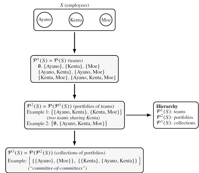
Example 1 (Team groupings via iterated powersets). Let the base set of employees be \[S=\{\mathrm{Ayano},\mathrm{Kenta},\mathrm{Moe}\}.\tag{7}\]
Then \(\mathcal{P}^1(S)=\mathcal{P}(S)\) lists all possible teams: \[\begin{aligned} \mathcal{P}^1(S)=\{&\emptyset,\{\mathrm{Ayano}\},\{\mathrm{Kenta}\},\{\mathrm{Moe}\}, \{\mathrm{Ayano},\mathrm{Kenta}\}, \{\mathrm{Ayano},\mathrm{Moe}\},\{\mathrm{Kenta},\mathrm{Moe}\}, \{\mathrm{Ayano},\mathrm{Kenta},\mathrm{Moe}\}\}. \end{aligned}\tag{8}\]
At the next level, \(\mathcal{P}^2(S)=\mathcal{P}(\mathcal{P}^1(S))\) consists of portfolios of teams. For instance, \[\bigl\{\{\mathrm{Ayano},\mathrm{Kenta}\},\{\mathrm{Kenta},\mathrm{Moe}\}\bigr\}\in \mathcal{P}^2(S),\tag{9}\] selects two teams that share Kenta, while \[\bigl\{\emptyset,\{\mathrm{Ayano},\mathrm{Kenta},\mathrm{Moe}\}\bigr\}\in \mathcal{P}^2(S),\tag{10}\] pairs the empty team with the full task force. At level \(3\), \[\mathcal{P}^3(S)=\mathcal{P}(\mathcal{P}^2(S)),\tag{11}\] collects sets of such portfolios; for example, \[\left\{\{\{\mathrm{Ayano}\},\{\mathrm{Moe}\}\}, \{\{\mathrm{Kenta}\},\{\mathrm{Ayano},\mathrm{Kenta}\}\}\right\}\in \mathcal{P}^3(S).\tag{12}\]
This element can be interpreted as a committee-of-committees description. In summary, iterated powersets naturally encode the levels \[\mathcal{P}^1(S)\ \text{(teams)},\qquad \mathcal{P}^2(S)\ \text{(portfolios of teams)},\qquad \mathcal{P}^3(S)\ \text{(collections of portfolios)}.\tag{13}\]
Figure 1 illustrates this hierarchy.
Definition 2 (Hypergraph [2,17]). A hypergraph is an ordered pair \(H=(V(H),E(H))\) consisting of a nonempty vertex set \(V(H)\) and a family of hyperedges \[E(H)\subseteq \mathcal{P}^{\ast}\bigl(V(H)\bigr).\tag{14}\]
Every hyperedge is a nonempty subset of \(V(H)\) and may contain more than two vertices. Thus a hypergraph generalizes a simple undirected graph by permitting higher-arity incidences.
Definition 3 (\(n\)-Super-HyperGraph). Let \(V_0\) be a finite nonempty base set and let \(n\in\mathbb{N}_{0}\). An \(n\)-Super-HyperGraph over \(V_0\) is a pair \[\mathrm{SHG}^{(n)}=(V,E),\tag{15}\] such that \[V\subseteq \mathcal{P}^n(V_0),\qquad E\subseteq \mathcal{P}^{\ast}(V).\tag{16}\]
Elements of \(V\) are called \(n\)-supervertices. Elements of \(E\) are called \(n\)-superedges; equivalently, each superedge is a nonempty set of \(n\)-supervertices. When \(n=0\), this definition reduces to an ordinary hypergraph \((V,E)\) with \(V\subseteq V_0\) and \(E\subseteq \mathcal{P}^{\ast}(V)\).
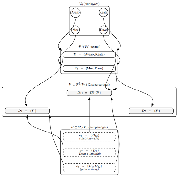
Example 2 (A \(2\)-Super-HyperGraph in corporate project management). Let \[V_0=\{\mathrm{Ayano},\mathrm{Kenta},\mathrm{Moe},\mathrm{Dave}\},\tag{17}\] be the set of employees. Define two first-level teams \[T_1:=\{\mathrm{Ayano},\mathrm{Kenta}\},\qquad T_2:=\{\mathrm{Moe},\mathrm{Dave}\},\tag{18}\] so that \(T_1,T_2\in\mathcal{P}^1(V_0)=\mathcal{P}(V_0)\). At the next level, define \[D_1:=\{T_1\},\qquad D_2:=\{T_2\},\qquad D_{12}:=\{T_1,T_2\},\tag{19}\] so \(D_1,D_2,D_{12}\in\mathcal{P}^2(V_0)\). A \(2\)-Super-HyperGraph is then \[V:=\{D_1,D_2,D_{12}\}\subseteq \mathcal{P}^2(V_0),\qquad E:=\bigl\{\{D_{12}\},\{D_1\},\{D_1,D_{12}\}\bigr\}\subseteq \mathcal{P}^{\ast}(V).\tag{20}\]
Here \(D_{12}\) represents the division consisting of both teams, \(D_1\) represents the first team viewed as a second-level unit, and the superedges represent division-wide, team-internal, and joint activities. The resulting hierarchy is \[\text{employees }(V_0)\longrightarrow \text{teams }(\mathcal{P}^1(V_0))\longrightarrow \text{division units }(\mathcal{P}^2(V_0)).\tag{21}\]
Figure 2 gives a schematic view.
Temporal graphs model pairwise relations whose activity changes over time [11,19].
Definition 4 (Temporal graph). A finite undirected temporal graph is a quadruple \[G=(V,E,T,\lambda),\tag{22}\] where
\(V\) is a finite set of vertices;
\(E\subseteq \{\{u,v\}\subseteq V\mid u\neq v\}\) is a finite set of potential edges;
\(T\) is a nonempty time domain, either a subset of \(\mathbb{R}\) with the inherited order or a discrete totally ordered set;
\(\lambda:E\to 2^T\) assigns to each edge \(e\in E\) the set \(\lambda(e)\subseteq T\) of time points at which \(e\) is active.
For each \(t\in T\), the snapshot graph at time \(t\) is \[G(t)=(V,E(t)),\qquad E(t)=\{e\in E\mid t\in\lambda(e)\}.\tag{23}\]
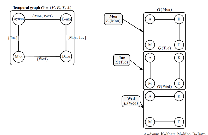
Example 3 (Office co-working temporal graph). Let \[V=\{\mathrm{Ayano},\mathrm{Kenta},\mathrm{Moe},\mathrm{Dave}\},\tag{24}\] and \[E=\bigl\{\{\mathrm{Ayano},\mathrm{Kenta}\},\{\mathrm{Ayano},\mathrm{Moe}\}, \{\mathrm{Kenta},\mathrm{Dave}\},\{\mathrm{Moe},\mathrm{Dave}\}\bigr\}.\tag{25}\]
For the time domain \(T=\{\mathrm{Mon},\mathrm{Tue},\mathrm{Wed}\}\), define \[\begin{aligned} \lambda(\{\mathrm{Ayano},\mathrm{Kenta}\})&=\{\mathrm{Mon},\mathrm{Wed}\}, & \lambda(\{\mathrm{Ayano},\mathrm{Moe}\})&=\{\mathrm{Tue}\},\notag\\ \lambda(\{\mathrm{Kenta},\mathrm{Dave}\})&=\{\mathrm{Mon},\mathrm{Tue}\}, & \lambda(\{\mathrm{Moe},\mathrm{Dave}\})&=\{\mathrm{Wed}\}. \end{aligned}\tag{26}\]
The Monday snapshot has \[E(\mathrm{Mon})=\bigl\{\{\mathrm{Ayano},\mathrm{Kenta}\},\{\mathrm{Kenta},\mathrm{Dave}\}\bigr\}.\tag{27}\]
Figure 3 illustrates the temporal graph and its daily snapshots.
A temporal hypergraph tracks multi-way hyperedges over time by assigning activation times to each potential hyperedge [12–14].
Definition 5 (Temporal hypergraph). A temporal hypergraph is a quadruple \[H=(V,\mathcal E,T,\rho),\tag{28}\] where
\(V\) is a finite vertex set;
\(\mathcal E\subseteq \mathcal{P}^{\ast}(V)\) is a finite set of potential hyperedges;
\(T\) is a nonempty time domain, either a subset of \(\mathbb{R}\) with the inherited order or a discrete totally ordered set;
\(\rho:\mathcal E\to 2^T\) assigns to each hyperedge \(e\in\mathcal E\) the set \(\rho(e)\subseteq T\) of times at which \(e\) is active.
For each \(t\in T\), the snapshot hypergraph at time \(t\) is \[H(t)=(V,\mathcal E(t)),\qquad \mathcal E(t)=\{e\in\mathcal E\mid t\in\rho(e)\}.\tag{29}\]
Example 4 (Office project-team temporal hypergraph). Consider five employees \[V=\{\mathrm{Ayano},\mathrm{Kenta},\mathrm{Moe},\mathrm{Dave},\mathrm{Eva}\},\tag{30}\] and three project teams \[\mathcal E=\bigl\{\{\mathrm{Ayano},\mathrm{Kenta},\mathrm{Moe}\}, \{\mathrm{Kenta},\mathrm{Dave},\mathrm{Eva}\}, \{\mathrm{Ayano},\mathrm{Moe},\mathrm{Eva}\}\bigr\}.\tag{31}\]
Let \(T=\{\mathrm{Week}_1,\mathrm{Week}_2,\mathrm{Week}_3,\mathrm{Week}_4\}\) and define \[\begin{aligned} \rho(\{\mathrm{Ayano},\mathrm{Kenta},\mathrm{Moe}\})&=\{\mathrm{Week}_1,\mathrm{Week}_3\},\notag\\ \rho(\{\mathrm{Kenta},\mathrm{Dave},\mathrm{Eva}\})&=\{\mathrm{Week}_2,\mathrm{Week}_4\},\notag\\ \rho(\{\mathrm{Ayano},\mathrm{Moe},\mathrm{Eva}\})&=\{\mathrm{Week}_1,\mathrm{Week}_4\}. \end{aligned}\tag{32}\]
Then \(H=(V,\mathcal E,T,\rho)\) is a temporal hypergraph. In Week 1, \[\mathcal E(\mathrm{Week}_1)=\bigl\{\{\mathrm{Ayano},\mathrm{Kenta},\mathrm{Moe}\}, \{\mathrm{Ayano},\mathrm{Moe},\mathrm{Eva}\}\bigr\},\tag{33}\] so two multi-person project teams are active in that week.
This section defines temporal Super-HyperGraphs and establishes their basic structural properties. The central idea is to place temporal activity on superedges while keeping the hierarchical supervertex domain explicit.
Definition 6 (Temporal \(n\)-Super-HyperGraph). Let \(V_0\) be a finite nonempty base set, and define iterated powersets by \[\mathcal{P}^0(V_0)=V_0, \qquad \mathcal{P}^{k+1}(V_0)=\mathcal{P}\bigl(\mathcal{P}^k(V_0)\bigr) \quad (k\geq 0).\tag{34}\]
Fix \(n\in\mathbb{N}_{0}\). A temporal \(n\)-Super-HyperGraph over \(V_0\) is a quadruple \[\mathrm{TnSHG}^{(n)}=(V,E,T,\Lambda),\tag{35}\] such that \[\emptyset\neq V\subseteq \mathcal{P}^n(V_0),\qquad E\subseteq \mathcal{P}^{\ast}(V),\tag{36}\] \(T\) is a nonempty time domain, and \[\Lambda:E\longrightarrow 2^T,\tag{37}\] is a time-label function. The set \(\Lambda(e)\subseteq T\) is the activity set of the \(n\)-superedge \(e\in E\). For each \(t\in T\), the snapshot at time \(t\) is \[\mathrm{TnSHG}^{(n)}(t)=(V,E(t)),\qquad E(t)=\{e\in E\mid t\in\Lambda(e)\}.\tag{38}\]
Example 5 (Temporal \(2\)-Super-HyperGraph for software development teams). Let \[V_0=\{\mathrm{Ayano},\mathrm{Kenta},\mathrm{Moe},\mathrm{Dave},\mathrm{Eva}\},\tag{39}\] be a set of engineers. At level \(1\), define \[T_1=\{\mathrm{Ayano},\mathrm{Kenta},\mathrm{Moe}\},\qquad T_2=\{\mathrm{Dave},\mathrm{Eva}\}.\tag{40}\]
At level \(2\), define \[D_1=\{T_1\},\qquad D_2=\{T_2\},\qquad D_{12}=\{T_1,T_2\},\tag{41}\] and let \[V=\{D_1,D_2,D_{12}\}\subseteq \mathcal{P}^2(V_0), \qquad E=\bigl\{\{D_{12}\},\{D_1\}\bigr\}\subseteq \mathcal{P}^{\ast}(V).\tag{42}\]
The superedge \(\{D_{12}\}\) represents a division-wide project, while \(\{D_1\}\) represents a team-internal initiative. For \[T=\{\mathrm{Week}_1,\mathrm{Week}_2,\mathrm{Week}_3\},\tag{43}\] define \[\Lambda(\{D_{12}\})=\{\mathrm{Week}_1,\mathrm{Week}_2\}, \qquad \Lambda(\{D_1\})=\{\mathrm{Week}_1,\mathrm{Week}_3\}.\tag{44}\]
Then \(\mathrm{TnSHG}^{(2)}=(V,E,T,\Lambda)\) records both the team-division hierarchy and the weeks during which each higher-level initiative is active. For example, \[E(\mathrm{Week}_2)=\bigl\{\{D_{12}\}\bigr\},\tag{45}\] so only the division-wide project is active in Week 2.
Example 6 (Temporal \(2\)-Super-HyperGraph for warehouse distribution). Let \[V_0=\{W_1,W_2,W_3,W_4\},\tag{46}\] be a set of warehouses. Define regional clusters \[C_1=\{W_1,W_2\},\qquad C_2=\{W_3,W_4\},\tag{47}\] and second-level supervertices \[N_1=\{C_1\},\qquad N_2=\{C_2\},\qquad N_{12}=\{C_1,C_2\}.\tag{48}\]
Let \[V=\{N_1,N_2,N_{12}\}\subseteq \mathcal{P}^2(V_0), \qquad E=\bigl\{\{N_1\},\{N_2\},\{N_1,N_2\}\bigr\}.\tag{49}\]
The singleton superedges represent intra-region shipments, while \(\{N_1,N_2\}\) represents cross-region shipments. For \[T=\{\mathrm{Day}_1,\mathrm{Day}_2,\mathrm{Day}_3\},\tag{50}\] let \[\begin{aligned} \begin{cases} \Lambda(\{N_1\})=\{\mathrm{Day}_1,\mathrm{Day}_3\},\\ \Lambda(\{N_2\})=\{\mathrm{Day}_1,\mathrm{Day}_2\},\\ \Lambda(\{N_1,N_2\})=\{\mathrm{Day}_2,\mathrm{Day}_3\}.\end{cases} \end{aligned}\tag{51}\]
Then \[E(\mathrm{Day}_2)=\bigl\{\{N_2\},\{N_1,N_2\}\bigr\},\tag{52}\] which means that intra-region shipments in the second cluster and cross-region shipments are active on Day 2.
Example 7 (Temporal \(2\)-Super-HyperGraph for smart building control). Let \[V_0=\{s_1,s_2,s_3,s_4,s_5,s_6,s_7,s_8\},\tag{53}\] be a set of temperature sensors. The sensors are grouped by room: \[R_1=\{s_1,s_2\},\quad R_2=\{s_3,s_4\},\quad R_3=\{s_5,s_6\},\quad R_4=\{s_7,s_8\}.\tag{54}\]
Rooms form floors \[F_1=\{R_1,R_2\},\qquad F_2=\{R_3,R_4\},\tag{55}\] and the \(2\)-supervertex set is \[V=\{F_1,F_2\}\subseteq \mathcal{P}^2(V_0).\tag{56}\]
Let \[E=\bigl\{\{F_1\},\{F_2\},\{F_1,F_2\}\bigr\}.\tag{57}\]
The singleton superedges represent floor-specific control events, while \(\{F_1,F_2\}\) represents a coordinated cross-floor control event. For \[T=\{\mathrm{Morning},\mathrm{Afternoon},\mathrm{Evening}\},\tag{58}\] define \[\begin{aligned} \begin{cases} \Lambda(\{F_1\})=\{\mathrm{Morning},\mathrm{Evening}\},&\\ \Lambda(\{F_2\})=\{\mathrm{Morning},\mathrm{Afternoon}\},&\\ \Lambda(\{F_1,F_2\})=\{\mathrm{Afternoon},\mathrm{Evening}\}.&\end{cases} \end{aligned}\tag{59}\]
In the afternoon, \[E(\mathrm{Afternoon})=\bigl\{\{F_2\},\{F_1,F_2\}\bigr\},\tag{60}\] so the active structure contains both a Floor 2 event and a coordinated cross-floor event.
Theorem 1 (Hierarchy of special cases). Let \(\mathrm{TnSHG}^{(n)}=(V,E,T,\Lambda)\) be a temporal \(n\)-Super-HyperGraph with \(V\subseteq\mathcal{P}^n(V_0)\) and \(E\subseteq\mathcal{P}^{\ast}(V)\). Then the following reductions hold.
(1) If \(T\) and \(\Lambda\) are omitted, the pair \((V,E)\) is a static \(n\)-Super-HyperGraph.
(2) If \(n=0\), then \(V\subseteq V_0\) and \((V,E,T,\Lambda)\) is a temporal hypergraph.
(3) If \(n=0\), \(V=V_0\), and every \(e\in E\) has cardinality \(2\), then \((V,E,T,\Lambda)\) is a temporal graph.
Proof. For (1), the defining conditions \(V\subseteq\mathcal{P}^n(V_0)\) and \(E\subseteq\mathcal{P}^{\ast}(V)\) are exactly the defining conditions of a static \(n\)-Super-HyperGraph once the time domain and time-label function are omitted.
For (2), if \(n=0\), then \(\mathcal{P}^0(V_0)=V_0\), so \(V\subseteq V_0\) and \(E\subseteq\mathcal{P}^{\ast}(V)\). With \(T\) and \(\Lambda:E\to 2^T\), this is precisely a temporal hypergraph, with hyperedge family \(E\) and activity map \(\Lambda\).
For (3), impose in addition \(V=V_0\) and \(E\subseteq\{\{u,v\}\subseteq V_0\mid u\neq v\}\). Then each superedge is a two-element undirected edge, and \(\Lambda(\{u,v\})\) is the set of times at which that edge is active. Hence the quadruple is a temporal graph. \(\square\)
Theorem 2 (Snapshot staticity). Let \(\mathrm{TnSHG}^{(n)}=(V,E,T,\Lambda)\) be a temporal \(n\)-Super-HyperGraph. For each \(t\in T\), define \[E(t)=\{e\in E\mid t\in\Lambda(e)\}.\tag{61}\]
Then \(\mathrm{TnSHG}^{(n)}(t)=(V,E(t))\) is a static \(n\)-Super-HyperGraph on the same supervertex family \(V\).
Proof. Since \(V\subseteq\mathcal{P}^n(V_0)\) by assumption, the vertex condition is unchanged. Also \(E(t)\subseteq E\subseteq\mathcal{P}^{\ast}(V)\), so every element of \(E(t)\) is a nonempty subset of \(V\). Therefore \((V,E(t))\) satisfies the definition of a static \(n\)-Super-HyperGraph. \(\square\)
Theorem 3 (Temporal union and persistent intersection). Let \(\mathrm{TnSHG}^{(n)}=(V,E,T,\Lambda)\) be a temporal \(n\)-Super-HyperGraph over a nonempty time domain \(T\). For each \(t\in T\), let \(E(t)=\{e\in E\mid t\in\Lambda(e)\}\) and define \[E_{\cup}:=\bigcup_{t\in T}E(t),\qquad E_{\cap}:=\bigcap_{t\in T}E(t).\tag{62}\]
Then \((V,E_{\cup})\) and \((V,E_{\cap})\) are static \(n\)-Super-HyperGraphs. The set \(E_{\cup}\) contains the superedges active at least once, while \(E_{\cap}\) contains the superedges active at every time point.
Proof. For each \(t\in T\), \(E(t)\subseteq E\subseteq\mathcal{P}^{\ast}(V)\). Hence \(E_{\cup}\subseteq\mathcal{P}^{\ast}(V)\). Since \(T\) is nonempty, \(E_{\cap}\subseteq E(t_0)\) for any fixed \(t_0\in T\), so \(E_{\cap}\subseteq\mathcal{P}^{\ast}(V)\). In both cases the vertex condition \(V\subseteq\mathcal{P}^n(V_0)\) is unchanged. \(\square\)
Theorem 4 (Time-restriction closure). Let \(\mathrm{TnSHG}^{(n)}=(V,E,T,\Lambda)\) be a temporal \(n\)-Super-HyperGraph, and let \(\emptyset\neq T’\subseteq T\). Define \[\Lambda|_{T’}^{E}:E\longrightarrow 2^{T’},\qquad \Lambda|_{T’}^{E}(e)=\Lambda(e)\cap T’.\tag{63}\]
Then \[\mathrm{TnSHG}^{(n)}|_{T’}=(V,E,T’,\Lambda|_{T’}^{E}),\tag{64}\] is a temporal \(n\)-Super-HyperGraph on the reduced time domain \(T’\).
Proof. The vertex and superedge families are unchanged. Since \(T’\subseteq T\), the set \(T’\) inherits the relevant ordering. For every \(e\in E\), \(\Lambda(e)\cap T’\subseteq T’\), so \(\Lambda|_{T’}^{E}\) is a well-defined map from \(E\) to \(2^{T’}\). \(\square\)
Theorem 5 (Closure under intersection of temporal Super-HyperGraphs). Let \[\mathrm{TnSHG}_1^{(n)}=(V,E_1,T,\Lambda_1),\qquad \mathrm{TnSHG}_2^{(n)}=(V,E_2,T,\Lambda_2),\tag{65}\] be temporal \(n\)-Super-HyperGraphs with the same vertex family \(V\) and time domain \(T\). Define \[E_{\cap}=E_1\cap E_2, \qquad \Lambda_{\cap}(e)=\Lambda_1(e)\cap\Lambda_2(e)\quad (e\in E_{\cap}).\tag{66}\]
Then \[\mathrm{TnSHG}_{\cap}^{(n)}=(V,E_{\cap},T,\Lambda_{\cap}),\tag{67}\] is a temporal \(n\)-Super-HyperGraph.
Proof. Because \(E_1,E_2\subseteq\mathcal{P}^{\ast}(V)\), their intersection is also a subset of \(\mathcal{P}^{\ast}(V)\). For each \(e\in E_{\cap}\), both \(\Lambda_1(e)\) and \(\Lambda_2(e)\) are subsets of \(T\), so \(\Lambda_{\cap}(e)\subseteq T\). Therefore \(\Lambda_{\cap}:E_{\cap}\to 2^T\) is well-defined, and the defining conditions are satisfied. \(\square\)
Theorem 6 (Closure under union of temporal Super-HyperGraphs). Let \[\mathrm{TnSHG}_1^{(n)}=(V,E_1,T,\Lambda_1),\qquad \mathrm{TnSHG}_2^{(n)}=(V,E_2,T,\Lambda_2),\tag{68}\] be temporal \(n\)-Super-HyperGraphs with the same vertex family \(V\) and time domain \(T\). Define \[E_{\cup}=E_1\cup E_2,\tag{69}\] and \(\Lambda_{\cup}:E_{\cup}\to 2^T\) by \[\Lambda_{\cup}(e)= \begin{cases} \Lambda_1(e)\cup\Lambda_2(e), & e\in E_1\cap E_2,\\ \Lambda_1(e), & e\in E_1\setminus E_2,\\ \Lambda_2(e), & e\in E_2\setminus E_1. \end{cases}\tag{70}\]
Then \[\mathrm{TnSHG}_{\cup}^{(n)}=(V,E_{\cup},T,\Lambda_{\cup}),\tag{71}\] is a temporal \(n\)-Super-HyperGraph.
Proof. The union \(E_{\cup}\) is a subset of \(\mathcal{P}^{\ast}(V)\) because each element belongs to \(E_1\) or \(E_2\). The three cases in the definition of \(\Lambda_{\cup}\) form a disjoint partition of \(E_{\cup}\), so the function is well-defined. In every case, \(\Lambda_{\cup}(e)\) is a subset of \(T\). The vertex family and time domain are unchanged, and all defining conditions follow. \(\square\)
Theorem 7 (Complementation of activity). Let \(\mathrm{TnSHG}^{(n)}=(V,E,T,\Lambda)\) be a temporal \(n\)-Super-HyperGraph. Define \[\Lambda^c(e):=T\setminus\Lambda(e)\qquad(e\in E).\tag{72}\]
Then \[\mathrm{TnSHG}_c^{(n)}=(V,E,T,\Lambda^c),\tag{73}\] is a temporal \(n\)-Super-HyperGraph.
Proof. The vertex family, superedge family, and time domain are unchanged. Since \(\Lambda(e)\subseteq T\), the complement \(T\setminus\Lambda(e)\) is also a subset of \(T\). Thus \(\Lambda^c:E\to 2^T\) is well-defined. \(\square\)
Theorem 8 (Time-shift invariance). Let \(\mathrm{TnSHG}^{(n)}=(V,E,T,\Lambda)\) be a temporal \(n\)-Super-HyperGraph with \(T\subseteq\mathbb{R}\), or with \(T\) a discrete subset of \(\mathbb{R}\). Fix \(s\in\mathbb{R}\) and define \[T_s:=\{t+s\mid t\in T\}\subseteq\mathbb{R}, \qquad \Lambda_s(e):=\{t+s\mid t\in\Lambda(e)\}.\tag{74}\]
Then \[\mathrm{TnSHG}_s^{(n)}=(V,E,T_s,\Lambda_s),\tag{75}\] is a temporal \(n\)-Super-HyperGraph on the shifted time domain \(T_s\).
Proof. The vertex and superedge families are unchanged. The map \(\phi_s:T\to T_s\), \(\phi_s(t)=t+s\), is a bijection and preserves the order inherited from \(\mathbb{R}\). Hence \(T_s\) is an admissible time domain. For each \(e\in E\), \(\Lambda_s(e)\subseteq T_s\), so \(\Lambda_s:E\to 2^{T_s}\) is well-defined. \(\square\)
This section gives a basic construction algorithm for temporal \(n\)-Super-HyperGraphs from a finite family of static snapshots indexed by discrete time points. The algorithm is useful when observations are available as a sequence of static \(n\)-Super-HyperGraphs and one wants a single temporal structure with explicit activity labels.
Fix a finite base set \(V_0\) and an integer \(n\geq 0\). For each time \(t\) in a finite time set \(T\), suppose that a static \(n\)-Super-HyperGraph is given: \[\mathrm{SHG}_t^{(n)}=(V_t,E_t),\tag{76}\] where \[V_t\subseteq\mathcal{P}^n(V_0),\qquad E_t\subseteq\mathcal{P}^{\ast}(V_t)\qquad (t\in T).\tag{77}\]
The goal is to construct a temporal \(n\)-Super-HyperGraph \[\mathrm{TnSHG}^{(n)}=(V,E,T,\Lambda),\tag{78}\] such that \(V\) contains every supervertex observed in at least one input snapshot, \(E\) contains every superedge observed in at least one input snapshot, and \(\Lambda(e)\) records the times at which \(e\) appears. The global vertex family is \[V=\bigcup_{t\in T}V_t,\tag{79}\] so a snapshot \((V,E(t))\) retains the common ambient vertex family. Its active edge set matches \(E_t\); inactive vertices are retained in the ambient domain in the standard temporal-network sense.
Algorithm 1 constructs the temporal structure. In implementation, \(V\) and \(E\) may be represented by hash-based or balanced-tree containers. The map \(\Lambda\) may be represented as a dictionary keyed by a canonical encoding of superedges.
Algorithm 1: Construction of a temporal \(n\)-Super-HyperGraph from static snapshots
Input: Finite base set \(V_0\); integer \(n\geq 0\); finite time set \(T\); for each \(t\in T\), a static \(n\)-Super-HyperGraph \(\mathrm{SHG}_t^{(n)}=(V_t,E_t)\) with \(V_t\subseteq\mathcal{P}^n(V_0)\) and \(E_t\subseteq\mathcal{P}^{\ast}(V_t)\).
Output: Temporal \(n\)-Super-HyperGraph \(\mathrm{TnSHG}^{(n)}=(V,E,T,\Lambda)\).
Initialize \(V \leftarrow \emptyset\) and \(E \leftarrow \emptyset\);
Initialize an associative map \(\Lambda\) with no defined keys;
foreach \(t \in T\) do
\(V \leftarrow V \cup V_t\);
foreach \(e \in E_t\) do
if \(e \notin E\) then
insert \(e\) into \(E\);
set \(\Lambda(e) \leftarrow \emptyset\);
\(\Lambda(e) \leftarrow \Lambda(e) \cup \{t\}\);
return \((V,E,T,\Lambda)\);
Theorem 9 (Correctness of Algorithm 1). Let \(V_0\), \(n\), \(T\), and the family \(\{\mathrm{SHG}_t^{(n)}=(V_t,E_t)\}_{t\in T}\) satisfy the assumptions above, and let \((V,E,T,\Lambda)\) be the output of Algorithm 1. Then:
(1) \(V\subseteq\mathcal{P}^n(V_0)\) and \(E\subseteq\mathcal{P}^{\ast}(V)\), so \((V,E)\) is a static \(n\)-Super-HyperGraph.
(2) \((V,E,T,\Lambda)\) is a temporal \(n\)-Super-HyperGraph.
(3) For every \(t\in T\), the active edge set \(E(t)=\{e\in E\mid t\in\Lambda(e)\}\) satisfies \(E(t)=E_t\).
Proof. For (1), the algorithm constructs \(V=\bigcup_{t\in T}V_t\). Since every \(V_t\) is a subset of \(\mathcal{P}^n(V_0)\), their union is also a subset of \(\mathcal{P}^n(V_0)\). The set \(E\) is formed only by inserting elements from some \(E_t\). If \(e\in E_t\), then \(e\in\mathcal{P}^{\ast}(V_t)\), so \(e\) is nonempty and \(e\subseteq V_t\subseteq V\). Hence \(E\subseteq\mathcal{P}^{\ast}(V)\).
For (2), every key inserted into \(\Lambda\) is an element of \(E\), and each assignment adds a time point from \(T\). Therefore \(\Lambda(e)\subseteq T\) for all \(e\in E\), so \(\Lambda:E\to 2^T\) is well-defined. Together with (1), this proves that \((V,E,T,\Lambda)\) is a temporal \(n\)-Super-HyperGraph.
For (3), fix \(t^\ast\in T\). If \(e\in E_{t^\ast}\), then the iteration at time \(t^\ast\) processes \(e\) and updates \(\Lambda(e)\) by adding \(t^\ast\). Thus \(e\in E(t^\ast)\), and \(E_{t^\ast}\subseteq E(t^\ast)\). Conversely, if \(e\in E(t^\ast)\), then \(t^\ast\in\Lambda(e)\). The only operation that adds \(t^\ast\) to an activity set occurs while processing an edge in \(E_{t^\ast}\), so \(e\in E_{t^\ast}\). Hence \(E(t^\ast)\subseteq E_{t^\ast}\), and equality follows. \(\square\)
Theorem 10 (Time and space complexity of Algorithm 1). Let \[N_V:=\sum_{t\in T}|V_t|, \qquad N_E:=\sum_{t\in T}|E_t|.\tag{80}\]
Assume that membership tests, insertions, and dictionary operations have constant expected time under a canonical representation of supervertices and superedges. Then Algorithm 1 runs in expected time \(O(N_V+N_E)\) and uses space \(O(|V|+|E|+N_E)\).
Proof. Each supervertex in each \(V_t\) is considered once when forming \(V\), giving total expected cost \(O(N_V)\). Each superedge in each \(E_t\) is considered once in the inner loop, and each membership test, insertion, initialization, and singleton insertion into \(\Lambda(e)\) has constant expected cost. This gives total expected edge-processing cost \(O(N_E)\).
The sets \(V\) and \(E\) require \(O(|V|+|E|)\) space. The map \(\Lambda\) stores one pair \((e,t)\) for each occurrence of an edge \(e\in E_t\), so the total size of all activity sets is \(O(N_E)\). The total space is therefore \(O(|V|+|E|+N_E)\). \(\square\)
The proposed model is useful when hierarchy and temporal activity are inseparable. In project management, base vertices can represent individual workers, first-level supervertices can represent teams, and second-level supervertices can represent departments or portfolios. A time-labeled superedge then records when a higher-level task, review process, or coordination event is active. The information retained is not merely which individuals participate, but also which organizational units are involved.
In logistics, warehouses, regional clusters, and distribution networks naturally occupy different structural levels. Temporal superedges distinguish intra-region flows from cross-region flows and identify the days or periods when each flow is active. In smart building control, sensors, rooms, floors, and whole-building control units are nested objects; temporal superedges describe control events that activate at one level or across levels. These examples show that the model preserves a distinction that ordinary temporal hypergraphs may erase after flattening: two interactions can involve the same base elements while differing in the higher-level units through which they occur.
The closure results also have practical meaning. Time restriction supports analysis over a selected observation window. Temporal union combines activity from two sources or two measurement periods. Temporal intersection identifies activity common to multiple structures or persistent across all times. Activity complementation describes inactivity intervals, and time shifts allow comparison of the same structure under a translated schedule. These operations preserve the defining conditions of temporal Super-HyperGraphs, so they can be applied without leaving the model class.
The robustness established here is structural rather than empirical. Small changes in the time-label function \(\Lambda\), such as adding or removing a finite number of active time points, affect only the corresponding snapshot edge sets \[E(t)=\{e\in E\mid t\in\Lambda(e)\}.\tag{81}\]
The hierarchical domain \[V\subseteq\mathcal{P}^n(V_0),\tag{82}\] remains unchanged as long as the base structure is fixed. Hence perturbing temporal activity may modify which superedges are active at selected times, but it does not invalidate the temporal \(n\)-Super-HyperGraph.
The theorems in §3 give a minimal stability guarantee under natural operations: restricting time, combining structures, intersecting activity, complementing activity, and shifting time all produce valid temporal Super-HyperGraphs. Table 3 summarizes the difference between a static Super-HyperGraph and its temporal counterpart.
| Aspect | Static Super-HyperGraph | Temporal Super-HyperGraph |
|---|---|---|
| Core object | \(\mathrm{SHG}^{(n)}=(V,E)\) | \(\mathrm{TnSHG}^{(n)}=(V,E,T,\Lambda)\) |
| Vertex domain | \(V\subseteq\mathcal{P}^n(V_0)\) | Same hierarchical vertex domain, usually fixed across time |
| Edge domain | \(E\subseteq\mathcal{P}^{\ast}(V)\) | Same potential superedge family with temporal activation |
| Time component | None | Explicit nonempty time domain \(T\) |
| Edge activity | A superedge in \(E\) is present in the static structure | A superedge \(e\) is active at \(t\) exactly when \(t\in\Lambda(e)\) |
| Snapshot view | Not applicable | \(\mathrm{TnSHG}^{(n)}(t)=(V,E(t))\), where \(E(t)=\{e\in E\mid t\in\Lambda(e)\}\) |
| Primary information retained | Hierarchical multi-way relations | Hierarchical multi-way relations together with their temporal activity |
This paper defined temporal \(n\)-Super-HyperGraphs as time-labeled higher-order structures over iterated powerset vertex domains. The model retains the identity of hierarchical objects while recording when superedges are active. This combination distinguishes interactions among higher-level units from flattened interactions among their base elements.
The main results show that temporal Super-HyperGraphs contain static Super-HyperGraphs, temporal hypergraphs, and temporal graphs as special cases. Each snapshot is a well-defined static \(n\)-Super-HyperGraph, and the class is preserved by time restriction, temporal union, temporal intersection, activity complementation, and time shifting. The construction algorithm from static snapshots further shows how a temporal structure can be assembled from observed time-indexed data while preserving the input active edge sets.
The study contributes a mathematically consistent model for dynamic higher-order systems in which hierarchy and time cannot be separated. Its immediate implications are conceptual and methodological: it clarifies what information is lost by flattening hierarchical interactions and provides stable operations for analyzing time-dependent superedges. Further computational work can develop traversal algorithms, centrality measures, learning methods, and application-specific validation for temporal Super-HyperGraphs, including variants with fuzzy, soft, hypersoft, neutrosophic, or plithogenic uncertainty descriptions [20–27].