Open Access Full-Text PDF

Open Journal of Mathematical Analysis

Forgotten Polynomial and Forgotten Index of Certain Interconnection Networks

Hajra Siddiqui\(^{1}\), Mohammad Reza Farahani
Department of Mathematics and Statistics University of Lahore Pakistan.; (H. S)
Department of Applied Mathematics of Iran University of Science and Technology, (IUST) Narmak, Tehran 16844, Iran.; (M. R. F)
\(^{1}\)Corresponding Author;  hajraasiddiqui3@gmail.com
Copyright © 2017 Hajra Siddiqui, Mohammad Reza Farahani. This is an open access article distributed under the Creative Commons Attribution License, which permits unrestricted use, distribution, and reproduction in any medium, provided the original work is properly cited.

Abstract

Chemical reaction network theory is an area of applied mathematics that attempts to model the behavior of real world chemical systems. Since its foundation in the 1960s, it has attracted a growing research community, mainly due to its applications in biochemistry and theoretical chemistry. It has also attracted interest from pure mathematicians due to the interesting problems that arise from the mathematical structures involved. It is experimentally proved that many properties of the chemical compounds and their topological indices are correlated. In this report, we compute closed form of forgotten polynomial and forgotten index for interconnection networks. Moreover we give graphs to see dependence of our results on the parameters of structures.

Keywords:

Forgotten polynomial; Topological index; Interconnection networks.

1. Prelimaniries

In mathematical chemistry, mathematical tools such as polynomials and numbers predict properties of compounds without using quantum mechanics. These tools, in combination, capture information hidden in the symmetry of molecular graphs. Most commonly known invariants of such kinds are degree-based topological indices. These are the numerical values that correlate the structure with various physical properties, chemical reactivity and biological activities [1, 2, 3, 4, 5]. It is an established fact that many properties such as heat of formation, boiling point, strain energy, rigidity and fracture toughness of a molecule are strongly connected to its graphical structure and this fact plays a synergic role in chemical graph theory.

The butterfly graphs are considered as the principal graphs of FFT(Fast Fourier Transforms) networks and it is efficient in performing FFT. In butterfly networks the series of switch stages and interconnection patterns that allow \(n\) inputs and \(n\) outputs to be inter linked with each other. The Benes network is comprises of continues butterflies and is known as permutation routing whereas butterfly network is identified as Fast Fourier transforms [6]. Butterfly network and Benes network contains important multistage interconnection networks that comprises of attractive topologies for communication networks [7]. Further these topologies are helpful in parallel computing systems which are IBM,SP1/SP2, MIT transit project, internal structures of optical couplers [8, 9 ].

For the connection of numerous homogenously replicated processes multiprocessor interconnection networks are important which is also called a processing node. Message passing is mostly used for the management and communication between processing nodes for program execution. Planning and using of multiprocessor interconnection networks have significant consideration due to the availability of powerful microprocessors and memory chips [10]. For the extreme parallel computing, multipurpose interconnection mesh networks are widely known. This is the fact that these networks having topologies which reproduce the communication pattern of a wide variety regarding natural problems. Mesh networks have recently received a lot of attention for better scalability to larger networks as compared to hyper cubes [11].

A graph with vertex set \(V(G)\) and edge set \(E(G)\) is connected, if there exist a connection between any pair of vertices in \(G\). The distance between two vertices \(u\) and \(v\) is denoted as \(d(u,v)\) and is the length of shortest path between \(u\) and \(v\) in graph \(G\). The number of vertices of \(G\), adjacent to a given vertex \(v\), is the \emph{degree} of this vertex, and will be denoted by \(d_{v}\). For details on basics of graph theory, any standard text such as [12] can be of great help.

The topological index of a molecule structure can be considered as a non-empirical numerical quantity which quantifies the molecular structure and its branching pattern in many ways. In this point of view, the topological index can be regarded as a score function which maps each molecular structure to a real number and is used as a descriptor of the molecule under testing. Topological indices [13, 14, 15, 16, 17, 18, 19, 20, 21, 22] gives a good predictions of variety of physico-chemical properties of chemical compounds containing boiling point, heat of evaporation, heat of formation, chromatographic retention times, surface tension, vapor pressure etc. Since the 1970s, two degree based graph invariants have been extensively studied. These are the first Zagreb index \(M_{1}\) and the second Zagreb index \(M_{2}\) [23, 24] and defined as: \(M_{1}(G)=\sum\limits_{v\in V(G)}(d_{v})^2\) and \(M_{2}(G)=\sum\limits_{usv\in V(G)}d_{u}d_{v}\).

In this article, we compute closed form of the forgotten polynomial for interconnection networks. We also computed forgotten index of these networks. For detailed study about degree-based topological indices, we refer [25, 26, 27, 28, 29, 30] and the references therein.

2. Mesh derived Networks

There are various open problems suggested for various interconnection networks. To quote Stojmenovic [27]: Designing new architectures remains an area of intensive investigation given that there is no clear winner among existing ones. Let the graph \(G\) shown in figure \(1\)

Figure 1.Graph \(G\)

The stellation of \(G\) is denoted by \(St(G)\) and can be obtained by adding a vertex in each face of \(G\) and then by join these vertices to all vertices

Figure 2. Stellation of G(dotted)

The dual \(Du(G)\) of a graph \(G\) is a graph that has a vertex for each face of \(G\). The graph has an edge whenever two faces of \(G\) are separated from each other, and a self-loop when the same face appears on both sides of an edge, see Figure 3. Hence, the number of faces of a graph is equal to the number of edges of its dual

Figure 3. Dual of graph G

In dual graph, if we delete the vertex corresponding to the bounded face of planer graph, which is unique in it, we get bounded dual \(Bdu(G)\) (see Figure 4).

Figure 4. Bounded dual of graph G (dotted)

Given a connected plane graph \(G\), its medial graph \(M(G)\) has a vertex for each edge of \(G\) and an edge between two vertices for each face of \(G\) in which their corresponding edges occur consecutively (see Figure 5).

Figure 5. Medial of G (dotted)

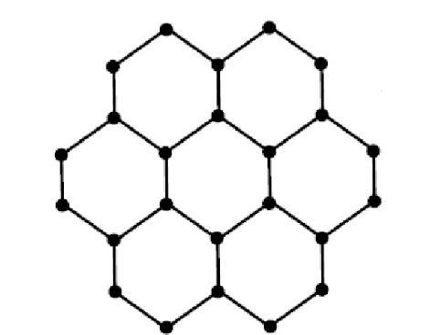
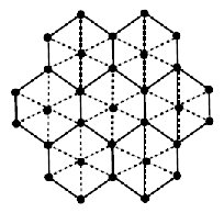
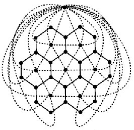
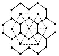
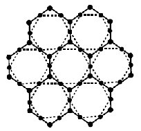
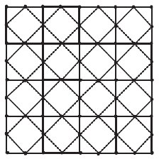
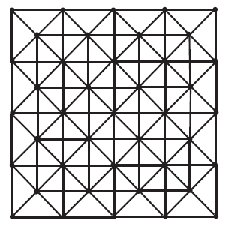
Under this section two new architectures are introduced by using \(m \times n\) mesh network, the defining parameters \(m\) and \(n\) are the number of vertices in any column and row. The restricted dual of Mesh \(m \times n\) is \(m-1 \times n-1\) can be easily noticed. By applying medial operation on mesh \(m{\rm \; \times\; n}\) and deleting the vertex of unrestrained face we found the restricted medial of mesh \(m{\rm \; \times\; n}\). By taking union \(m{\rm \; \times\; n}\) mesh and its restricted medial in a way that the vertices of restricted medial are placed in the middle of each edge of \(m{\rm \; x\; n}\) mesh, the resulting architecture will be the planar named as mesh derived network of first type \(MDN1[m,n]\) network as depicted in Fig. 6. The vertex and edge cardinalities of \(MDN1[m,n]\) network are \(3mn-m-n\) and \(8mn-6(m+n){\rm +}4\) respectively. The second architecture is obtained from the union of \(m{\rm \; \times\; n}\) mesh and its restricted dual \(m-1{\rm \; }\times{\rm \;}n-1\) mesh by joining each vertex of \(m-1{\rm \; }\times{\rm \; }n-1\) mesh to each vertex of parallel face of \(m{\rm \; \times\; n}\) mesh. The resulting architecture will be mesh derived network of second type \(MDN2[m,n]\) network as depicted in Figure 17. The number of vertices and edges of this non planar graph are \(2mn-m-n+1\) and \(8(mn-m-n+1)\) respectively. Some other types of mesh derived networks are well-defined and considered in [31]. The main graph parameter which is discussed in [31] for mesh derived networks is the metric dimension of networks. Now we compute topological indices of these mesh derived networks

Figure 6. MDN1[5, 5] (dotted)

Table 1. Edge partition \(MDN1[m, n]\)

\((d_{u}, d_{v})\) Number of edges
\((2,4)\) \(8\)
\((3,4)\) \(4(m+n-4)\)
\((3,6)\) \(2(m+n-4)\)
\((4,6)\) \(4(mn-n-m)\)
\((4,4)\) \(4\)
\((6,6)\) \(4(mn-2m-2n+4)\)
Theorem 2.1. Let \(MDN1 [m, n]\) is mesh derived networks. Then the Forgotten polynomial and forgotten index of \(MDN1 [m, n]\) are respectively \begin{eqnarray*}F(MDN1[m,n],x)&=&\; 8x^{20} +4(m+n-4)x^{25} +2(m+n-4)x^{45}\\ &&+ 4(mn-m-n)x^{52} + 4x^{32} \\ &&+4(mn-2m-2n+4)x^{72}\end{eqnarray*} \begin{eqnarray*} F(MDN1[m,n])&=&\; 20^{8} \times 25^{4(m+n-4)} \times 45^{2(m+n-4)}\\ &\times& 52^{4(mn-m-n)} \times 32^{4} \times 72^{4(mn-2m-2n+4)} \end{eqnarray*} Proof. From the definition of forgotten polynomial, we have \begin{eqnarray*} F(MDN1[m,n],x)&=&\sum\limits _{uv\in E(MDN1[m,n])}x^{[du^{2} \; +dv^{2} ]} \\ &=&\sum\limits _{uv\in E_{1} (MDN1[m,n])}x^{[du^{2} \; +dv^{2} ]}\\ &&+\sum\limits _{uv\in E_{2} (MDN1[m,n])}x^{[du^{2} \; +dv^{2} ]} \\ &&+\sum\limits _{uv\in E_{3} (MDN1[m,n])}x^{[du^{2} \; +dv^{2} ]} \\ &&+\sum\limits _{uv\in E_{4} (MDN1[m,n])}x^{[du^{2} \; +dv^{2} ]} \\ &&+\sum\limits_{uv\in E_{5} (MDN1[m,n])}x^{[du^{2} \; +dv^{2} ]}\\ &&+\sum\limits_{uv\in E_{6} (MDN1[m,n])}x^{[du^{2} \; +dv^{2} ]} \\ &=& \left|E_{1} (MDN1[m,n])\right|x^{20} +\left|E_{2} (MDN1[m,n])\right|x^{25}\\ && +\left|E_{3} (MDN1[m,n])\right|x^{45}+\left|E_{4} (MDN1[m,n])\right|x^{52}\\ &&+ \left|E_{5} (MDN1[m,n])\right|x^{32} +\left|E_{6} (MDN1[m,n])\right|x^{72} \\ &=&8x^{20} +4(m+n-4)x^{25} +2(m+n-4)x^{45}\\ &&+4(mn-m-n)x^{52}+4x^{32}\\ &&+4(mn-2m-2n+4)x^{72} \end{eqnarray*}

Figure 7. 3D plot of Forgotten Polynomial

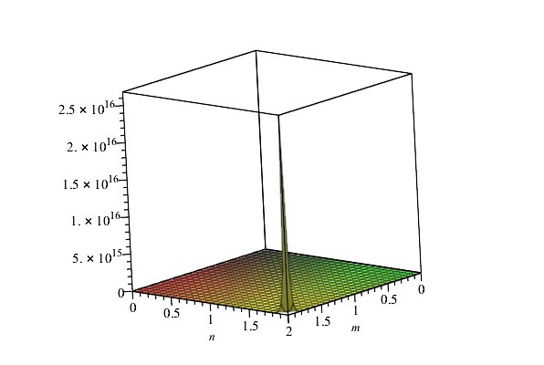
From the definition of forgotten index we have \begin{eqnarray*} F(MDN1[m,n])&=&\prod _{uv\in E(MDN1[m,n])}[du^{2} +dv^{2} ] \\ &=& \prod _{uv\in E_{1} (MDN1[m,n])}[du^{2} +dv^{2} ]\\ &&\times \prod _{uv\in E_{2} (MDN1[m,n])}[du^{2} +dv^{2} ]\\ &&\times \prod _{uv\in E_{3} (MDN1[m,n])}[du^{2} +dv^{2} ] \\ &&\times \prod _{uv\in E_{4} (MDN1[m,n])}[du^{2} +dv^{2} ] \\ &&\times \prod _{uv\in E_{5} (MDN1[m,n])}[du^{2} +dv^{2} ]\\ && \times \prod _{uv\in E_{6} (MDN1[m,n])}[du^{2} +dv^{2} ] \\ &=& 20^{\left|E_{1} (MDN1[m,n])\right|} \times 25^{\left|E_{2} (MDN1[m,n)\right|}\\ &&\times 45^{\left|E_{3} (MDN1[m,n])\right|} \times 52^{\left|E_{4} (MDN1[m,n])\right|}\\ && \times 32^{\left|E_{5} (MDN1[m,n])\right|} \times 72^{\left|E_{6} (MDN1[m,n])\right|} \\ &=& 20^{8} \times 25^{4(m+n-4)} \times 45^{2(m+n-4)} \times 52^{4(mn-m-n)}\\ && \times 32^{4} \times 72^{4(mn-2m-2n+4)} \end{eqnarray*}

Figure 8. 3D plot of Forgotten Index

3. Mesh derived Networks 2

Figure 9. MDN2[m,n]

Table 2. Edge partition MDN2[m, n]
\((d_{u}, d_{v})\) Number of edges
\((3,6)\) \(4\)
\((3,5)\) \(8\)
(5,6) \(8\)
\((5,5)\) \(2(m+n-6)\)
\((6,8)\) 4
\((5,8)\) \(2(m+n-4)\)
\((5,7)\) \(4(m+n-6)\)
\((7,7)\) \(2(m+n-8)\)
\((6,7)\) \(8\)
\((7,8)\) \(6(m+n-6)\)
\((8,8)\) \(8mn-24(m+n)+72\)

Theorem 3.1. Let \(MDN2 [m, n]\) is mesh derived networks. Then the Forgotten Polynomial and Forgotten Index of \(MDN2 [m, n]\) are \begin{eqnarray*} F(MDN2[m,n],x)&=&4x^{45} +8x^{34} +8x^{61} +2(m+n-6)x^{50} +4x^{100} \\ &&+2(m+n-4)x^{89} + 4(m+n-6)x^{74} +2(m+n-8)x^{98}\\ &&+ 8x^{85} +6(m+n-6)x^{113}+(8mn-24(m+n)+72)x^{128} \end{eqnarray*} \begin{eqnarray*} F(MDN2[m,n])&=& 45^{4} \times 34^{8} \times 61^{8} \times 50^{2(m+n-6)} \times 100^{4} \times 89^{2(m+n-4)} \times 74^{4(m+n-6)}\\ &&\times 98^{2(m+n-8)} \times 85^{8} \times 113^{6(m+n-6)} \times 128^{(8mn-24(m+n)+72)} \end{eqnarray*}

Proof. From the definition of Forgotten Polynomial we have \begin{eqnarray*} F(MDN2[m,n],x)\\ &=&\sum _{uv\in E(MDN2[m,n])}x^{[du^{2} \; +dv^{2} ]} \\ &=& \sum _{uv\in E_{1} (MDN2[m,n])}x^{[du^{2} \; +dv^{2} ]} \\ && +\sum _{uv\in E_{2} (MDN2[m,n])}x^{[du^{2} \; +dv^{2} ]} \\ &&+ \sum _{uv\in E_{3} (MDN2[m,n])}x^{[du^{2} \; +dv^{2} ]} \\ &&+ \sum _{uv\in E_{4} (MDN2[m,n])}x^{[du^{2} \; +dv^{2} ]} \\ &&+ \sum _{uv\in E_{5} (MDN2[m,n])}x^{[du^{2} \; +dv^{2} ]} \\ &&+ \sum _{uv\in E_{6} (MDN2[m,n])}x^{[du^{2} \; +dv^{2} ]} \\ &&+ \sum _{uv\in E_{7} (MDN2[m,n])}x^{[du^{2} +dv^{2} ]}\\ &&+\sum _{uv\in E_{8} (MDN2[m,n])}x^{[du^{2} \; +dv^{2} ]} \\ &&+ \sum _{uv\in E_{9} (MDN2[m,n])}x^{[du^{2} \; +dv^{2} ]} \\ && +\; \sum _{uv\in E_{10} (MDN2[m,n])}x^{[du^{2} \; +dv^{2} ]} \\ &&+ \sum _{uv\in E_{11} (MDN2[m,n])}x^{[du^{2} \; +dv^{2} ]}\\ &=& \left|E_{1} (MDN2[m,n])\right|x^{45} +\left|E_{2} (MDN2[m,n])\right|x^{34}\\ &&+ \left|E_{3} (MDN2[m,n])\right|x^{61} +\left|E_{4} (MDN2[m,n])\right|x^{50}\\ &&+\left|E_{5} (MDN2[m,n])\right|x^{100} +\left|E_{6} (MDN2[m,n])\right|x^{89} \\ &&+ \left|E_{7} (MDN2[m,n])\right|x^{74}+\left|E_{8} (MDN2[m,n])\right|x^{98}\\ &&+\left|E_{9} (MDN2[m,n])\right|x^{85} +\left|E_{10} (MDN2[m,n])\right|x^{113}\\ &&+ \left|E_{11} (MDN2[m,n])\right|x^{128} \\ &=& 4x^{45} +8x^{34} +8x^{61} +2(m+n-6)x^{50} \\ &&+4x^{100} +2(m+n-4)x^{89}+ 4(m+n-6)x^{74} \\ &&+2(m+n-8)x^{98}+ 8x^{85} +6(m+n-6)x^{113} \\ &&+(8mn-24(m+n)+72)x^{128} \end{eqnarray*}

Figure 10. 3D plot of forgotten polynomial

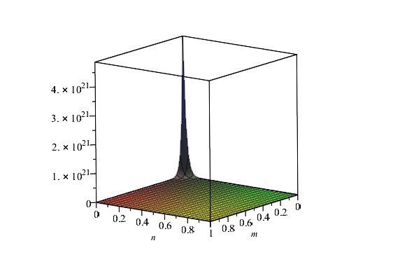
\begin{eqnarray*} F(MDN2[m,n])&=&\prod _{uv\in E(MDN2[m,n])}[du^{2} +dv^{2} ] \\ &=&\prod _{uv\in E_{1} (MDN2[m,n])}[du^{2} +dv^{2} ] \\ &&\times \prod _{uv\in E_{2} (MDN2[m,n])}[du^{2} +dv^{2} ]\\ &&\times \prod _{uv\in E_{3} (MDN2[m,n])}[du^{2} +dv^{2} ]\\ &&\times \prod _{uv\in E_{4} (MDN2[m,n])}[du^{2} +dv^{2} \\ &&\times \; \; \prod _{uv\in E_{5} (MDN2[m,n])}[du^{2} +dv^{2} ] \\ &&\times \prod _{uv\in E_{6} (MDN2[m,n])}[du^{2} +dv^{2} ] \\ &&\times\prod _{uv\in E_{7} (MDN2[m,n])}[du^{2} +dv^{2} ] \\ &&\times \prod _{uv\in E_{8} (MDN2[m,n])}[du^{2} +dv^{2} ]\\ &&\times \prod _{uv\in E_{9} (MDN2[m,n])}[du^{2} +dv^{2} ]\\ &&\times \prod _{uv\in E_{10} (MDN2[m,n])}[du^{2} +dv^{2} ]\\ && \times \prod _{uv\in E_{11} (MDN2[m,n])}[du^{2} +dv^{2} ]\\ &=& 45^{\left|E_{1} (MDN2[m,n])\right|} \times 34^{\left|E_{2} (MDN2[m,n])\right|} \times 61^{\left|E_{3} (MDN2[m,n])\right|}\\ &\times& 50^{\left|E_{4} (MDN2[m,n])\right|} \times 100^{\left|E_{5} (MDN2[m,n])\right|} \\ &\times& 89^{\left|E_{6} (MDN2[m,n])\right|} \times \; 74^{\left|E_{7} (MDN2[m,n])\right|} \times 98^{\left|E_{8} (MDN2[m,n])\right|}\\ &\times& 85^{\left|E_{9} (MDN2[m,n])\right|} \times 113^{\left|E_{10} (MDN2[m,n])\right|} \\ &\times& 128^{\left|E_{11} (MDN2[m,n])\right|}\\ &=& 45^{4} \times 34^{8} \times 61^{8} \times 50^{2(m+n-6)} \\ &\times& 100^{4} \times 89^{2(m+n-4)} \times 74^{4(m+n-6)} \times 98^{2(m+n-8)} \times 85^{8} \\ &\times& 113^{6(m+n-6)} \times 128^{(8mn-24(m+n)+72)} \end{eqnarray*}

Figure 11. 3D plot of forgotten index

4. Butterfly Network

Butterfly network is the most common bounded-degree derivative network of the hypercube. The set \(V\) of vertices of an \(r\)-dimensional butterfly network resemble to pairs \([w, i]\) where \(i\) is the dimension or level of a node \((0\le i\le r)\) and \(w\) is an \(r\)-bit binary number that represents the row of the node. Two nodes \([w,i]\) and \([w',i']\) are connected by an edge if and only if \(\acute{i}=i+1\) and either: \noindent 1. \(w\) and \(w'\) are duplicate, or \noindent 2. \(w\) and \(w'\) differ in specifically the \(i\)-th bit. \noindent Undirected edges are found in the network. An \(r\)-dimensional butterfly network is represented by \(BF(r)\). Manuel et el. [26] offered the diamond representations of these networks. The normal and diamond representations of 3-dimensional butterfly network are given in Figure \(12\). The vertex and edge cardinalities are \(2^{r} (r+1)\) and \(r2^{r+1}\) respectively

Figure 12. Normal representation of butterfly BF(3)

Figure 13. Diamond representation of butterfly BF(3)

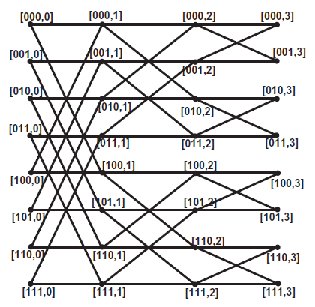
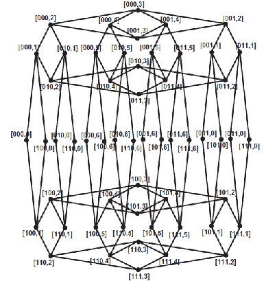
Let \(G=BF(r)\) be the butterfly network. From figure 12, we see that the graph has \(2r(r+1)\) number of vertices and \(r2r+1\) number of edges. The edge partition of graph \(G\) is shown in table 3.

Table 3. Edge partition \(BF(r)\)
\((d_{u}, d_{v})\) Number of edges
\((2,4)\) \(2^{r+2}\)
\((4,4)\) \(2^{r+1}(r-2)\)

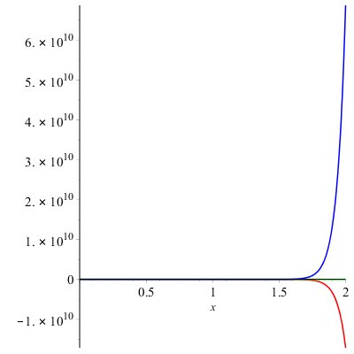
Theorem 4.1. Let \(BF(r)\) is butterfly network then the Forgotten Polynomial and Forgotten Index of \(BF(r)\) are

  1. \(F(BF(r),x)\)= \(2^{r+2} x^{20} +2^{r+1} (r-2)x^{32} \)
  2. \(F(BF(r))\)= \(20^{2^{r+2} } \; \times 32^{2^{r+1} (r-2)} \)

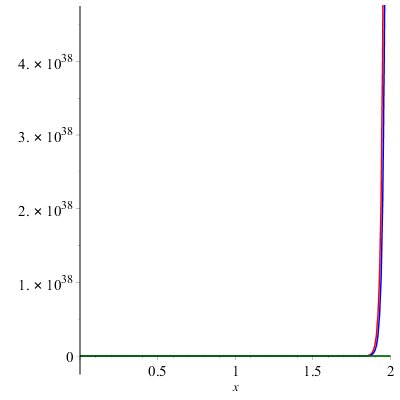
Proof. From the definition of forgotten polynomial we have \begin{eqnarray*} F(BF(r),x)&=&\sum _{uv\in E(BF(r))}x^{[du^{2} \; +dv^{2} ]} \\ &=&\sum _{uv\in E_{1} (BF(r))}x^{[du^{2} \; +dv^{2} ]} +\sum _{uv\in E_{2} (BF(r))}x^{[du^{2} \; +dv^{2} ]} \\ &=& \left|E_{1} (BF(r))\right|x^{20} +\left|E_{2} (BF(r))\right|x^{32} \\ &=& 2^{r+2} x^{20} +2^{r+1} (r-2)x^{32} \end{eqnarray*}

Figure 14. Plot of forgotten polynomial

From the definition of forgotten index we have \begin{eqnarray*} F(BF(r))&=&\prod _{uv\in E(BF(r))}[du^{2} +dv^{2} ] \\ &=& \prod _{uv\in E_{1} (BF(r))}[du^{2} +dv^{2} ] \; \times \prod _{uv\in E_{2} (BF(r))}[du^{2} +dv^{2} ]\\ &=& 20^{\left|E_{1} (BF(r))\right|} \times 32^{\left|E_{2} (BF(r))\right|} \\ &=& 20^{2^{r+2} } \; \times 32^{2^{r+1} (r-2)} \end{eqnarray*}

Figure 15. Plot of forgotten index

5. Benes Network

The \(r\)-dimensional Benes network is continuous butterflies which are represented by \(B_{(r)}\). This \(r\)-dimensional Benes network has levels, each level with \(2r\) nodes. The level \(0\) to level \(r\) nodes in the network form an \(r\)-dimensional butterfly. The middle level of the network is shared by these butterflies. Manuel et al. suggested the diamond representation of the Benes network [32]. Figure 16 shows the normal representation of \(B_{(3)}\) network, while diamond representation of \(B_{(3)}\) is described in Figure 17. The number of vertices and number of edges in an \(r\)-dimensional Benes network are \(2^r(2r+1)\) and \(r2^{r+2}\) respectively.

Figure 16. Normal representation of Bens Network \(B_{(3)}\)

Figure 17. Diamond representation of Bens Network \(B_{(3)}\)

Let be the Benes network. From figure 1, we see that the graph has \(2r(2r+1)\) number of vertices and \(r2^{r+2}\) number of edges. Table 4 shows the edge partition of graph \(G\).
Table 4. Edge partition \(BF(r)\)
\((d_{u}, d_{v})\) Number of edges
\((2,4)\) \(2^{r+2}\)
\((4,4)\) \(2^{r+2}(r-1)\)

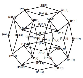
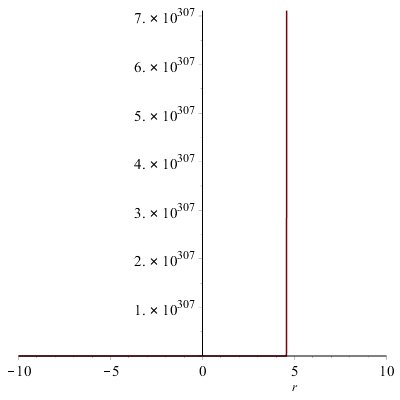
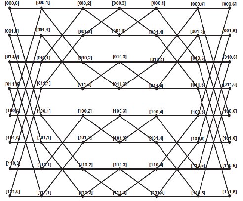
Theorem 5.1. Let \(B_{(r)}\) is Benes network then the Forgotten Polynomial $$F(B_{(r)} ,x)= 2^{r+2} x^{20} +2^{r+2} (r-1)x^{32} $$ and Forgotten Index of \(B_{(r)}\) are $$F(B_{(r)} )= 20^{2^{r+2} } \; \times 32^{2^{r+2} (r-1)} $$

Proof. From the definition of forgotten polynomial we have \begin{eqnarray*} F(B_{(r)} ,x)&=&\sum _{uv\in E(B_{(r)} )}x^{[du^{2} \; +dv^{2} ]} \\ &=&\sum _{uv\in E_{1} (B_{(r)} )}x^{[du^{2} \; +dv^{2} ]} +\sum _{uv\in E_{2} (B_{(r)} )}x^{[du^{2} \; +dv^{2} ]} \\ &=&\left|E_{1} (B_{(r)} )\right|x^{20} +\left|E_{2} (B_{(r)} )\right|x^{32} \\ &=& 2^{r+2} x^{20} +2^{r+2} (r-1)x^{32} \end{eqnarray*}

Figure 18. Plot of forgotten polynomial

From the definition of forgotten index we have \begin{eqnarray*} F(B_{(r)})&=&\prod\limits_{uv\in E(B_{(r)} )}[du^{2} +dv^{2} ] \\ &=& \prod\limits _{uv\in E_{1} (B_{(r)} )}[du^{2} +dv^{2} ] \times \prod\limits _{uv\in E_{2} (B_{(r)} )}[du^{2} +dv^{2} ] \\ &=& 20^{\left|E_{1} (B_{(r)} )\right|} \times 32^{\left|E_{2} (B_{(r)} )\right|} \\ &=& 20^{2^{r+2}} \times 32^{2^{r+2} (r-1)} \end{eqnarray*}

Figure 19. Plot of forgotten index

6. Conclusion

In this article, we have computed Forgotten polynomial and forgotten index for interconnected networks. These indices are actually functions of chemical graphs and encode many chemical properties as viscosity, strain energy, and heat of formation.

Competing Interests

The author do not have any competing interests in the manuscript.

References

  1. Rücker, G., & Rücker, C. (1999). On topological indices, boiling points, and cycloalkanes. Journal of chemical information and computer sciences 39(5), 788-802. [Google Scholor]
  2. Klavžar, S., & Gutman, I. (1996). A comparison of the Schultz molecular topological index with the Wiener index. Journal of chemical information and computer sciences, 36(5), 1001-1003. [Google Scholor]
  3. Brückler, F. M., Došlic, T., Graovac, A., & Gutman, I. (2011). On a class of distance-based molecular structure descriptors. \emph{Chemical physics letters,} 503(4), 336-338. [Google Scholor]
  4. Deng, H., Yang, J., & Xia, F. (2011). A general modeling of some vertex-degree based topological indices in benzenoid systems and phenylenes. Computers & Mathematics with Applications, 61(10), 3017-3023. [Google Scholor]
  5. Zhang, H., \& Zhang, F. (1996). The Clar covering polynomial of hexagonal systems I. Discrete applied mathematics, 69(1-2), 147-167. [Google Scholor]
  6. Beneš, V. E. (Ed.). (1965). Mathematical theory of connecting networks and telephone traffic (Vol. 17). Academic press. [Google Scholor]
  7. Manuel, P. D., Abd-El-Barr, M. I., Rajasingh, I., & Rajan, B. (2008). An efficient representation of Benes networks and its applications. Journal of Discrete Algorithms, 6(1), 11-19. [Google Scholor]
  8. Liu, X. C., & Gu, Q. P. (2002). Multicasts on WDM all-optical butterfly networks. Journal of Information Science and Engineering, 18(6), 1049-1058. [Google Scholor]
  9. Xu, J. (2013). Topological structure and analysis of interconnection networks (Vol. 7). Springer Science & Business Media. [Google Scholor]
  10. Chen, M. S., Shin, K. G., & Kandlur, D. D. (1990). Addressing, routing, and broadcasting in hexagonal mesh multiprocessors. IEEE Transactions on Computers, 39(1), 10-18. [Google Scholor]
  11. Cynthia, V. J. A. (2014). Metric dimension of certain mesh derived graphs. Journal of Computer and Mathematical Sciences, Vol, 5(1), 1-122. [Google Scholor]
  12. West, D. B. (2001). Introduction to graph theory (Vol. 2). Upper Saddle River: Prentice hall . [Google Scholor]
  13. Gutman, I. (1993). Some properties of the Wiener polynomial. Graph Theory Notes of New York, 25, 13-18. [Google Scholor]
  14. Deutsch, E., & Klavžar, S. (2015). M-Polynomial and Degree-Based Topological Indices. Iranian Journal of Mathematical Chemistry, 6(2), 93-102. [Google Scholor]
  15. Munir, M., Nazeer, W., Nizami, A. R., Rafique, S., & Kang, S. M. (2016). M-Polynomials and Topological Indices of Titania Nanotubes. Symmetry, 8(11), 117. [Google Scholor]
  16. Munir, M., Nazeer, W., Rafique, S., & Kang, S. M. (2016). M-polynomial and degree-based topological indices of polyhex nanotubes. Symmetry, 8(12), 149. [Google Scholor]
  17. Ajmal, M., Kang, S. M., Nazeer, W., Munir, M., & Jung, C. Y. (2016). Some Topological Invariants of the Möbius Ladders. Global Journal of Pure and Applied Mathematics, 12(6), 5317-5327. [Google Scholor]
  18. Munir, M., Nazeer, W., Rafique, S., Nizami, A. R., & Kang, S. M. (2017). Some computational aspects of triangular Boron nanotubes. Symmetry , 9(1), 6. [Google Scholor]
  19. Javaid, M., & Jung, C. Y. (2017). M-Polynomials and Topological Indices of Silicate and Oxide Networks. International Journal of Pure and Applied Mathematics , 115 (1) 129-152. [Google Scholor]
  20. Kwun, Y. C., Munir, M., Nazeer, W., Rafique, S., & Kang, S. M. (2017). M-Polynomials and topological indices of V-Phenylenic Nanotubes and Nanotori. Scientific reports , 7(1), 8756. [Google Scholor]
  21. Gutman, I., & Polansky, O. E. (2012). Mathematical concepts in organic chemistry. Springer Science & Business Media. [Google Scholor]
  22. Wiener, H. (1947). Structural determination of paraffin boiling points. Journal of the American Chemical Society, 69(1), 17-20. [Google Scholor]
  23. Gutman, I., & Das, K. C. (2004). The first Zagreb index 30 years after. MATCH Commun. Math. Comput. Chem , 50, 83-92. [Google Scholor]
  24. Das, K. C., & Gutman, I. (2004). Some properties of the second Zagreb index. MATCH Commun. Math. Comput. Chem, 52(1), 3-1. [Google Scholor]
  25. Sardar, M. S, Zafar, S., & Farahani, M. R. (2017). The generalized zagreb index of capra-designed planar benzenoid series \(ca_k(c_6)\), Open J. Math. Sci., 1(1), 44-51. [Google Scholor]
  26. Rehman, H. M, Sardar, R., Raza, A. (2017). computing topological indices of hex board and its line graph. Open J. Math. Sci., 1(1), 62- 71. [Google Scholor]
  27. Farahani, M. R., Gao, W., Baig, A. Q., & Khalid, W. (2017). Molecular description of copper (II) oxide. Macedonian Journal of Chemistry and Chemical Engineering, 36(1), 93-99. [Google Scholor]
  28. Gao, W., Wang, Y., Wang, W., & Shi, L. (2017). The first multiplication atom-bond connectivity index of molecular structures in drugs. Saudi Pharmaceutical Journal, 25(4), 548-555. [Google Scholor]
  29. Gao, W., Farahani, M. R., Wang, S., & Husin, M. N. (2017). On the edge-version atom-bond connectivity and geometric arithmetic indices of certain graph operations. Applied Mathematics and Computation, 308, 11-17. [Google Scholor]
  30. Zomaya, A. Y. (1996). Parallel and distributed computing handbook. [Google Scholor]
  31. Cynthia, V. J. A. (2014). Metric dimension of certain mesh derived graphs. Journal of Computer and Mathematical Sciences, 5(1), 1-122. [Google Scholor]
  32. Manuel, P. D., Abd-El-Barr, M. I., Rajasingh, I., & Rajan, B. (2008). An efficient representation of Benes networks and its applications. Journal of Discrete Algorithms, 6(1), 11-19 [Google Scholor] .