
Jordan’s inequality [1– 6] \[\begin{aligned} \label{eqn1.1} \frac{2}{\pi} \leq \frac{\sin x}{x} < 1; \, \, \, x \in (0, \pi/2], \end{aligned} \tag{1}\] gives bounds for the sinc function which is defined by \(\mathop{\mathrm{sinc}}x = (\sin x)/x,\) if \(x \neq 0\) and \(\mathop{\mathrm{sinc}}x = 1,\) if \(x = 0.\) The double inequality (1) is a consequence of the monotonicity of the curve \(y = \mathop{\mathrm{sinc}}x\) or the concavity of the curve \(y =\sin x\) in \((0, \pi/2].\) It can also be easily achieved through the geometry of circles [7]. Jordan’s inequality has its glory among the trigonometric functions due to its importance in calculus and analysis. This much-appreciated inequality motivated many researchers to obtain its refinements, extensions, and generalizations, see for instance [5, 8– 28] and the references therein. In \(2010,\) Klén et. al. [3] rediscovered the inequality (1) as follows: \[\begin{aligned} \label{eqn1.2} 1 – \frac{x^2}{6} < \frac{\sin x}{x} < 1 – \frac{2x^2}{3\pi^2}; \, \, \, x \in (-\pi/2, \pi/2). \end{aligned} \tag{2}\]
Further, in \(2022,\) Bagul and Panchal [29] improved inequality (2) to \[\begin{aligned} \label{eqn1.3} 1 – \frac{x^2}{6} < \frac{\sin x}{x} < 1 – \frac{4x^2}{3\pi^2}; \, \, \, x \in (-\pi/2, \pi/2). \end{aligned} \tag{3}\]
Recently, the Jordan-type inequalities (2) and (3) have been generalized and explored in detail in [10]. This article aims to contribute to the field by refining the lower and upper bounds of (3). It is worth noting that due to the symmetry of the curves involved, it suffices to improve the inequality (3) in \((0, \alpha)\) rather than in \((-\alpha, \alpha).\) The new sharp bounds are established in terms of bounds of inequality (2) and cosine function.
We begin by recalling the following series expansions [30, 1.411]: \[\begin{aligned} \label{eqn2.1} \frac{x}{\sin x} = 1 + \sum\limits_{k=1}^\infty \frac{2(2^{2k-1}-1)}{(2k)!} \vert B_{2k} \vert x^{2k}; \, \, \, \vert x \vert < \pi, \end{aligned} \tag{4}\] \[\begin{aligned} \label{eqn2.2} \cot x = \frac{1}{x} – \sum\limits_{k=1}^\infty \frac{2^{2k}}{(2k)!} \vert B_{2k} \vert x^{2k-1}; \, \, \, \vert x \vert < \pi, \end{aligned} \tag{5}\] where \(\vert B_{2k} \vert\) are the absolute even-indexed Bernoulli numbers.
Differentiating (5) and then multiplying by \(-x^2\) yields \[\begin{aligned} \label{eqn2.3} \left(\frac{x}{\sin x}\right)^2 = 1 + \sum\limits_{k=1}^\infty \frac{2^{2k}(2k-1)}{(2k)!} \vert B_{2k} \vert x^{2k}; \, \, \, \vert x \vert < \pi. \end{aligned} \tag{6}\]
Also, we will employ the following supplementary results.
Lemma 1.[31, 32](l’Hôpital monotone rule) Suppose \(p\) and \(q\) are any two real numbers such that \(p < q.\) Let \(f_1(x)\) and \(f_2(x)\) be two real-valued functions that are continuous on \([p, q]\) and differentiable on \((p, q)\), and \(f_2^{\prime}(x) \neq 0,\) for all \(x \in (p, q).\) Let, \[i(x) = \frac{f_1(x) – f_1(p)}{f_2(x) – f_2(p)}, \quad j(x) = \frac{f_1(x) – f_1(q)}{f_2(x) – f_2(q)}.\]
Then, the functions \(i(x)\) and \(j(x)\) are increasing (decreasing) on \((p, q)\) if \(f_1^{\prime}(x)/f_2^{\prime}(x)\) is increasing (decreasing) on \((p, q).\) The strictness of the monotonicity of \(i(x)\) and \(j(x)\) depends on the strictness of the monotonicity of \(f_1^{\prime}(x)/f_2^{\prime}(x)\).
The l’Hôpital monotone rule in Lemma 1 has been proven to be an important tool in the field of inequalities. The next lemma concerns the monotonicity of the ratio of two series and can be found in [33].
Lemma 2. [33] Let \(P(x) =\sum\limits_{k=0}^\infty p_k x^k\) and \(Q(x) = \sum\limits_{k=0}^\infty q_k x^k\) be any two real series converging on the interval \((-R, R),\) where \(R > 0\) and \(q_k > 0\) for all \(k.\) Then the function \(P(x)/Q(x)\) is increasing (decreasing) on \((0, R)\) if the sequence \(\left\lbrace {p_k}/q_k \right\rbrace\) is increasing (decreasing).
In addition, we need a double inequality for the ratio of consecutive absolute Bernoulli numbers recently established by Qi [34].
Lemma 3. ([34]) For \(k \in \mathbb{N},\) the Bernoulli numbers satisfy \[\frac{(2^{2k – 1} – 1)}{(2^{2k + 1} – 1)} \frac{(2k + 1) (2k + 2)}{\pi^2} < \frac{\vert B_{2k + 2} \vert}{\vert B_{2k} \vert} < \frac{(2^{2k} – 1)}{(2^{2k + 2} – 1)} \frac{(2k + 1) (2k + 2)}{\pi^2}.\]
We are now in a position to assert our results with their proofs. First, we use the functions \(\left(1-\frac{x^2}{6}\right)\) and \((1-\cos x)^2\) to refine inequalities (3).
Theorem 1. The function \(\left[\frac{\sin x}{x} – \left(1-\frac{x^2}{6}\right)\right] \big/ (1-\cos x)^2\) is strictly increasing from \((0, \pi)\) onto \((\lambda_1, \lambda_2),\) where \(\lambda_1 = \frac{1}{30}\) and \(\lambda_2 = \frac{1}{4}\left(\frac{\pi^2}{6}-1\right).\) In particular,
If \(x \in (0, \pi/2),\) then the inequality \[\begin{aligned} \label{eqn3.1} \left(1-\frac{x^2}{6}\right) + \frac{1}{30}(1-\cos x)^2 < \frac{\sin x}{x} < \left(1-\frac{x^2}{6}\right) + \left(\frac{\pi^2}{24}+\frac{2}{\pi}-1\right)(1-\cos x)^2 , \end{aligned} \tag{7}\] holds with the optimal constants \(\frac{1}{30}\) and \(\left(\frac{\pi^2}{24}+\frac{2}{\pi}-1\right)\) respectively.
If \(x \in (0, \pi),\) then the inequality \[\begin{aligned} \label{eqn3.2} \left(1-\frac{x^2}{6}\right) + \frac{1}{30}(1-\cos x)^2 < \frac{\sin x}{x} < \left(1-\frac{x^2}{6}\right) + \frac{1}{4} \left(\frac{\pi^2}{6}-1\right)(1-\cos x)^2 , \end{aligned} \tag{8}\] holds with the optimal constants \(\frac{1}{30}\) and \(\frac{1}{4} \left(\frac{\pi^2}{6}-1\right)\) respectively.
Proof. Let us set \[f(x) = \frac{\left[\frac{\sin x}{x} – \left(1-\frac{x^2}{6}\right)\right]}{(1-\cos x)^2} = \frac{f_1(x)}{f_2(x)}; \, \, \, x \in (0, \pi),\] where \(f_1(x) = \frac{\sin x}{x} – \left(1-\frac{x^2}{6}\right)\) and \(f_2(x) = (1-\cos x)^2\) satisfying \(\lim_{x \rightarrow 0^+} f_1(x) = 0\) and \(f_2(0) = 0.\) After performing the differentiation task, we find \[f_1'(x) = \frac{x \cos x – \sin x}{x^2} + \frac{x}{3} \, \, \, \text{and} \, \, \, f_2'(x) = 2(1-\cos x)\sin x \neq 0; \, \, \, x \in (0, \pi)\] giving us \[\frac{f_1'(x)}{f_2'(x)} = \frac{1}{6} \cdot \frac{3 x \cos x – 3 \sin x + x^3}{x^2 \sin x – x^2 \sin x \cos x} = \frac{1}{6} \cdot \frac{f_3(x)}{f_4(x)},\] where \(f_3(x) = 3 x \cos x – 3 \sin x + x^3\) and \(f_4(x) = x^2 \sin x – x^2 \sin x \cos x\) satisfying \(f_3(0) = 0\) and \(f_4(0) = 0.\) Differentiating one more time to apply Lemma 1, we get \[f_3'(x) = 3x (x – \sin x),\] and \[f_4'(x) = x^2 \cos x (1- \cos x) + 2x \sin x (1 – \cos x) + x^2 \sin^2 x \neq 0; \, \, \, x \in (0, \pi).\] Therefore \[\frac{f_3'(x)}{f_4'(x)} = \frac{1}{2} \frac{x^2 \mathop{\mathrm{cosec}}^2 x – x \mathop{\mathrm{cosec}}x}{2x \mathop{\mathrm{cosec}}x – 2x \cot x + x^2}.\]
Then utilizing series expansions (4)–(5), we write \[\begin{aligned} \frac{f_3'(x)}{f_4'(x)} &= \frac{1}{2} \cdot \frac{1 + \sum\limits_{k=1}^\infty \frac{2^{2k}(2k-1)}{(2k)!} \vert B_{2k} \vert x^{2k} -1 – \sum\limits_{k=1}^\infty \frac{2(2^{2k-1}-1)}{(2k)!} \vert B_{2k} \vert x^{2k}}{2 + \sum\limits_{k=1}^\infty \frac{2^2 (2^{2k-1}-1)}{(2k)!} \vert B_{2k} \vert x^{2k} -2 +\sum\limits_{k=1}^\infty \frac{2^{2k+1}}{(2k)!} \vert B_{2k} \vert x^{2k} + x^2} \\ &= \frac{1}{2} \cdot \frac{\sum\limits_{k=1}^\infty \frac{2}{(2k)!}\left[2^{2k}(2k-1)-(2^{2k-1}-1)\right] \vert B_{2k} \vert x^{2k}}{x^2 +\sum\limits_{k=1}^\infty \frac{2}{(2k)!}\left[2^{2k+1}-2\right] \vert B_{2k} \vert x^{2k}} \\ &:= \frac{1}{2} \cdot \frac{Q(x)}{x^2 + P(x)} \\ &:= \frac{1}{2} \cdot \frac{1}{\frac{x^2}{Q(x)} + \frac{P(x)}{Q(x)}}, \end{aligned}\] where \[P(x) = \sum\limits_{k=1}^\infty \frac{4}{(2k)!}(2^{2k}-1) \vert B_{2k} \vert x^{2k} := \sum\limits_{k=1}^\infty p_k x^{2k},\] and \[Q(x) = \sum\limits_{k=1}^\infty \frac{2}{(2k)!}\left[2^{2k}(2k-1)-(2^{2k-1}-1)\right] \vert B_{2k} \vert x^{2k} := \sum\limits_{k=1}^\infty q_k x^{2k},\] with \(p_k = \frac{4}{(2k)!}(2^{2k}-1) \vert B_{2k} \vert\) and \(q_k = \frac{2}{(2k)!}\left[2^{2k}(2k-1)-(2^{2k-1}-1)\right] \vert B_{2k} \vert.\) Here, the expression \(2^{2k}(2k-1)-(2^{2k-1}-1) = k \cdot 2^{2k+1} – 2^{2k} – 2^{2k-1} + 1 = 2k \cdot 2^{2k} – \frac{3}{2}\cdot 2^{2k} + 1 = 2^{2k} \left(2k – \frac{3}{2}\right) + 1 > 0\) implies that \(q_k > 0.\) Also note that the function \(Q(x)\) can be written as \[Q(x) = \sum\limits_{k=1}^\infty q_k x^{2k} = x^2 \sum\limits_{k=1}^\infty q_k x^{2k-2},\] and the function \[\sum\limits_{k=1}^\infty q_k x^{2k-2},\] is strictly decreasing on \((0, \pi),\) from which it follows that \[\frac{x^2}{Q(x)} = \frac{1}{\sum\limits_{k=1}^\infty q_k x^{2k-2}},\] is strictly decreasing. Next we prove that \(P(x)/Q(x)\) is also decreasing. So consider \[\frac{p_k}{q_k} = \frac{2(2^{2k}-1)}{2^{2k}(2k-1)-(2^{2k-1}-1)} := t_k \, \, \, \text{(say)}.\]
Now it suffices to show that \(t_k > t_{k+1},\) i.e., \[\frac{2(2^{2k}-1)}{2^{2k}(2k-1)-(2^{2k-1}-1)} > \frac{2(2^{2k+2}-1)}{2^{2k+2}(2k+1)-(2^{2k+1}-1)},\] or \[(2^{2k}-1)(k \cdot 2^{2k+3} + 2^{2k+2} – 2^{2k+1} +1) > (2^{2k+2} -1)(k \cdot 2^{2k+1} – 2^{2k} – 2^{2k-1}+1).\]
After simplifying, we get \[\begin{aligned} &k \cdot 2^{4k+3} + 2^{4k+2} – 2^{4k+1} + 2^{2k} – k \cdot 2^{2k+3} – 2^{2k+2} + 2^{2k+1} -1 \\ &\qquad> k \cdot 2^{4k+3} – 2^{4k+2} – 2^{4k+1} + 2^{2k+2} – k \cdot 2^{2k+1} + 2^{2k} + 2^{2k-1} – 1, \end{aligned}\] i.e., \[2^{4k+2}-k \cdot 2^{2k+3} – 2^{2k+2} + 2^{2k+1} > -2^{4k+2} +2^{2k+2} -k \cdot 2^{2k+1} + 2^{2k-1}.\]
Rearrangement of terms gives \[16 \cdot 2^{4k} + 4(k+1) \cdot 2^{2k} > 16 k \cdot 2^{2k} + 16 \cdot 2^{2k} + 2^{2k}.\]
Then, by dividing above inequality by \(2^{2k},\) we get \[16 \cdot 2^{2k} + 4(k+1) > 16k +16+1.\]
The last inequality is equivalent to \(2^{2k+4} > 12k + 13,\) which is true for \(k =1, 2, 3, \cdots\) as exponential growth dominates the linear growth. Thus the sequence \(\left\lbrace p_k/q_k \right\rbrace\) is decreasing which implies that \(P(x)/Q(x)\) is decreasing due to Lemma 2. Hence, \(Q(x)/(x^2 + P(x))\) is strictly increasing, and by using l’Hôpital monotone rule (Lemma 1) twice, the function \(f(x)\) is also strictly increasing in \((0, \pi).\) As a result, for \(x \in (0, \pi/2)\) we have \[\frac{1}{30} = \lim_{x \rightarrow 0^+} f(x) < f(x) < \lim_{x \rightarrow \pi/2^-} f(x) = \frac{\pi^2}{24}+\frac{2}{\pi}-1.\]
This gives inequality (7). Similarly for \(x \in (0, \pi),\) we have \[\frac{1}{30} = \lim_{x \rightarrow 0^+} f(x) < f(x) < \lim_{x \rightarrow \pi^-} f(x) = \frac{1}{4} \left( \frac{\pi^2}{6}-1 \right).\]
This gives inequality (8). The proof of Theorem 1 is completed. ◻
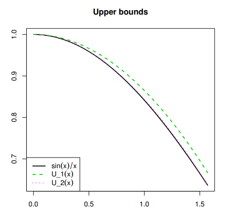
Obviously, the lower bound of \((\sin x)/x\) in (3) is refined in (7). Now suppose \[U_1(x) = 1 – \frac{4x^2}{3\pi^2} \, \, \, \text{and} \, \, \, U_2(x) = \left(1-\frac{x^2}{6}\right) + \left(\frac{\pi^2}{24}+\frac{2}{\pi}-1\right)(1-\cos x)^2.\]
Then we claim the following:
Proposition 1. For \(x \in (0, \pi/2),\) it holds that \[U_1(x) – U_2(x) > 0, \, \, \, \text{i.e.,} \, \, \, U_1(x) > U_2(x).\]
Proof. We need to prove that \[1 – \frac{4x^2}{3\pi^2} > \left(1-\frac{x^2}{6}\right) + \left(\frac{\pi^2}{24}+\frac{2}{\pi}-1\right)(1-\cos x)^2,\] i.e., \[\frac{x^2}{6} – \frac{4x^2}{3\pi^2} > \left(\frac{\pi^2}{24} + \frac{2}{\pi} – 1\right)(1-\cos x)^2 ,\] or \[\left( \frac{1}{6} – \frac{4}{3\pi^2} \right)x^2 > \left(\frac{\pi^2}{24} + \frac{2}{\pi} – 1\right)(1-\cos x)^2.\]
To prove this, we use Kober’s inequality [29, 35] \[1 – \cos x < \frac{2x}{\pi}; \, \, \, x \in (0, \pi/2),\] to write \[\begin{aligned} \label{eqn*} \frac{(1 – \cos x)^2}{x^2} < \frac{4}{\pi^2}; \, \, \, x \in (0, \pi/2). \end{aligned} \tag{9}\]
From the known relation \(\pi > 3,\) we have \(\frac{8}{\pi} < \frac{8}{3},\) i.e., \(\frac{8}{\pi} < 4 – \frac{4}{3}.\) This can be written as \[\frac{\pi^2}{6} + \frac{8}{\pi} – 4 < \frac{\pi^2}{6} – \frac{4}{3},\] i.e., \[4\left(\frac{\pi^2}{24} + \frac{2}{\pi} – 1 \right) < \pi^2 \left( \frac{1}{6} – \frac{4}{3\pi^2} \right),\] or \[\begin{aligned} \label{eqn**} \frac{4}{\pi^2} < \frac{\left( \frac{1}{6} – \frac{4}{3\pi^2} \right) }{\left(\frac{\pi^2}{24} + \frac{2}{\pi} – 1 \right)}. \end{aligned} \tag{10}\]
Combining (9) and (10), we get \[\frac{(1 – \cos x)^2}{x^2} < \frac{\left( \frac{1}{6} – \frac{4}{3\pi^2} \right) }{\left(\frac{\pi^2}{24} + \frac{2}{\pi} – 1 \right)},\] which is what we claimed. ◻
The following Figure 1 also supports our claim and shows that the upper bound of \((\sin x)/x\) in (7) is also sharper than the corresponding upper bound in (3). The curves \((\sin x)/x\) and \(U_2(x)\) nearly coincide.
Moreover, in (8), we obtained the bounds of \((\sin x)/x\) in a wider range of values of \(x,\) i.e., in \((0, \pi).\)
In the next theorem, we use the functions \(\left( 1- \frac{2x^2}{3\pi^2}\right)\) and \((1-\cos x)\) to refine inequalities (3).
Theorem 2. The function \(\left[\frac{\sin x}{x} – \left(1-\frac{2x^2}{3\pi^2}\right)\right] \big/ (1-\cos x)\) is strictly increasing from \((0, \pi)\) onto \((\delta_1, \delta_2),\) where \(\delta_1 = 2\left(\frac{2}{3\pi^2}-\frac{1}{6}\right)\) and \(\delta_2 = -\frac{1}{6}.\) In particular,
If \(x \in (0, \pi/2),\) then the inequality \[\begin{aligned} \label{eqn3.3} \left(1-\frac{2x^2}{3\pi^2}\right) + \frac{1}{3}\left(\frac{4}{\pi^2} – 1 \right) (1-\cos x) < \frac{\sin x}{x} < \left(1-\frac{2x^2}{3\pi^2}\right) + \left(\frac{2}{\pi}-\frac{5}{6}\right)(1-\cos x) , \end{aligned} \tag{11}\] holds with the optimal constants \(\frac{1}{3}\left(\frac{4}{\pi^2} – 1 \right)\) and \(\left(\frac{2}{\pi}-\frac{5}{6}\right)\) respectively.
If \(x \in (0, \pi),\) then the inequality \[\begin{aligned} \label{eqn3.4} \left(1-\frac{2x^2}{3\pi^2}\right) + \frac{1}{3}\left(\frac{4}{\pi^2} – 1 \right) (1-\cos x) < \frac{\sin x}{x} < \left(1-\frac{2x^2}{3\pi^2}\right) -\frac{1}{6}(1-\cos x) , \end{aligned} \tag{12}\] holds with the optimal constants \(\frac{1}{3}\left(\frac{4}{\pi^2} – 1 \right)\) and \(-\frac{1}{6}\) respectively.
Proof. Suppose \[g(x) = \frac{\left[\frac{\sin x}{x} – \left(1-\frac{2x^2}{3\pi^2}\right)\right]}{(1 – \cos x)} = \frac{g_1(x)}{g_2(x)}; \, \, \, x \in (0, \pi),\] where \(g_1(x) = \frac{\sin x}{x} – \left(1-\frac{2x^2}{3\pi^2}\right)\) and \(g_2(x) = 1 – \cos x\) are such that \(\lim_{x \rightarrow 0^+} g_1(x) = 0\) and \(g_2(0) = 0.\) Differentiation yields \[g_1'(x) = \frac{x \cos x – \sin x}{x^2} + \frac{4x}{3\pi^2} \, \, \, \text{and} \, \, \, g_2'(x) = \sin x \neq 0 \, \, \, \text{in} \, \, \, (0, \pi).\]
Hence \[\frac{g_1'(x)}{g_2'(x)} = \frac{1}{x} \cot x – \frac{1}{x^2} + \frac{4}{3\pi^2} \frac{x}{\sin x}.\] Based on series expansions in (4) and (5), we write \[\frac{g_1'(x)}{g_2'(x)} = \frac{1}{x^2} – \sum\limits_{k=1}^\infty \frac{2^{2k}}{(2k)!} \vert B_{2k} \vert x^{2k-2} – \frac{1}{x^2} + \frac{4}{3\pi^2} + \frac{4}{3\pi^2} \sum\limits_{k=1}^\infty \frac{2(2^{2k-1}-1)}{(2k)!} \vert B_{2k} \vert x^{2k}.\]
After the rearrangement of terms, we equivalently get \[\begin{aligned} \frac{g_1'(x)}{g_2'(x)} &= \frac{4}{3\pi^2} + \frac{4}{3\pi^2} \sum\limits_{k=1}^\infty \frac{2(2^{2k-1}-1)}{(2k)!} \vert B_{2k} \vert x^{2k} – \sum\limits_{k=0}^\infty \frac{2^{2k+2}}{(2k+2)!} \vert B_{2k+2} \vert x^{2k} \\ &= \left(\frac{4}{3\pi^2} – \frac{1}{3}\right) + \sum\limits_{k=1}^\infty \left[ \frac{8}{3\pi^2} \frac{(2^{2k-1}-1)}{(2k)!} \vert B_{2k} \vert – \frac{2^{2k+2}}{(2k+2)!} \vert B_{2k+2} \vert \right] x^{2k}. \end{aligned}\]
Then \[\left(\frac{g_1'(x)}{g_2'(x)}\right)' = \sum\limits_{k=1}^\infty \frac{16k}{(2k)!} \left[ \frac{(2^{2k-1}-1)}{3\pi^2} \vert B_{2k} \vert – \frac{2^{2k-1}}{(2k+2)(2k+1)} \vert B_{2k+2} \vert \right] x^{2k-1}.\]
To this end, for the positivity of the terms of the above series, we need to prove that \[\frac{(2^{2k-1}-1)}{3\pi^2} \vert B_{2k} \vert > \frac{2^{2k-1}}{(2k+2)(2k+1)} \vert B_{2k+2} \vert,\]i.e., \[\begin{aligned} \label{eqn3.5} \frac{\vert B_{2k+2} \vert}{\vert B_{2k} \vert} < \frac{(2k+1)(2k+2)}{\pi^2} \frac{(2^{2k-1}-1)}{3 \cdot 2^{2k-1}}; \, \, \, k = 1, 2, 3, \cdots. \end{aligned} \tag{13}\]
By virtue of absolute Bernoulli numbers \(\vert B_2 \vert = 1/6\) and \(\vert B_4 \vert = 1/30,\) for \(k = 1\), the inequality (13) becomes \(\frac{1}{5} < \frac{2}{\pi^2},\) i.e., \(\pi^2 < 10\) which is true. Now it remains to prove (13) for \(k = 2, 3, 4, \cdots.\) Because of the right inequality of Lemma 3, the relation (13) will be proved for \(k = 2, 3, 4, \cdots\) if \[\frac{(2^{2k}-1)}{(2^{2k+2}-1)} \cdot \frac{(2k+1)(2k+2)}{\pi^2} < \frac{(2k+1)(2k+2)}{\pi^2} \cdot \frac{(2^{2k-1}-1)}{3 \cdot 2^{2k-1}}; \, \, \, k = 2, 3, 4, \cdots,\]i.e., \[\frac{2^{2k}-1}{2^{2k+2}-1} < \frac{2^{2k-1}-1}{3 \cdot 2^{2k-1}}; \, \, \, k = 2, 3, 4, \cdots,\]i.e., \[3 \cdot 2^{4k-1}- 3 \cdot 2^{2k-1} < 2^{4k+1} – 2^{2k-1} – 2^{2k+2} + 1,\] or \[2^{2k} + 2^{2k+3} < 2^{4k} + 3 \cdot 2^{2k} + 2,\] which is equivalent to \[3 \cdot 2^{2k+1} < 2^{4k} + 2,\] i.e., \[2^{2k}(2^{2k}-6) + 2 > 0.\]
The last relation holds as \(2^{2k}-6 > 0\) for \(k = 2, 3, 4, \cdots.\) Thus the derivative of \(g_1'(x)/g_2'(x)\) is positive, so it is strictly increasing in \((0, \pi).\) By Lemma 1, \(g(x)\) is also strictly increasing in \((0, \pi).\) As a result, for \(x \in (0, \pi/2),\) we have \[\frac{1}{3}\left(\frac{4}{\pi^2} – 1 \right) = \lim_{x \rightarrow 0^+} g(x) < g(x) < \lim_{x \rightarrow \pi/2^-} g(x) = \left(\frac{2}{\pi}-\frac{5}{6}\right).\]
This gives inequality (11). Similarly for \(x \in (0, \pi),\) we have \[\frac{1}{3}\left(\frac{4}{\pi^2} – 1 \right) = \lim_{x \rightarrow 0^+} g(x) < g(x) < \lim_{x \rightarrow \pi^-} g(x) = -\frac{1}{6}.\]
This gives inequality (12) and the proof of Theorem 2 is completed. ◻
It is clear that the upper bound of \((\sin x)/x\) in (11) is sharper than the corresponding upper bound in (2). Let us now compare the bounds of \((\sin x)/x\) in (3) and (11) graphically. We consider the difference functions \[l(x) = \left(1-\frac{2x^2}{3\pi^2}\right) + \frac{1}{3}\left(\frac{4}{\pi^2} – 1 \right) (1-\cos x) – \left(1 – \frac{x^2}{6}\right),\] and \[u(x) = \left(1-\frac{4x^2}{3\pi^2}\right) – \left(1-\frac{2x^2}{3\pi^2}\right) – \left(\frac{2}{\pi}-\frac{5}{6}\right)(1-\cos x).\]
The aforementioned difference functions are displayed in Figure 2.
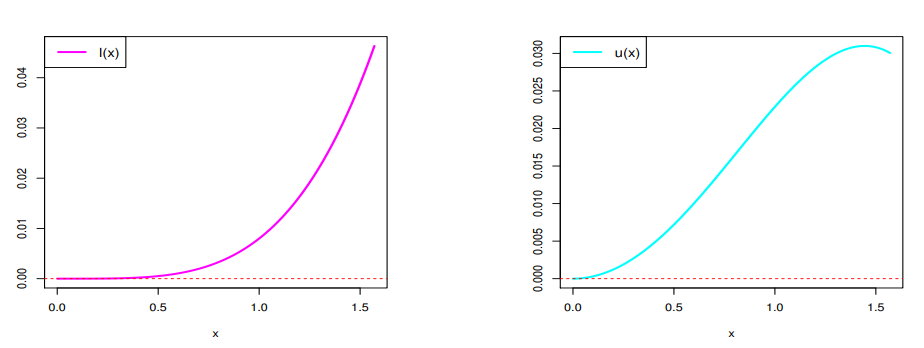
From Figure 2, one can confirm that the bounds of \((\sin x)/x\) in (11) are superior to those in (3) in terms of sharpness. This confirmation is proved in the following proposition.
Proposition 2. For \(x \in (0, \pi/2),\) it holds that \[l(x) > 0 \, \, \, \text{and} \, \, \, u(x) > 0.\]
Proof. First note that proving \(l(x) > 0\) is equivalent to prove that \[\left(\frac{1}{6} – \frac{2}{3\pi^2} \right)x^2 + \frac{1}{3}\left(\frac{4}{\pi^2}-1\right)(1-\cos x) > 0,\] i.e., \[\frac{1}{6}\left(1-\frac{4}{\pi^2}\right) x^2 > \frac{1}{3}\left(1-\frac{4}{\pi^2}\right)(1-\cos x),\] or \[\frac{1}{2} > \frac{(1-\cos x)}{x^2},\] which is true due to the inequality [29] \[1 – \frac{x^2}{2} < \cos x; \, \, \, x \in (0, \pi/2).\]
Similarly, proving \(u(x) > 0\) is equivalent to prove that \[-\frac{2x^2}{3\pi^2} – \left(\frac{2}{\pi} – \frac{5}{6}\right)(1 – \cos x) > 0,\] i.e., \[\left(\frac{5}{6} – \frac{2}{\pi}\right)(1-\cos x) > \frac{2x^2}{3\pi^2},\] or \[\frac{(1-\cos x)}{x^2} > \frac{4}{\pi(5 \pi -12)}.\]
Thanks to the Kober type inequality [29] \[\cos < 1 – \frac{4x^2}{\pi^2}; \, \, \, x \in (0, \pi/2),\] which can be also be written as \[\begin{aligned} \label{eqn@} \frac{(1-\cos x)}{x^2} > \frac{4}{\pi^2}; \, \, \, x \in (0, \pi/2). \end{aligned} \tag{14}\]
Now the relation \(\pi > 3\) allows us to write \(5\pi – 12 > \pi\) or \[\begin{aligned} \label{eqn@@} \frac{4}{\pi^2} > \frac{4}{\pi (5\pi – 12)}. \end{aligned} \tag{15}\]
From (14) and (15), we get the desired result. ◻
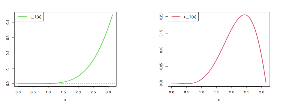
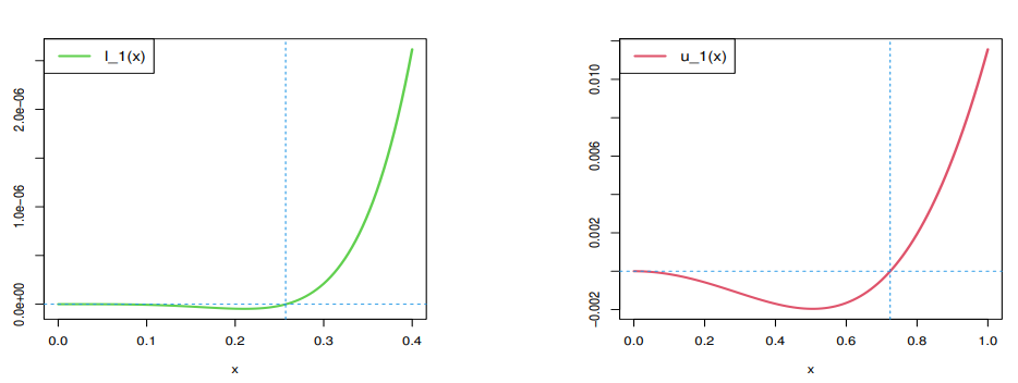
Lastly, it is natural to ask which bounds of \((\sin x)/x\) are better for \(x \in (0, \pi).\) Numerical observations and some graphical comparisons reveal the following:
There is no strict comparison between the corresponding bounds of \((\sin x)/x\) in (8) and (12).
The lower bound of \((\sin x)/x\) in (12) is sharper than that in (8) except in the interval \((0, \gamma),\) where \(\gamma \approx 0.257.\)
The upper bound of \((\sin x)/x\) in (12) is sharper than in (8) except in the interval \((0, \zeta),\) where \(\zeta \approx 0.724.\)
The above observations are visually confirmed by Figure 3 and Figure 4, where the curves of the difference functions \[l_1(x) = \left(1-\frac{2x^2}{3\pi^2}\right) + \frac{1}{3}\left(\frac{4}{\pi^2} – 1 \right) (1-\cos x) – \left(1-\frac{x^2}{6}\right) – \frac{1}{30}(1-\cos x)^2,\] and \[u_1(x) = \left(1-\frac{x^2}{6}\right) + \frac{1}{4} \left(\frac{\pi^2}{6}-1\right)(1-\cos x)^2 – \left(1-\frac{2x^2}{3\pi^2}\right) + \frac{1}{6}(1-\cos x) ,\] are plotted. Here the approximated values of \(\gamma\) and \(\zeta\) can be found by one of the root-finding methods such as Bisection method, Regula falsi method etc.
There are several standard methods to evaluate the integral of sinc function over the set of non-negative real numbers. The value of this so-called Dirichlet integral \(\int_0^\infty \frac{\sin x}{x} dx\) is \(\pi/2.\) On the other hand, the partial integral is naturally expressed in terms of the sine integral \(Si(r) = \int_0^r \frac{\sin x}{x} dx,\) for any \(r > 0,\) so simple elementary closed forms are unavailable; therefore explicit upper and lower bounds remain useful. In such a case, an alternative way is to approximate the concerned sinc integral. By using our main results, we can better approximate \(\int_0^r \frac{\sin x}{x} dx,\) where \(0 < r \leq \pi.\) We can integrate the double inequality (12), because it holds point-wise over \([0, r].\) In particular, we have the following: \[I_1 = \frac{(11\pi + 12)}{36} + \frac{(2\pi – 4)}{3\pi^2} < \int_0^{\pi/2} \frac{\sin x}{x} dx < \frac{(7\pi+3)}{18} = I_2,\] and \[I_3 = \frac{4\pi}{9} + \frac{4}{3\pi} < \int_0^\pi \frac{\sin x}{x} dx < \frac{33\pi}{54} = I_4.\]
Therefore, the sinc integrals can be approximated as: \[\int_0^{\pi/2} \frac{\sin x}{x} dx \approx \frac{I_1 + I_2}{2} \approx 1.379387,\] and \[\int_0^\pi \frac{\sin x}{x} dx \approx \frac{I_3 + I_4}{2} \approx 1.870269.\]
Thus our approximations are better estimates for sinc integral with small absolute error bounds \(0.009011\) and \(0.049593\) respectively, i.e., \[\Bigg\vert \int_0^{\pi/2} \frac{\sin x}{x} dx – \frac{I_1 + I_2}{2} \Bigg\vert \leq \frac{I_2 – I_1}{2} \approx 0.009011,\] and \[\Bigg\vert \int_0^{\pi} \frac{\sin x}{x} dx – \frac{I_3 + I_4}{2} \Bigg\vert \leq \frac{I_4 – I_3}{2} \approx 0.049593.\]
In this section, we generalize and reformulate the established inequalities using the concept of stratification, which has been introduced recently, see for instance [18, 19, 21, 36– 39].
Let \(\left\lbrace \varphi_p(x) \right\rbrace_{p \in \mathbb{P}}\) be a family of functions that we consider for values of the argument \(x \in \mathbb{S} \subseteq \mathbb{R}\) and values of the parameter \(p \in \mathbb{P} \subseteq \mathbb{R}.\) The family of functions \(\left\lbrace \varphi_p(x) \right\rbrace_{p \in \mathbb{P}}\) is increasingly stratified on the set \(\mathbb{S}\) with respect to the parameter \(p \in \mathbb{P}\) if \[p_1 < p_2 \Longleftrightarrow \varphi_{p_1}(x) < \varphi_{p_2}(x); \, \, \, \forall x \in \mathbb{S} \, \, \, \text{and} \, \, \, \forall p_1, p_2 \in \mathbb{P}.\]
Similarly, The family of functions \(\left\lbrace \varphi_p(x) \right\rbrace_{p \in \mathbb{P}}\) is decreasingly stratified on the set \(\mathbb{S}\) with respect to the parameter \(p \in \mathbb{P}\) if \[p_1 < p_2 \Longleftrightarrow \varphi_{p_1}(x) > \varphi_{p_2}(x); \, \, \, \forall x \in \mathbb{S} \, \, \, \text{and} \, \, \, \forall p_1, p_2 \in \mathbb{P}.\]
Based on the inequalities from Theorem 1, we can introduce the family of functions \(\left\lbrace \varphi_p(x) \right\rbrace_{p \in \mathbb{P}},\) where \[\varphi_p(x) = \frac{\sin x}{x} – \left(1-\frac{x^2}{6}\right) – p(1-\cos x)^2,\] for \(x \in (0, \pi)\) and \(p \in \mathbb{P} = \mathbb{R}.\) It holds that \[\frac{\partial \varphi_p(x)}{\partial p} = – (1-\cos x)^2 < 0,\] for \(x \in (0, \pi).\) Therefore, the family of functions \(\left\lbrace \varphi_p(x) \right\rbrace_{p \in \mathbb{P}}\) is decreasingly stratified on the interval \((0, \pi)\) with respect to the parameter \(p \in \mathbb{P} = \mathbb{R}.\)
Since we proved in Theorem 1 that \(\varphi_p(x) > 0\) for \(x \in (0, \pi/2)\) and \(p = 1/30,\) from the definition of decreasingly stratified families of functions, it directly follows that \(\varphi_p(x) > 0\) for \(x \in (0, \pi/2)\) and \(p \leq 1/30.\)
Similarly, since \(\varphi_p(x) < 0\) for \(x \in (0, \pi/2)\) and \(p = \pi^2/24 + 2/\pi -1,\) from the definition of decreasingly stratified families of functions, it directly follows that \(\varphi_p(x) < 0\) for \(x \in (0, \pi/2)\) and \(p \geq \pi^2/24 + 2/\pi -1.\) Let \[A = \frac{1}{30} \, \, \, \text{and} \, \, \, B = \frac{\pi^2}{24} + \frac{2}{\pi} – 1.\]
The case when \(p \in ( A, B)\) and \(x \in (0, \pi/2)\) could also be considered using the parametric method from [38]. The parametric method for proving some analytic inequalities from [38] is based on the analysis of the function \(f : \mathbb{S} \longrightarrow \mathbb{P}\) such that \[f(x) = p \Longleftrightarrow \varphi_p(x) = 0,\] if such a function exists. In [38], based on the monotonicity of the function \(f\), the sign of the functions \(\varphi_p(x)\) is determined. Theorem 5 from [38] is stated as:
Theorem 3. ([38, Theorem 5]) Let \(\left\lbrace \varphi_p(x) \right\rbrace_{p \in \mathbb{P}}\) be a family of functions for \(x \in \mathbb{S} = (a, b) \subseteq \mathbb{R}\) and let \(\mathbb{P} \subseteq \mathbb{R} \, (\mathbb{P} \neq \emptyset),\) satisfying the following conditions:
1. the family of functions \(\left\lbrace \varphi_p(x) \right\rbrace_{p \in \mathbb{P}}\) is increasingly (decreasingly) stratified on the interval \((a, b);\)
2. there exists a continuous monotonically increasing function \(g : (a, b) \longrightarrow \mathbb{P}\) that satisfies \(g(x) = p \Longleftrightarrow \varphi_p(x) = 0\);
3. there exist limits \(\lim_{x \rightarrow a} g(x) = A\) and \(\lim_{x \rightarrow b} g(x) = B\) in \(\mathbb{\bar{R}}\) such that \((A, B) \subseteq \mathbb{P}.\)
Then, it holds:
(i) If \(p \leq A,\) then \[(\forall x \in (a, b)) \, \, \varphi_p(x) \leq \varphi_A(x) < 0 \, \, \, \, ((\forall x \in (a, b)) \, \varphi_p(x) \geq \varphi_A(x) > 0).\]
(ii) If \(p \in (A, B),\) then the equality \(\varphi_p(x) = 0\) has a unique solution \(x_0^{(p)} \in (a, b)\) and it holds that \[\left(\forall x \in \left(a, x_0^{(p)}\right) \right) \, \varphi_p(x) > 0 \, \, \, \, \left( \left(\forall x \in \left(a, x_0^{(p)}\right) \right) \, \varphi_p(x) < 0\right),\] and \[\left(\forall x \in \left( x_0^{(p)}, b\right) \right) \, \varphi_p(x) < 0 \, \, \, \, \left( \left(\forall x \in \left(x_0^{(p)}, b\right) \right) \, \varphi_p(x) > 0\right).\]
(iii) If \(p \geq B,\) then \[(\forall x \in (a, b)) \, \, \varphi_p(x) \geq \varphi_B(x) > 0 \, \, \, \, ((\forall x \in (a, b)) \, \varphi_p(x) \leq \varphi_B(x) < 0).\]
Now in Theorem 1, it holds that \[\varphi_p(x) = 0 \Longleftrightarrow f(x) = p = \frac{\frac{\sin x}{x}-\left(1-\frac{x^2}{6}\right)}{(1-\cos x)^2}.\]
We already proved that the function \(f\) is increasing for \(x \in (0, \pi)\) and obtained the values \(\lim_{x\rightarrow 0+} f(x) = A\) and \(f(\pi/2) = B.\) Hence all conditions for the application of Theorem 3 are satisfied, from which we deduce the following:
(i) If \(p \in (-\infty, A),\) it holds that \[\frac{\sin x}{x} > \left(1-\frac{x^2}{6}\right) + A(1-\cos x)^2 > \left(1-\frac{x^2}{6}\right) + p(1-\cos x)^2; \, \, \, x \in (0, \pi/2),\] and the constant \(A\) is the best possible.
(ii) If \(p \in (A, B),\) the equation \(\varphi_p(x) = 0\) has a unique solution \(x_0^{(p)}\) and it holds that \[\frac{\sin x}{x} < \left(1-\frac{x^2}{6}\right) + p(1-\cos x)^2; \, \, \, x \in \left(0, x_0^{(p)}\right),\] and \[\frac{\sin x}{x} > \left(1-\frac{x^2}{6}\right) + p(1-\cos x)^2; \, \, \, x \in \left(x_0^{(p)}, \frac{\pi}{2}\right).\]
(iii) If \(p \in (B, +\infty),\) it holds that \[\frac{\sin x}{x} < \left(1-\frac{x^2}{6}\right) + B(1-\cos x)^2 < \left(1-\frac{x^2}{6}\right) + p(1-\cos x)^2; \, \, \, x \in (0, \pi/2),\] and the constant \(B\) is the best possible.
We have also obtained that \[\lim_{x \rightarrow \pi-} f(x) = \frac{1}{4}\left(\frac{\pi^2}{6} – 1\right) := C.\]
Moreover, the function \(f\) is increasing for \(x \in (0, \pi),\) we can also apply Theorem \(5\) from [38] for \(x \in (0, \pi),\) from which we obtain:
(iv) If \(p \in (-\infty, A),\) it holds that \[\frac{\sin x}{x} > \left(1-\frac{x^2}{6}\right) + A(1-\cos x)^2 > \left(1-\frac{x^2}{6}\right) + p(1-\cos x)^2; \, \, \, x \in (0, \pi),\] and the constant \(A\) is the best possible.
(v) If \(p \in (A, C),\) the equation \(\varphi_p(x) = 0\) has a unique solution \(x_0^{(p)}\) and it holds that \[\frac{\sin x}{x} < \left(1-\frac{x^2}{6}\right) + p(1-\cos x)^2; \, \, \, x \in \left(0, x_0^{(p)}\right),\] and \[\frac{\sin x}{x} > \left(1-\frac{x^2}{6}\right) + p(1-\cos x)^2; \, \, \, x \in \left( x_0^{(p)}, \pi \right).\]
(vi) If \(p \in (C, +\infty),\) it holds that \[\frac{\sin x}{x} < \left(1-\frac{x^2}{6}\right) + C(1-\cos x)^2 < \left(1-\frac{x^2}{6}\right) + p(1-\cos x)^2; \, \, \, x \in (0, \pi),\] and the constant \(C\) is the best possible.
The inequalities in Theorem 2 can also be generalized completely analogously to the previous analysis using the parametric method. Here we have generalized them in \((0, \pi)\) only.
Let \[A_1 = \frac{1}{3}\left(\frac{4}{\pi^2} – 1\right), \, \, \, \text{and} \, \, \, C_1 = -\frac{1}{6}.\]
Then we obtain the following:
(a) If \(p \in (-\infty, A_1),\) it holds that \[\frac{\sin x}{x} > \left(1-\frac{2x^2}{3\pi^2}\right) + A_1(1-\cos x) > \left(1-\frac{2x^2}{3\pi^2}\right) + p(1-\cos x); \, \, \, x \in (0, \pi),\] and the constant \(A_1\) is the best possible.
(b) If \(p \in (A_1, C_1),\) the equation \(\frac{\sin x}{x} – \left( 1 – \frac{2x^2}{3\pi^2}\right) – p(1 – \cos x) = 0\) has a unique solution \(x_0^{(p)}\) and it holds that \[\frac{\sin x}{x} < \left(1-\frac{2x^2}{3\pi^2}\right) + p(1-\cos x); \, \, \, x \in \left(0, x_0^{(p)}\right),\] and \[\frac{\sin x}{x} > \left(1-\frac{2x^2}{3\pi^2}\right) + p(1-\cos x); \, \, \, x \in \left( x_0^{(p)}, \pi \right).\]
(c) If \(p \in (C_1, +\infty),\) it holds that \[\frac{\sin x}{x} < \left(1-\frac{2x^2}{3\pi^2}\right) + C_1(1-\cos x) < \left(1-\frac{2x^2}{3\pi^2}\right) + p(1-\cos x); \, \, \, x \in (0, \pi),\] and the constant \(C_1\) is the best possible.
The authors would like to thank anonymous referee for his/her careful reading, constructive comments and valuable suggestions which helped to improve the manuscript.