
Statistical process control (SPC) charts whose parameters are estimated from historical data inherit the sampling variability of those estimates. The Shewhart \(\bar{X}\)-chart and \(S\)-chart remain the most widely deployed SPC tools [1,2], yet their standard normal-theory forms can use the sample standard deviation \(S\), whose finite-sample breakdown point \(1/n\) approaches zero as \(n\) increases [3,4]. A single outlying observation can inflate \(\hat\sigma=S\), widen the limits, and mask genuine process shifts, a phenomenon widely documented in the SPC literature [5,6].
Estimation uncertainty compounds the masking problem. Jensen et al. [7] showed that estimating chart parameters from \(m\) subgroups produces a random FAP whose deviation from the nominal 0.0027 can be substantial when \(m\) is small. Jones-Farmer et al. [8] and Psarakis et al. [9] review the literature on this parameter-estimation effect and recommend that charts with estimated limits explicitly account for estimation variability. The present paper commits to a single, precisely stated operating context throughout: parameters are estimated once from an independent Phase I reference sample, and the estimated limits are then applied prospectively to independent future subgroups (§2.1). We deliberately do not treat fully retrospective screening, in which the same historical subgroups are plotted against limits to whose estimation they contributed; that setting requires a different probability model (for example a leave-one-out or deletion formulation) and is identified in §5 as future work. This operating definition governs the terminology and interpretation used in the title, abstract, methods, simulations, applications, and conclusions throughout the present paper.
The median absolute deviation (MAD) achieves the maximum asymptotic breakdown point of 0.5 [10,4]. Abu-Shawiesh [11] derived MAD-based \(S\)-chart limits for known \(\sigma\), Adekeye and Azubuike [12] extended these to the \(\bar{X}\)-chart, and Adekeye [13] modified both sets of limits for the unknown-\(\sigma\) setting by substituting \(\hat\sigma=b_n\mathrm{MAD}\) into three-sigma limits, obtaining \(\mathrm{UCL}=\bar{\bar{X}}+A_6\overline{\mathrm{MAD}}\) with \(A_6=3b_n/\sqrt{n}\).
Despite this progress, several questions remain about estimation-adjusted MAD charts, and the present paper addresses them through the following theoretical and comparative analyses. First, the uncorrected multiplier \(A_6\) ignores the finite-\(m\) estimation variance of both the centre line and the pooled MAD; the finite-\(m\) FAP inflation that this causes has been demonstrated for classical charts [14] and motivates an explicit treatment of the MAD estimator in the present setting; §2.5 derives the correction from the exact unconditional FAP. Second, the present study provides a systematic comparison at a common in-control FAP between MAD-based charts and the \(S_n\) and \(Q_n\) estimators of Rousseeuw and Croux [4] or the trimmed and Winsorized estimators reviewed by Wilcox [15]; uncalibrated performance comparisons do not isolate detection performance at a common false-alarm rate and are retained only as secondary evidence (§3.4). Third, robustness to distributional shape and robustness to contamination are distinct properties; a dedicated \(\varepsilon\)-contamination study is added (§3.6). Fourth, the two case studies are presented as what they are: fully documented synthetic benchmark datasets for which the reported values are computed from the observations printed in the appendix (§3.7–§3.8).
Applications of SPC tools in Nigerian manufacturing and process industries further motivate this work. Ayenigba [16] applies control charts and process-capability indices to dimensional consistency in soap manufacturing. Ayenigba and Ajao [17] examine statistical quality control in sachet-water production and marketing. These studies provide application context; they do not establish that all such processes are non-normal or validate the MAD correction developed here. The term parameter-estimation-adjusted is used because the chart multiplier is fixed at the design stage from the known Phase I sample size \(m\) and is not updated in response to incoming observations. In contrast, Capizzi and Masarotto [18] develop an adaptive EWMA chart whose weighting responds to the current error. Alaeddini et al. [19] address the related but distinct task of estimating change points in fixed and variable sampling charts.
Throughout this paper the operating context is the following. Let \(X_{ij}\), \(i=1,\dots,n\), \(j=1,\dots,m\), be independent observations from a continuous in-control distribution \(F\) with location \(\mu_0\) and finite standard deviation \(\sigma_0>0\). These \(mn\) observations constitute the Phase I reference dataset from which the centre line and control limits are estimated. The estimated limits \([\hat L,\hat U]\) are then applied prospectively to future subgroups of size \(n\) drawn independently from the same \(F\). Writing \(\bar X_{\mathrm{new}}\) for the mean of one such future subgroup, the unconditional false alarm probability is
where \(\hat\theta=(\bar{\bar{X}},\hat\sigma)\) collects the Phase I estimates and the outer expectation in (1) is taken over the joint distribution of \((\bar{\bar{X}},\hat\sigma)\). This is the setting usually described as Phase II monitoring with estimated parameters [7,8]; we refer to it simply as prospective monitoring with estimated limits. Fully retrospective screening of the same \(m\) subgroups used to compute the limits requires a different probability model and is not treated here. All simulations, run-length evaluations, and benchmark analyses in this paper conform to definition (1).
Let \(\bar X_j=n^{-1}\sum\limits_{i=1}^n X_{ij}\) and \(\bar{\bar{X}}=m^{-1}\sum\limits_{j=1}^m\bar X_j\). Throughout, \(\sigma_0\) denotes the ordinary in-control standard deviation of \(F\). All scale estimators below are normalised with normal-reference constants: each population-defined normalisation is exactly unbiased for \(\sigma_0\) at the stated \(n\) when \(F=N(\mu_0,\sigma_0^2)\). Outside the normal family the six estimators generally converge to different functionals of \(F\), none of which need equal \(\sigma_0\). Two consequences follow and are drawn explicitly. (i) A narrower control-limit interval under a non-normal \(F\) cannot by itself be interpreted as greater efficiency, because it may reflect downward bias of the underlying scale functional relative to \(\sigma_0\); interval-width comparisons are therefore made only under normality or after calibration. (ii) All out-of-control comparisons in §3.4 are performed only after each chart has been calibrated, per distribution, subgroup size, and estimator, to the common unconditional in-control FAP of 0.0027, so that a common operating characteristic is enforced under every \(F\) studied.
For subgroup \(j\) let \(X_{(1)j}\le\dots\le X_{(n)j}\) denote the ordered observations. The six per-subgroup statistics are:
where \(\mathrm{SD}(\cdot)\) is the sample standard deviation with divisor equal to the number of retained values minus one. Two corrections are made to the trimmed and Winsorized estimators. First, the trimming proportion is set to \(\alpha=0.20\) rather than \(\alpha=0.10\): with \(n=5\) and \(\alpha=0.10\) one has \(g=\lfloor 0.5\rfloor=0\), so that nothing is trimmed or Winsorized and the nominal breakdown values would not apply. With \(\alpha=0.20\), \(g=1\) for \(n=5\) and \(g=2\) for \(n=10\), so one (respectively two) observations are removed or pulled in from each tail. Second, the asymptotic constant \((1-2\alpha)^{-1/2}\) often attached to the trimmed standard deviation is not exact in finite samples and is not used; instead, for every estimator a single finite-sample unbiasing constant is used,
estimated from \(4\times10^{6}\) independent \(N(0,1)\) subgroups (master seed 20260501) with Monte Carlo standard errors below \(6\times10^{-4}\); the constants are tabulated in Table 1, and it is these Monte Carlo values, not any exact closed-form alternative, that are used operationally throughout the paper for all six estimators, so that every chart’s unbiasing constant is obtained by the identical procedure.
| \(n\) | Estimator | \(E_{N(0,1)}[\text{raw}]\) | \(d_n\) | MC s.e.(\(d_n\)) |
|---|---|---|---|---|
| 5 | \(S\) | 0.9401 | 1.0638 | 1.9e-04 |
| 5 | MAD | 0.8221 | 1.2164 | 3.6e-04 |
| 5 | \(S_n\) | 0.7417 | 1.3483 | 3.7e-04 |
| 5 | \(Q_n\) | 1.1866 | 0.8427 | 2.3e-04 |
| 5 | Trim (\(\alpha{=}0.2\)) | 0.5200 | 1.9230 | 5.5e-04 |
| 5 | Win (\(\alpha{=}0.2\)) | 0.5103 | 1.9596 | 5.6e-04 |
| 10 | \(S\) | 0.9725 | 1.0283 | 1.2e-04 |
| 10 | MAD | 0.9122 | 1.0962 | 2.0e-04 |
| 10 | \(S_n\) | 0.9927 | 1.0074 | 1.7e-04 |
| 10 | \(Q_n\) | 1.3901 | 0.7194 | 1.1e-04 |
| 10 | Trim (\(\alpha{=}0.2\)) | 0.5080 | 1.9687 | 3.6e-04 |
| 10 | Win (\(\alpha{=}0.2\)) | 0.5826 | 1.7165 | 3.1e-04 |
For \(S\) alone an exact value, \(d_n(S)=1/C_4(n)\), happens to be available, and it is used solely as an independent unit test of the Monte Carlo machinery rather than as the operational constant: the test agrees closely at \(n=5\), where the Monte Carlo estimate matches the exact value to four decimals (\(1.0638\) against \(1.063846\)), and passes within ordinary sampling variation at \(n=10\) (\(1.0283\pm0.0001\) against the exact \(1.028109\), a difference of \(0.0002\), under two Monte Carlo standard errors). The small, immaterial gap between the \(n=10\) Monte Carlo and exact values for \(S\) is accordingly consistent with the stated Monte Carlo uncertainty: both the text and the code use the Monte Carlo constant of Table 1 for \(S\), exactly as for every other estimator. For the MAD, the constants \(d_5(\mathrm{MAD})=1.2164\) and \(d_{10}(\mathrm{MAD})=1.0962\) differ from the tabulated values \(b_5=1.206\) and \(b_{10}=1.087\) of [13] by less than one percent; the Monte Carlo values are used operationally throughout so that every constant in the paper traces to a single documented computation. The pooled scale estimate, unbiased under exact normal-reference normalisation, for any estimator is then
The pooling rule—average the \(m\) per-subgroup raw statistics, then apply \(d_n\) once—is stated here explicitly and used identically in the theory, the simulations, the benchmark analyses, and the released code.
With \(\hat\sigma_\bullet\) from (9), already unbiased for \(\sigma_0\) under normality, the chart limits are
where the width multiplier \(\lambda\) equals 1 for the classical uncorrected design, equals \(c^{*}(m,n)\) of (17) for the corrected MAD chart, and is determined numerically in the calibrated study of §3.4. No consistency constant appears outside \(\hat\sigma_\bullet\), so each constant enters exactly once. For the MAD chart with \(\lambda=1\) this reproduces \(\mathrm{UCL}^{(\mathrm{MAD})}=\bar{\bar{X}}+A_6\overline{\mathrm{MAD}}^{\dagger}\) with \(A_6=3\,d_n(\mathrm{MAD})/\sqrt{n}\) (where \(\overline{\mathrm{MAD}}^{\dagger}\) denotes the pooled raw MAD), giving \(A_6=1.6320\) for \(n=5\) and \(A_6=1.0400\) for \(n=10\); the classical \(S\)-based \(\bar X\)-chart is recovered with \(\hat\sigma_S=\bar S/C_4\) and \(A_3=3/(C_4\sqrt n)=1.4273\) for \(n=5\). Every chart studied in this paper, whichever of the six scale estimators it uses, is an \(\bar X\)-chart monitoring the subgroup mean under §2.1’s operating definition; “the \(S\)-based chart,” “the MAD-based chart,” and so on throughout the paper denote this \(\bar X\)-chart with \(\hat\sigma_\bullet\) substituted into (10), not a classical dispersion chart that plots the subgroup scale statistic itself and monitors it for shifts. Where the classical dispersion \(S\)-chart or \(\bar{X}\)-chart of [1,2] is meant instead, as in the Introduction, it is named in full.
Correct FAP Expression. Conditional on the Phase I estimates, the signal probability of the limits \(\hat U=\bar{\bar{X}}+H\), \(\hat L=\bar{\bar{X}}-H\) with half-width \(H=A_6^{*}\overline{\mathrm{MAD}}^{\dagger}\) is, for a normal in-control process,
and the design target is the unconditional FAP
with the expectation over the joint distribution of \((\bar{\bar{X}},\overline{\mathrm{MAD}}^{\dagger})\). This is the FAP of definition (1), since \(\bar{\bar{X}}\) enters the limits as well as the scale. The target is met to the order established in Proposition 1 and verified numerically in Table 2.
| Uncorrected (\(A_6\)) | Corrected (\(A_6^{*}\)) | |||||
|---|---|---|---|---|---|---|
| 2-4 \(m\) | FAP (s.e.) | MRL | \(D(370)\) | FAP (s.e.) | MRL | \(D(370)\) |
| 10 | 0.01073 (0.00006) | 151.9 | 0.6622 | 0.00301 (0.00002) | 1195.7 | 0.3285 |
| 15 | 0.00751 (0.00003) | 174.5 | 0.6576 | 0.00285 (0.00002) | 672.1 | 0.3901 |
| 20 | 0.00607 (0.00002) | 189.9 | 0.6533 | 0.00278 (0.00001) | 518.7 | 0.4291 |
| 25 | 0.00531 (0.00002) | 198.3 | 0.6525 | 0.00276 (0.00001) | 441.1 | 0.4598 |
| 30 | 0.00481 (0.00002) | 206.5 | 0.6495 | 0.00274 (0.00001) | 401.7 | 0.4800 |
| 50 | 0.00392 (0.00001) | 220.7 | 0.6484 | 0.00273 (0.00001) | 328.3 | 0.5334 |
| 100 | 0.00327 (0.00001) | 236.7 | 0.6422 | 0.00271 (0.00001) | 288.8 | 0.5779 |
Normalisation of the Scale-Estimation Variance. Let \(W=d_n(\mathrm{MAD})\,\overline{\mathrm{MAD}}^{\dagger}/\sigma_0\) be the unbiased pooled scale in \(\sigma_0\) units, so that \(E(W)=1\). Define
The finite-\(n\) values, estimated from the \(4\times10^{6}\) subgroups of Table 1, are \(\kappa_\tau^{2}=1.7075\) for \(n=5\) and \(\kappa_\tau^{2}=1.3640\) for \(n=10\). As \(n\to\infty\), \(d_n(\mathrm{MAD})\to1\), so \(\kappa_\tau^{2}=n\,\mathrm{Var}(\mathrm{MAD}_j)+o(1)\). Write \(\mathrm{MAD}_j=1.4826\,M_n\), where \(M_n\) is the sample median of \(|X_{ij}-\mathrm{med}_i(X_{ij})|\). For a distribution symmetric about its median, estimating the centre does not change the asymptotic variance of \(M_n\) [20], so \(M_n\) behaves as the median of \(n\) draws from \(|X|\), whose density at its median \(q_3=\Phi^{-1}(3/4)\) is \(2\varphi(q_3)\). The delta method gives \[n\,\mathrm{Var}(M_n)\;\to\;\frac{1}{4\{2\varphi(q_3)\}^{2}} =\frac{1}{16\,\varphi(q_3)^{2}},\] and, using the exact normal-consistency factor \(1/q_3\), conventionally rounded to \(1.4826\),
which corresponds to the 36.7% Gaussian efficiency of the MAD [4,20]. For non-normal processes \(\kappa_\tau^{2}\) is estimated empirically (§4).
Derivation of \(A_6^{*}\). Take \(\mu_0=0\) and \(\sigma_0=1\) without loss of generality, and write \[U=\sqrt n\,\bar{\bar{X}}\sim N\Bigl(0,\frac1m\Bigr),\qquad W=1+\Delta,\qquad E(\Delta)=0,\qquad \mathrm{Var}(\Delta)=\frac{\kappa_\tau^{2}}{mn}.\]
With \(A_6^{*}=c\,A_6\) the standardised half-width is \(3cW\), and (11) becomes \[p(U,\Delta)=1-\Phi\bigl(U+3cW\bigr)+\Phi\bigl(U-3cW\bigr).\]
Under assumption (R1), with \(\sigma_0\) fixed, \(\bar{\bar{X}}\) is a complete sufficient statistic for \(\mu_0\) based on all \(mn\) observations, whereas \(\mathrm{MAD}_j\) of (2) is translation-invariant and therefore ancillary. Basu’s theorem gives \[\bar{\bar{X}}\;\perp\;(\mathrm{MAD}_1,\dots,\mathrm{MAD}_m),\] exactly, and hence \(U\perp\Delta\). The sample median is translation-equivariant and so is not independent of \(\bar{\bar{X}}\); only \(\mathrm{MAD}_j\) is needed here.
Independence allows \(U\) to be integrated out before any expansion. For \(U\sim N(0,\tau^{2})\) and any constant \(k\), \[E_U\{\Phi(U+k)\}=\Phi\Bigl(\frac{k}{\sqrt{1+\tau^{2}}}\Bigr).\]
Taking \(\tau^{2}=1/m\) and \(k=\mp3cW\) gives \[E_U\{p(U,\Delta)\mid\Delta\}=g(W),\qquad g(w)=2\Bigl\{1-\Phi\Bigl(\frac{3cw}{\sqrt{1+1/m}}\Bigr)\Bigr\},\] so that \(E\{p\}=E\{g(W)\}\) exactly, with \(g\) a function of the single scalar \(W\). Put \(a_0=3c/\sqrt{1+1/m}\). Then \[g(1)=2\{1-\Phi(a_0)\},\qquad g'(1)=-2a_0\varphi(a_0),\qquad g”(1)=2a_0^{3}\varphi(a_0),\] and, since \(E(W-1)=0\) and \(\mathrm{Var}(W)=\kappa_\tau^{2}/(mn)\),
With \(a=3c\) we have \(a_0=a\{1-1/(2m)+O(m^{-2})\}\), which turns (15) into
Setting \(E\{p\}=2\{1-\Phi(3)\}\) and expanding \(\Phi\) about \(3\) gives \[c=1+\frac{1+9\kappa_\tau^{2}/n}{2m}+O(m^{-2}),\] which we write, with the exact location factor \(\sqrt{1+1/m}\) for the \(N(0,1/m)\) centre-line term, as
The two forms of \(c\) agree through the \(O(m^{-1})\) term. The multiplier exceeds \(A_6\), so the limits are widened. For \(n=5\) the values of \(c^{*}\) at \(m=10,15,20,25,30,50,100\) are \[1.2100,\ 1.1386,\ 1.1034,\ 1.0825,\ 1.0686,\ 1.0410,\ 1.0204.\]
Proposition 1. Assume (R1) \(X_{ij}\stackrel{iid}{\sim}N(\mu_0,\sigma_0^{2})\); (R2) the future subgroup is independent of the Phase I sample and drawn from the same distribution; (R3) \(n\ge 2\) fixed, \(m\to\infty\); (R4) the constants \(d_n(\mathrm{MAD})\) and \(\kappa_\tau^{2}\) of (8) and (13) are used. Then the chart with half-width \(A_6^{*}\overline{\mathrm{MAD}}^{\dagger}\) and \(A_6^{*}\) from (17) satisfies \[\mathrm{FAP}^{*}(m,n)=0.0027+O(m^{-2}).\]
Proof. By Basu’s theorem, \(U\perp\Delta\) exactly under (R1)–(R2), so \[E\{p(U,\Delta)\}=E\{g(W)\},\qquad g(w)=2\Bigl\{1-\Phi\Bigl(\frac{3cw}{\sqrt{1+1/m}}\Bigr)\Bigr\}.\]
The statistic \(W\) is the mean of \(m\) i.i.d. terms with moments of every order under normality, and \[E(W)=1,\qquad \mathrm{Var}(W)=\frac{\kappa_\tau^{2}}{mn},\qquad E(W-1)^{3}=O(m^{-2}),\qquad E(W-1)^{4}=O(m^{-2}).\]
The function \(g\) is a composition of \(\Phi\) with a linear map, so its derivatives of every order are bounded on \((0,\infty)\). A fourth-order Taylor expansion about \(w=1\) with Lagrange remainder gives \[\begin{aligned} E\{g(W)\}&=g(1)+\tfrac12\,g”(1)\,\mathrm{Var}(W) +\tfrac16\,g”'(1)\,E(W-1)^{3}+R,\\ |R|&\le\frac{\|g^{(4)}\|_\infty}{24}\,E(W-1)^{4}, \end{aligned}\] where the first-order term vanishes because \(E(W-1)=0\). The third-order term and \(R\) are \(O(m^{-2})\), which is (15). No cross term arises, since \(U\) has already been removed. Re-expressing (15) through \(a=3c\) as in (16) and setting \(E\{p\}=2\{1-\Phi(3)\}\) yields \(c=c^{*}(m,n)+O(m^{-2})\) with \(c^{*}\) of (17). At \(c=c^{*}\) the \(O(m^{-1})\) term of (16) vanishes, so that \(\mathrm{FAP}^{*}(m,n)=0.0027+O(m^{-2}).\) \(\square\)
Remark 1.Under skewed \(F\), \(\mathrm{Cov}(\bar{\bar{X}},\mathrm{MAD}_j)\neq0\) in general and the constants target different functionals (§2.2); the closed form (17) is then only a normal-theory approximation, and the numerically calibrated multiplier \(\hat\lambda\) of §3.4 is the recommended design. The correction targets the unconditional FAP of (1); practitioners requiring a conditional (per-realisation) performance guarantee should consider bootstrap adjustment, such as the method of Gandy and Kvaløy [21], with its assumptions and probability guarantee stated explicitly.
What the Correction Adds, and What Accuracy It Attains. The parameter-estimation literature establishes the importance of accounting for estimation variability when designing chart limits. Jensen et al. [7] review its effects on control-chart properties. Saleh et al. [14] examine the variability of EWMA performance with estimated parameters, while Zwetsloot et al. [22] develop robust Phase I dispersion estimation and evaluate its effect on subsequent EWMA monitoring. These studies motivate the present adjustment, whose precise unconditional-FAP expansion is derived above for the specified MAD-based chart. Two ingredients of (17) belong to that general programme and are not new here: the exact location factor \(\sqrt{1+1/m}\), which uses only \(\bar{\bar{X}}\sim N(\mu_0,\sigma_0^{2}/m)\) exactly under (R1)–(R2), and the third-order Taylor-expansion method, which produces a first-order-in-\(1/m\) correction for any chart whose scale estimate is asymptotically normal with a known relative variance. The MAD-based derivation combines the following three ingredients: \(\kappa_\tau^{2}= n\,\mathrm{Var}\{d_n(\mathrm{MAD})\,\mathrm{MAD}_j\}/\sigma_0^{2}\) itself, a quantity particular to the per-subgroup MAD statistic, verified by Monte Carlo (Table 1) and connected in closed form to its normal-reference \(n\to\infty\) limit \(1/(16q_3^{2}\varphi(q_3)^{2})\approx1.3605\) of (14); the demonstration, by Basu’s theorem, that the centre line and MAD are exactly, not merely asymptotically, independent under normality, a property shared by translation-invariant scale statistics under this normal model and one that removes any location–scale covariance term from the expansion without requiring an additional approximation; and the resulting closed-form multiplier \(A_6^{*}\) itself, which extends the previously available \(A_6\) limits of [13] from the unadjusted, setting without a finite-\(m\) estimation adjustment to the unconditional-FAP-calibrated one.
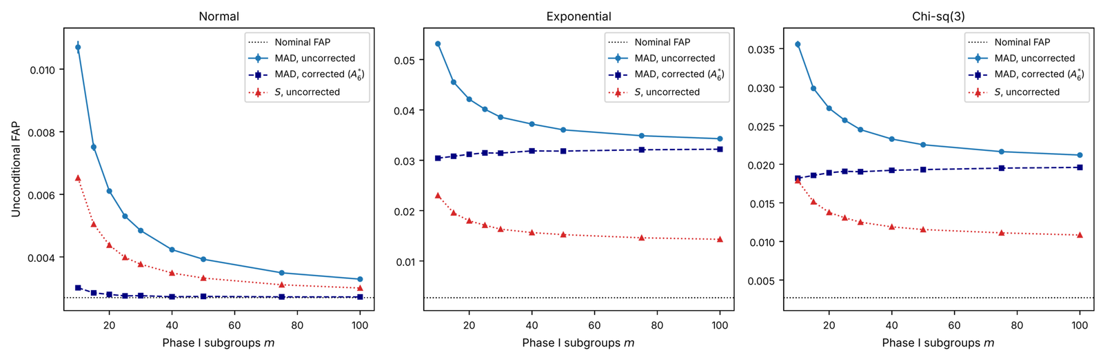
The accuracy of (17) against full numerical calibration is reported directly, not inferred. Table 2 compares the FAP delivered by \(A_6^{*}\) against the nominal 0.0027 under the Normal model, the model for which (17) is derived, across \(m\in\{10,\dots,100\}\) at \(n=5\), finding agreement within 6% of nominal for \(m\ge15\), consistent with the proven \(O(m^{-2})\) remainder of Proposition 1. This is a different exercise from Table 3, whose multiplier \(\hat\lambda\) is obtained by bisection to match the estimated target of 0.0027 to numerical precision under each of the four distributions studied there and so does not exercise the closed form at all; no claim in this paper infers the closed form’s accuracy under non-normal models from Table 3, and the Remark above states plainly that (17) is a normal-theory approximation requiring \(\hat\lambda\) once the reference distribution is appreciably skewed. The distributional information a practitioner must supply follows directly: (17) requires only that the Phase I data be approximately normal, in which case no further distributional knowledge beyond \(n\) and \(m\) is needed; outside that regime, the practitioner must either know the reference distribution well enough to calibrate \(\hat\lambda\) numerically (§3.4), in which case the additional uncertainty is the Monte Carlo error of that calibration (quantified for the Weibull model above), or accept the residual miscalibration documented in Figure 1 under the Exponential and \(\chi^2_3\) models, where no finite-\(m\) correction removes the asymptotic distributional bias and per-distribution calibration is the only remedy.
| Dist. | \(n\) | Est. | \(\hat\lambda\) | FAP\(_0\) (uncal.) | MRL\(_1(0.5)\) | MRL\(_1(1)\) | MRL\(_1(2)\) | MRL\(_1(-1)\) |
|---|---|---|---|---|---|---|---|---|
| Normal | 5 | \(S\) | 1.037 | 0.0038 | 28.91 | 3.26 | 0.28 | 3.24 |
| Normal | 5 | MAD | 1.069 | 0.0048 | 35.49 | 3.77 | 0.31 | 3.78 |
| Normal | 5 | \(S_n\) | 1.064 | 0.0046 | 34.62 | 3.70 | 0.30 | 3.70 |
| Normal | 5 | \(Q_n\) | 1.062 | 0.0046 | 33.95 | 3.65 | 0.30 | 3.64 |
| Normal | 5 | Trim (\(\alpha{=}0.2\)) | 1.070 | 0.0048 | 35.31 | 3.75 | 0.30 | 3.77 |
| Normal | 5 | Win (\(\alpha{=}0.2\)) | 1.069 | 0.0048 | 35.25 | 3.75 | 0.30 | 3.75 |
| Normal | 10 | \(S\) | 1.025 | 0.0034 | 9.83 | 0.91 | 0.09 | 0.91 |
| Normal | 10 | MAD | 1.038 | 0.0038 | 10.53 | 0.95 | 0.09 | 0.95 |
| Normal | 10 | \(S_n\) | 1.033 | 0.0037 | 10.25 | 0.93 | 0.09 | 0.93 |
| Normal | 10 | \(Q_n\) | 1.031 | 0.0036 | 10.07 | 0.92 | 0.09 | 0.92 |
| Normal | 10 | Trim (\(\alpha{=}0.2\)) | 1.037 | 0.0038 | 10.44 | 0.94 | 0.09 | 0.94 |
| Normal | 10 | Win (\(\alpha{=}0.2\)) | 1.038 | 0.0038 | 10.45 | 0.94 | 0.09 | 0.94 |
| Exponential | 5 | \(S\) | 1.456 | 0.0164 | 59.25 | 11.48 | 0.66 | 157.57 |
| Exponential | 5 | MAD | 1.895 | 0.0386 | 65.74 | 12.63 | 0.71 | 327.19 |
| Exponential | 5 | \(S_n\) | 1.927 | 0.0409 | 63.70 | 12.27 | 0.69 | 264.32 |
| Exponential | 5 | \(Q_n\) | 1.907 | 0.0396 | 63.86 | 12.30 | 0.70 | 260.30 |
| Exponential | 5 | Trim (\(\alpha{=}0.2\)) | 1.616 | 0.0233 | 65.22 | 12.54 | 0.71 | 323.78 |
| Exponential | 5 | Win (\(\alpha{=}0.2\)) | 1.621 | 0.0235 | 66.09 | 12.69 | 0.71 | 344.15 |
| Exponential | 10 | \(S\) | 1.282 | 0.0107 | 19.76 | 2.02 | 0.05 | 1.67 |
| Exponential | 10 | MAD | 1.698 | 0.0347 | 20.29 | 2.06 | 0.05 | 1.72 |
| Exponential | 10 | \(S_n\) | 1.733 | 0.0376 | 20.31 | 2.07 | 0.05 | 1.72 |
| Exponential | 10 | \(Q_n\) | 1.737 | 0.0380 | 19.95 | 2.03 | 0.05 | 1.68 |
| Exponential | 10 | Trim (\(\alpha{=}0.2\)) | 1.456 | 0.0187 | 20.32 | 2.07 | 0.05 | 1.72 |
| Exponential | 10 | Win (\(\alpha{=}0.2\)) | 1.457 | 0.0187 | 20.30 | 2.06 | 0.05 | 1.72 |
| Chi-sq(3) | 5 | \(S\) | 1.340 | 0.0125 | 49.33 | 8.73 | 0.51 | 23.49 |
| Chi-sq(3) | 5 | MAD | 1.595 | 0.0244 | 54.56 | 9.56 | 0.55 | 31.20 |
| Chi-sq(3) | 5 | \(S_n\) | 1.613 | 0.0256 | 53.27 | 9.35 | 0.54 | 29.22 |
| Chi-sq(3) | 5 | \(Q_n\) | 1.605 | 0.0251 | 53.07 | 9.32 | 0.54 | 28.99 |
| Chi-sq(3) | 5 | Trim (\(\alpha{=}0.2\)) | 1.441 | 0.0165 | 54.71 | 9.58 | 0.55 | 31.41 |
| Chi-sq(3) | 5 | Win (\(\alpha{=}0.2\)) | 1.446 | 0.0168 | 54.62 | 9.57 | 0.55 | 32.58 |
| Chi-sq(3) | 10 | \(S\) | 1.208 | 0.0083 | 16.48 | 1.64 | 0.06 | 1.37 |
| Chi-sq(3) | 10 | MAD | 1.441 | 0.0199 | 16.83 | 1.67 | 0.06 | 1.40 |
| Chi-sq(3) | 10 | \(S_n\) | 1.467 | 0.0216 | 16.77 | 1.67 | 0.06 | 1.40 |
| Chi-sq(3) | 10 | \(Q_n\) | 1.476 | 0.0223 | 16.49 | 1.64 | 0.06 | 1.38 |
| Chi-sq(3) | 10 | Trim (\(\alpha{=}0.2\)) | 1.313 | 0.0127 | 17.02 | 1.69 | 0.06 | 1.41 |
| Chi-sq(3) | 10 | Win (\(\alpha{=}0.2\)) | 1.318 | 0.0129 | 17.10 | 1.69 | 0.06 | 1.43 |
| Weibull(1.5) | 5 | \(S\) | 1.177 | 0.0075 | 35.04 | 5.41 | 0.36 | 6.50 |
| Weibull(1.5) | 5 | MAD | 1.289 | 0.0118 | 39.72 | 6.01 | 0.39 | 7.80 |
| Weibull(1.5) | 5 | \(S_n\) | 1.304 | 0.0126 | 39.16 | 5.94 | 0.39 | 7.67 |
| Weibull(1.5) | 5 | \(Q_n\) | 1.301 | 0.0125 | 38.78 | 5.89 | 0.38 | 7.62 |
| Weibull(1.5) | 5 | Trim (\(\alpha{=}0.2\)) | 1.211 | 0.0085 | 39.95 | 6.04 | 0.39 | 7.87 |
| Weibull(1.5) | 5 | Win (\(\alpha{=}0.2\)) | 1.214 | 0.0086 | 39.94 | 6.03 | 0.39 | 8.04 |
| Weibull(1.5) | 10 | \(S\) | 1.102 | 0.0053 | 11.97 | 1.19 | 0.07 | 1.05 |
| Weibull(1.5) | 10 | MAD | 1.181 | 0.0083 | 12.51 | 1.23 | 0.07 | 1.09 |
| Weibull(1.5) | 10 | \(S_n\) | 1.199 | 0.0091 | 12.43 | 1.23 | 0.07 | 1.08 |
| Weibull(1.5) | 10 | \(Q_n\) | 1.213 | 0.0098 | 12.17 | 1.21 | 0.07 | 1.06 |
| Weibull(1.5) | 10 | Trim (\(\alpha{=}0.2\)) | 1.122 | 0.0060 | 12.50 | 1.23 | 0.07 | 1.09 |
| Weibull(1.5) | 10 | Win (\(\alpha{=}0.2\)) | 1.124 | 0.0061 | 12.49 | 1.23 | 0.07 | 1.10 |
Two Distinct Estimands, and a Non-Existence Result. Conditional on the Phase I estimates \(\hat\theta\), the run length of a Shewhart chart with fixed estimated limits is geometric with parameter \(p_{\hat\theta}\), so its conditional mean is \(1/p_{\hat\theta}\). The unconditional false-alarm probability \(\mathrm{FAP}=E(p_{\hat\theta})\) is always well defined, since \(p_{\hat\theta}\in(0,1]\) is bounded. The unconditional mean run length \(\mathrm{ARL}=E(1/p_{\hat\theta})\) is not: a finite Monte Carlo average of \(1/p_{\hat\theta}\) across \(B\) replications is finite for every finite \(B\) regardless of whether the underlying expectation exists, so reporting such an average is not evidence of existence.
Proposition 2. Under (R1)–(R2) with \(m=10\), \(n=5\), and the corrected chart of Proposition 1, \(\mathrm{ARL}=E(1/p_{\hat\theta})=\infty\).
Proof. For \(t>0\) let \(A_t\) be the event that, in every subgroup, the five observations lie within distance \(1\) of the points \(-t,-t,0,t,t\) in some order. Four of the five observations per subgroup are then near \(\pm t\), so each subgroup has probability of order \(\varphi(t)^{4}\asymp e^{-2t^{2}}\), and over the ten independent subgroups \[\log\Pr(A_t)=-20\,t^{2}+O(t).\]
On \(A_t\) each subgroup median is \(O(1)\) and the absolute deviations are \(t+O(1),\,t+O(1),\,O(1),\,t+O(1),\,t+O(1)\), whose median is \(t+O(1)\). Hence \[\mathrm{MAD}_j=1.4826\,t+O(1),\qquad W=b\,t+O(1),\qquad b=1.2164\times1.4826=1.80343,\] while \(U=O(1)\), because each subgroup sum is \(O(1)\). With \(c^{*}(10,5)=1.2100\) the standardised half-width is \[a=3c^{*}W=3(1.2100)(1.80343)\,t+O(1)=6.547\,t+O(1).\]
By the Gaussian tail bound, \[p_{\hat\theta}\le2\{1-\Phi(a-|U|)\}\le\frac{2\varphi(a-|U|)}{a-|U|}.\]
Hence, on \(A_t\), \[\log\frac{1}{p_{\hat\theta}}\ge\frac{a^{2}}{2}+O(t)=21.43\,t^{2}+O(t).\]
Therefore \[\log E\Bigl(\frac{1}{p_{\hat\theta}}\Bigr) \ge\log\Pr(A_t)+\inf_{A_t}\log\frac{1}{p_{\hat\theta}} \ge1.43\,t^{2}+O(t)\;\longrightarrow\;\infty \quad(t\to\infty).\]
The left-hand side does not depend on \(t\), and hence \(E(1/p_{\hat\theta})=\infty\). \(\square\)
The mechanism is specific to small \(m\): widening the limits to compensate for a rare, extreme Phase I pooled-scale estimate makes the conditional run length on that realisation astronomically large, and the probability of the realisation does not decay fast enough to prevent this from dominating the mean. The result does not impugn the FAP calibration of Proposition 1, which targets a bounded quantity and is unaffected; it means only that the unconditional ARL is the wrong quantity to report alongside it. Two alternative summaries, computed from bounded survival probabilities, are used throughout the remainder of the paper. The continuously interpolated unconditional median run length \(\eta\) solves \(S(\eta)=1/2\) for the population survival function \(S(k)=E_{\hat\theta}\{(1-p_{\hat\theta})^{k}\}\), \(k=0,1,2,\dots\), which is bounded in \([0,1]\) for every real \(k\ge0\) and hence always well defined; because \(S(k)=E_{\hat\theta}\{\exp(k\log(1-p_{\hat\theta}))\}\) extends to non-integer \(k\) without approximation, \(\eta\) is located by bisection directly on this closed form rather than by interpolating a discrete grid. This continuous extension is the statistic denoted MRL in the tables; the median number of subgroups on the integer run-length scale is \(\lceil\eta\rceil\). The finite-horizon detection probability \(D(N)=E_{\hat\theta}\{1-(1-p_{\hat\theta})^{N}\}\) at a stated horizon \(N\) is likewise bounded in \([0,1]\) and answers the practically relevant question of how likely a signal is within a stated number of future subgroups. Neither estimand requires any run-length cap or censoring to remain finite, in contrast to \(E(1/p_{\hat\theta})\), which requires one to be well defined under simulation but is then not estimating the population quantity. At a sustained shift \(\delta\) the identical construction applied to \(p_{\hat\theta}(\delta)\) gives the out-of-control counterpart \(\mathrm{MRL}_1(\delta)\), which replaces \(\mathrm{ARL}_1(\delta)=E\{1/p_{\hat\theta}(\delta)\}\) in every comparison below. Whether contamination counts in §4 are fixed or independently resampled per replication is stated at each use; they are independently resampled, each of the \(mn\) Phase I observations replaced by an independent draw from the contaminating distribution with probability \(\varepsilon\), so the realised contamination count varies binomially about \(\varepsilon mn\) across replications rather than being held fixed.
Simulation Methodology and Precision. Every Monte Carlo experiment in this paper uses the following two-layer design. For each of \(B\) independent Phase I replications the estimates \((\bar{\bar{X}},\hat\sigma_\bullet)\) are computed and the conditional signal probability \(p_{\hat\theta}\) is then evaluated without a single Bernoulli alarm draw: under the Normal, Exponential, and \(\chi^2_3\) models the distribution of the subgroup mean is available in closed form (normal; shifted Gamma\((n)\); shifted, scaled \(\chi^2_{3n}\)), and under the Weibull model \(p_{\hat\theta}\) is evaluated against the empirical distribution of \(2\times10^{6}\) independently generated subgroup means. Unconditional FAP, median run length, and finite-horizon detection probability are then computed from the empirical distribution of \(p_{\hat\theta}\) across the \(B\) replications: FAP as the sample mean, with standard error \(\mathrm{sd}(p_{\hat\theta})/\sqrt B\); the median run length from the empirical survival function \(\hat S(k)=B^{-1}\sum\limits_b(1-p_{\hat\theta,b})^{k}\); and the detection probability as the sample mean of \(1-(1-p_{\hat\theta})^{N}\).
The Weibull empirical distribution deserves its own account. For each subgroup size \(n\in\{5,10\}\) a pool of \(M=2\times10^{6}\) independent subgroup means is generated once (seed \(777{,}000+n\)) and reused, without regeneration, for every one of the \(B\) Phase I replications and across every table and figure that reports a Weibull result, so that Monte Carlo noise in the reported quantities comes only from the \(B\) draws of \((\bar{\bar{X}},\hat\sigma_\bullet)\) against a single fixed reference distribution, not from resampling the pool itself. The conditional probability \(p_{\hat\theta}\) is evaluated against this pool as a plain empirical CDF, \(\hat F_n(x)=M^{-1}\sum\limits_{k=1}^{M} \mathbb{1}\{\bar W_k\le x\}\), located by binary search on the sorted pool with no smoothing or interpolation between pool points; beyond the pool’s most extreme value in either tail, \(\hat F_n\) saturates exactly at 0 or 1, so a control limit that falls beyond the most extreme of the \(2\times10^{6}\) simulated subgroup means would return an exact zero tail probability on that side for that replication (not encountered for any limit reported in this paper, since \(m=30\) and \(\lambda\approx1\) keep the limits well inside the pool’s range, but noted as the boundary behaviour of the method). Because the pool is itself a finite Monte Carlo object, it carries its own sampling error, distinct from the \(B\)-replication error already quantified above; this was checked directly by regenerating five further, independent \(M=2\times10^{6}\) pools (seeds \(888{,}000+n+1000k\), \(k=0,\dots,4\)) and recomputing, against each, the calibrated multiplier \(\hat\lambda\) and the uncalibrated in-control FAP for the \(S\)– and MAD-based charts at \(n=5\) with the \(B=20{,}000\) Phase I draw held fixed. Across the six independent pools (the production pool plus five replacements), \(\hat\lambda\) varies by a Monte Carlo standard deviation of \(0.0015\) (\(S\)) and \(0.0016\) (MAD) at \(n=5\), and \(0.0008\) and \(0.0008\) at \(n=10\) – below \(0.15\%\) relative to the reported values and immaterial at the precision quoted in Table 3; the uncalibrated FAP varies by a standard deviation of about \(4\times10^{-5}\) at \(n=5\) (roughly \(0.5\%\) relative to the reported \(0.0075\)–\(0.0118\)), while the calibrated FAP is, by the construction of the bisection search, insensitive to which pool is used, since each pool is recalibrated to the same 0.0027 target before any comparison is made. Pool sampling error is accordingly a minor contributor to the reported Weibull figures relative to the \(B\)-replication error already reported, and does not affect any qualitative conclusion of §3.4–3.6.
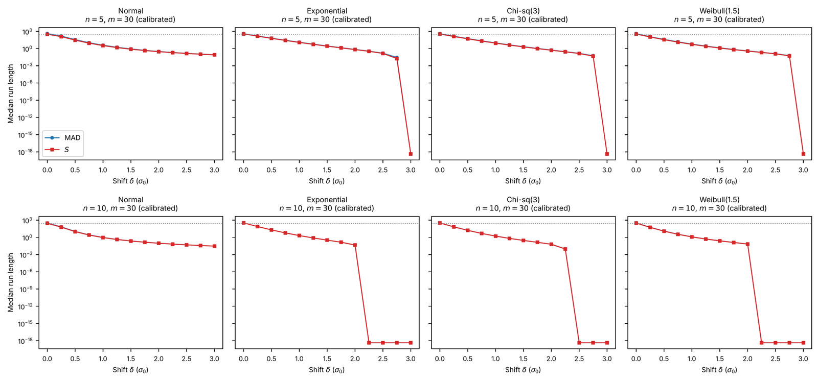
This exact-conditional-\(p\) design removes the Bernoulli noise floor entirely: a design in which each replication contributes a single 0/1 alarm indicator has standard error \(\{p(1-p)/B\}^{1/2}\approx0.0016\) at \(B=1{,}000\) and cannot distinguish 0.0027 from 0.0030. With the exact conditional-\(p\) design the FAP standard errors in Table 2 (\(B=100{,}000\)) are at most \(6\times10^{-5}\). Replication counts are uniform and documented: \(B=100{,}000\) for Table 2; \(B=30{,}000\) per point in Figure 1; \(B=20{,}000\) per cell in Tables 3 and 4; \(B=10{,}000\) per curve in Figure 2; \(B=5{,}000\) in Figure 3. Every seed is stated in the released code (Appendix A).
| \(H\) | \(\varepsilon\) | Est. | FAP\(_0\) | mean CLI | MRL\(_1(+1)\) | MRL\(_1(+2)\) | MRL\(_1(-1)\) |
|---|---|---|---|---|---|---|---|
| \(H=N(4,1)\) | 0.05 | \(S\) | 0.00050 | 3.511 | 38.69 | 0.89 | 6.03 |
| \(H=N(4,1)\) | 0.05 | MAD | 0.00191 | 3.230 | 18.53 | 0.64 | 3.51 |
| \(H=N(4,1)\) | 0.05 | \(S_n\) | 0.00163 | 3.263 | 20.00 | 0.66 | 3.74 |
| \(H=N(4,1)\) | 0.05 | \(Q_n\) | 0.00153 | 3.274 | 20.67 | 0.67 | 3.82 |
| \(H=N(4,1)\) | 0.05 | Trim (\(\alpha{=}0.2\)) | 0.00193 | 3.229 | 18.30 | 0.64 | 3.50 |
| \(H=N(4,1)\) | 0.05 | Win (\(\alpha{=}0.2\)) | 0.00193 | 3.226 | 18.07 | 0.64 | 3.49 |
| \(H=N(4,1)\) | 0.10 | \(S\) | 0.00020 | 4.143 | 1187.41 | 4.24 | 9.90 |
| \(H=N(4,1)\) | 0.10 | MAD | 0.00185 | 3.665 | 199.22 | 1.88 | 3.73 |
| \(H=N(4,1)\) | 0.10 | \(S_n\) | 0.00161 | 3.692 | 221.84 | 1.97 | 3.94 |
| \(H=N(4,1)\) | 0.10 | \(Q_n\) | 0.00149 | 3.705 | 235.60 | 2.02 | 4.02 |
| \(H=N(4,1)\) | 0.10 | Trim (\(\alpha{=}0.2\)) | 0.00136 | 3.776 | 281.67 | 2.21 | 4.56 |
| \(H=N(4,1)\) | 0.10 | Win (\(\alpha{=}0.2\)) | 0.00141 | 3.765 | 272.49 | 2.17 | 4.48 |
| \(H=N(0,9)\) | 0.05 | \(S\) | 0.00091 | 3.153 | 6.50 | 0.39 | 6.48 |
| \(H=N(0,9)\) | 0.05 | MAD | 0.00169 | 3.048 | 5.26 | 0.36 | 5.26 |
| \(H=N(0,9)\) | 0.05 | \(S_n\) | 0.00151 | 3.065 | 5.43 | 0.36 | 5.46 |
| \(H=N(0,9)\) | 0.05 | \(Q_n\) | 0.00147 | 3.075 | 5.57 | 0.37 | 5.52 |
| \(H=N(0,9)\) | 0.05 | Trim (\(\alpha{=}0.2\)) | 0.00180 | 3.021 | 4.99 | 0.35 | 5.01 |
| \(H=N(0,9)\) | 0.05 | Win (\(\alpha{=}0.2\)) | 0.00179 | 3.022 | 4.99 | 0.35 | 5.02 |
| \(H=N(0,9)\) | 0.10 | \(S\) | 0.00030 | 3.511 | 13.96 | 0.56 | 14.16 |
| \(H=N(0,9)\) | 0.10 | MAD | 0.00099 | 3.250 | 7.91 | 0.43 | 7.87 |
| \(H=N(0,9)\) | 0.10 | \(S_n\) | 0.00082 | 3.287 | 8.51 | 0.45 | 8.56 |
| \(H=N(0,9)\) | 0.10 | \(Q_n\) | 0.00077 | 3.306 | 8.92 | 0.46 | 8.85 |
| \(H=N(0,9)\) | 0.10 | Trim (\(\alpha{=}0.2\)) | 0.00108 | 3.206 | 7.17 | 0.41 | 7.20 |
| \(H=N(0,9)\) | 0.10 | Win (\(\alpha{=}0.2\)) | 0.00111 | 3.202 | 7.14 | 0.41 | 7.12 |
For a sustained mean shift \(\delta=(\mu_1-\mu_0)/\sigma_0\) imposed on the future subgroups only, \(p_{\hat\theta}(\delta)\) is obtained from the same closed forms with the subgroup-mean distribution translated by \(\delta\), and the out-of-control performance of the chart is summarised by the median run length \(\mathrm{MRL}_1(\delta)\) of §2.6, solving \(E_{\hat\theta}\{(1-p_{\hat\theta}(\delta))^{k}\}=1/2\) for \(k\), in place of the unconditional mean \(E\{1/p_{\hat\theta}(\delta)\}\), which Proposition 2 shows need not exist.
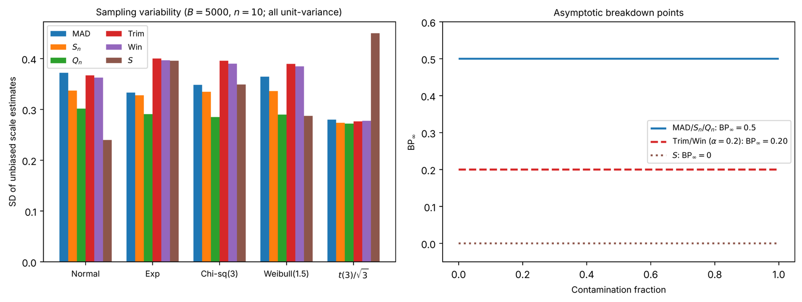
Table 1 reports the Monte Carlo finite-sample unbiasing constants \(d_n\) for all six estimators, together with their Monte Carlo standard errors, providing independently verified numerical values for all six estimators. The exact \(1/C_4(n)\) benchmark for \(S\) agrees to four decimals at \(n=5\) and within the stated Monte Carlo uncertainty at \(n=10\). Table 5 summarises breakdown and efficiency properties; asymptotic Gaussian efficiencies are quoted from [4] where an authoritative value exists, and finite-sample Gaussian relative efficiencies at \(n=5,10\), estimated from \(4\times10^{5}\) Monte Carlo subgroups, are reported for all six estimators. Because closed asymptotic ARE values for the trimmed and Winsorized standard deviations at \(\alpha=0.20\) are not available in a form matching definitions (6)–(7), no asymptotic value is asserted for them. Instead of reporting possibly convention-dependent finite-sample breakdown fractions, the table states the operationally meaningful quantity: the number of same-side outliers per subgroup of size 5 that each per-subgroup statistic tolerates (2 for MAD, \(S_n\), \(Q_n\); 1 for the \(\alpha=0.20\) trimmed and Winsorized statistics; 0 for \(S\)).
A qualification applies to every breakdown figure in this subsection and to the term high-breakdown used informally throughout the paper for the MAD-, \(S_n\)-, and \(Q_n\)-based charts. The asymptotic breakdown point of 0.5, and the two-same-side-outlier tolerance just stated, describe each per-subgroup statistic computed on its own \(n=5\) observations; neither transfers automatically to the chart actually used, whose scale estimate \(\hat\sigma_\bullet=d_n(\bullet)\,m^{-1}\sum\limits_j(\text{raw statistic})_j\) is an arithmetic average of \(m\) such subgroup values, nor to the centre line \(\bar{\bar{X}}\), the ordinary grand mean. A single arbitrarily extreme observation among the \(mn\) reference observations moves \(\bar{\bar{X}}\) without bound regardless of which scale estimator accompanies it, so the chart’s centre line has breakdown point 0 whatever \(\hat\sigma_\bullet\) is used; and three sufficiently separated extreme observations placed within one subgroup of five can make that subgroup’s MAD, \(S_n\), or \(Q_n\) arbitrarily large and hence make the arithmetically pooled \(\hat\sigma_\bullet\) arbitrarily large as well, even though only \(3/(mn)\) of the full reference sample is affected (2% at \(m=30\)). The \(\varepsilon\)-contamination study of §3.6 accordingly studies scattered contamination, independently distributed across all \(mn\) reference observations at a stated rate \(\varepsilon\le0.10\), not contamination concentrated within one or a few subgroups; its conclusions are restricted to that arrangement, and a chart’s resistance to it should not be read as evidence of a pooled breakdown point of 0.5.
| Tolerated outliers | Asymptotic | Finite-\(n\) Gaussian RE (%, MC) | |||
|---|---|---|---|---|---|
| Estimator | BP\(_\infty\) | per subgroup (\(n=5\)) | ARE (%) | \(n=5\) | \(n=10\) |
| \(S\) | 0 | 0 | 100 | 100.0 | 100.0 |
| MAD | 0.5 | 2 | 37 | 38.6 | 41.7 |
| \(S_n\) | 0.5 | 2 | 58 | 43.5 | 50.9 |
| \(Q_n\) | 0.5 | 2 | 82 | 45.5 | 63.3 |
| Trim (\(\alpha{=}0.2\)) | 0.2 | 1 | — | 40.0 | 43.0 |
| Win (\(\alpha{=}0.2\)) | 0.2 | 1 | — | 40.0 | 44.2 |
The in-control distributions, all standardised to mean 0 and variance 1, are: standard normal; standardised exponential \((X-1)\); standardised \(\chi^2_3\), \((X-3)/\sqrt6\); and standardised Weibull with shape \(k=1.5\), \((X-\mu_W)/s_W\) with the theoretical constants, shown here to six decimal places, \(\mu_W=\Gamma(1+1/k)\approx0.902745\) and \(s_W=\{\Gamma(1+2/k)-\mu_W^{2}\}^{1/2}\approx0.612936\). The \(t_3\) sample used in Figure 3 is likewise standardised to unit variance by dividing by \(\sqrt3\). Subgroup sizes are \(n\in\{5,10\}\) and the reference-sample size is \(m=30\) except where a grid over \(m\) is shown. All computations were run with Python 3, NumPy 2.4.4, SciPy 1.17.1, and Matplotlib 3.10.8; a single master script regenerates every table and figure from stored result objects, and the mapping from output objects to manuscript items, together with every seed, is listed in Appendix A.
Table 2 and Figure 1 quantify the FAP inflation of the uncorrected MAD chart and the effect of \(A_6^{*}\). At \(m=10\) the uncorrected FAP is \(0.01073\), four times nominal; the corrected chart attains \(0.00301\) at \(m=10\) and is within 6% of nominal (\(0.00285\)–\(0.00271\)) for all \(m\ge15\), consistent with the \(O(m^{-2})\) remainder of Proposition 1. The table also displays the interpolated median run length (MRL) and finite-horizon detection probability \(D(370)\) introduced in §2.6, in place of the unconditional mean \(E(1/p_{\hat\theta})\), which Proposition 2 shows is infinite at \(m=10\) for this chart and which is not reported for any \(m\) for that reason. The MRL is far above the naive geometric value \(\ln2/\mathrm{FAP}\approx230\) at \(m=10\) (1196) and falls toward it as \(m\) grows (289 at \(m=100\)), and \(D(370)\) – the probability of a signal within 370 subgroups, the conventional nominal in-control reference \(1/0.0027\) – rises from 0.33 to 0.58 over the same range: both reflect the same right-skewed mixing of \(p_{\hat\theta}\) across Phase I realisations that drives \(E(1/p_{\hat\theta})\) to infinity, without requiring that divergent quantity to be reported. This is consistent with the known heavy-tail behaviour of run lengths under estimated parameters [14] and is why the FAP, not the mean run length, is the design criterion here.
Every chart is therefore first calibrated: for each combination of distribution, \(n\), and estimator, the multiplier \(\hat\lambda\) in (10) is determined by bisection so that the unconditional in-control FAP equals 0.0027 exactly (to Monte Carlo accuracy) under that distribution, with \(m=30\) and \(B=20{,}000\) Phase I replications. Out-of-control performance is then compared at \(\delta\in\{0.5,1,2\}\) and, because the Exponential, \(\chi^2_3\), and Weibull models are asymmetric, also at negative shifts; Table 3 reports \(\mathrm{MRL}_1(-1)\) alongside the positive shifts. Uncalibrated in-control FAPs are retained as a secondary column, quantifying how far each normal-theory design departs from nominal under each distribution, but no superiority claim is based on them.
Three conclusions emerge, with each chart’s out-of-control performance reported as the always-defined \(\mathrm{MRL}_1(\delta)\) rather than a mean run length that Proposition 2 shows need not exist. First, under normality all six calibrated charts are nearly indistinguishable, the \(S\)-based chart being best by a small margin (\(\mathrm{MRL}_1(1)=3.26\) versus \(3.65\)–\(3.77\) for the robust charts at \(n=5\)), the familiar efficiency price of robustness. Second, under clean (uncontaminated) skewed data the calibrated \(S\)-based chart is competitive with, and for positive shifts somewhat better than, the robust charts (Exponential, \(n=5\): \(\mathrm{MRL}_1(1)=11.48\) for \(S\) against \(12.27\)–\(12.69\)); any apparent MAD superiority under skewness in uncalibrated comparisons rests entirely on unequal in-control ARLs. Third, detection of negative shifts under the skewed models is not uniformly fast for all charts: under the Exponential model, whose short left tail is reached quickly once the calibrated limits are widened, the MAD-family charts are roughly twice as slow as \(S\) at \(n=5\) (\(\mathrm{MRL}_1(-1)=327.2\) for MAD against \(157.6\) for \(S\); \(264.3\) and \(260.3\) for \(S_n\) and \(Q_n\); \(323.8\) and \(344.2\) for the trimmed and Winsorized charts), a gap traceable to the larger calibrated multiplier each robust estimator requires under skewness (\(\hat\lambda=1.895\) for MAD against \(1.456\) for \(S\) in Table 3); the gap narrows under \(\chi^2_3\) (\(31.2\) against \(23.5\)) and Weibull\((1.5)\) (\(7.80\) against \(6.50\)) and remains in \(S\)’s favour in these comparisons. This directional asymmetry is a genuine cost of robustness under clean skewed data, not an artefact of contamination, and negative-shift detection is therefore not unaffected by the choice of scale estimator. The genuine case for the high-breakdown estimators is made by the contamination study of §3.6, not by clean skewed data.
Figure 3 compares the sampling variability of the six unbiased estimators across five unit-variance distributions (the \(t_3\) panel is standardised by \(\sqrt3\) so that all five families are on the same scale) together with the asymptotic breakdown points, consistent with Table 5.
Robustness to distributional shape and robustness to contamination are different properties, and only the latter is what breakdown points describe. The Phase I reference sample is therefore contaminated according to
covering location outliers (assignable-cause observations that entered the reference data) and scale outliers (heavy-tailed measurement noise), with contaminated points scattered at random across subgroups. Each chart uses its normal-theory design calibrated at \(\varepsilon=0\) (the practitioner does not know contamination is present), and performance is evaluated against the clean in-control \(N(0,1)\): the in-control FAP measures masking of the false-alarm calibration, and \(\mathrm{MRL}_1\) at \(\delta=+1\), \(+2\), and \(-1\) measures the loss of detection power; \(n=5\), \(m=30\), \(B=20{,}000\) (Table 4).
The results give the breakdown-point discussion its empirical meaning. At \(\varepsilon=0.10\) with \(H=N(4,1)\) the \(S\)-based chart’s mean CLI inflates to \(4.14\) (clean value \(2.78\)), its calibration FAP collapses to \(0.00020\), one thirteenth of nominal, and its median run length at a subsequent \(+1\sigma\) shift lengthens to \(1187.4\) subgroups: the limits have been pulled so wide by the contaminated reference sample that the chart has effectively stopped detecting the shift. The high-breakdown estimators are affected far less: MAD’s calibration FAP falls only to \(0.00185\) and \(\mathrm{MRL}_1(+1)\) rises to \(199.2\), a sixfold improvement over \(S\); \(S_n\) and \(Q_n\) perform similarly (\(221.8\) and \(235.6\)). The \(\alpha=0.20\) trimmed and Winsorized charts, which tolerate only one outlier per subgroup of five rather than two, show the weakest masking resistance among the robust group (\(281.7\) and \(272.5\)) yet remain far closer to the MAD-family estimators than to \(S\), so that they do not degrade to \(S\)-like detection at this contamination level. Under \(\varepsilon=0.05\) the same ordering holds at smaller magnitudes (\(\mathrm{MRL}_1(+1)\): \(38.7\) for \(S\) against \(18.1\)–\(20.7\) for the five robust charts). Under scale contamination \(H=N(0,9)\) the masking is milder throughout: \(S\)’s FAP\(_0\) falls only to \(0.00030\) at \(\varepsilon=0.10\), and \(\mathrm{MRL}_1(+1)\) rises to \(14.0\) against \(7.1\)–\(8.9\) for the robust charts, because a symmetric variance inflation widens \(S\)’s own limits roughly in step with the shift it is trying to detect, unlike the asymmetric pull of a one-sided location contaminant. Together with §3.4, the evidence supports a precise conclusion: the high-breakdown charts are not superior under clean data of any shape studied here; they show substantially better positive-shift detection in the stated models with 5–10% scattered aberrant observations, which is precisely the situation Phase I estimation is exposed to in practice [8].
Both datasets are synthetic. They are generated from random-number generators with injected disturbances, and no real data collection, production records, or independently discovered assignable causes are claimed. The two generators were designed to emulate the statistical character of, respectively, sub-Saharan African urban PM\(_{2.5}\) series, which field measurements at several West African and neighbouring sites show to be right-skewed with episodic pollution spikes [23], and the Weibull-distributed tensile strength commonly used to model locally produced structural steel; the injected disturbances demonstrate detection and masking under known ground truth, which observed data cannot provide.
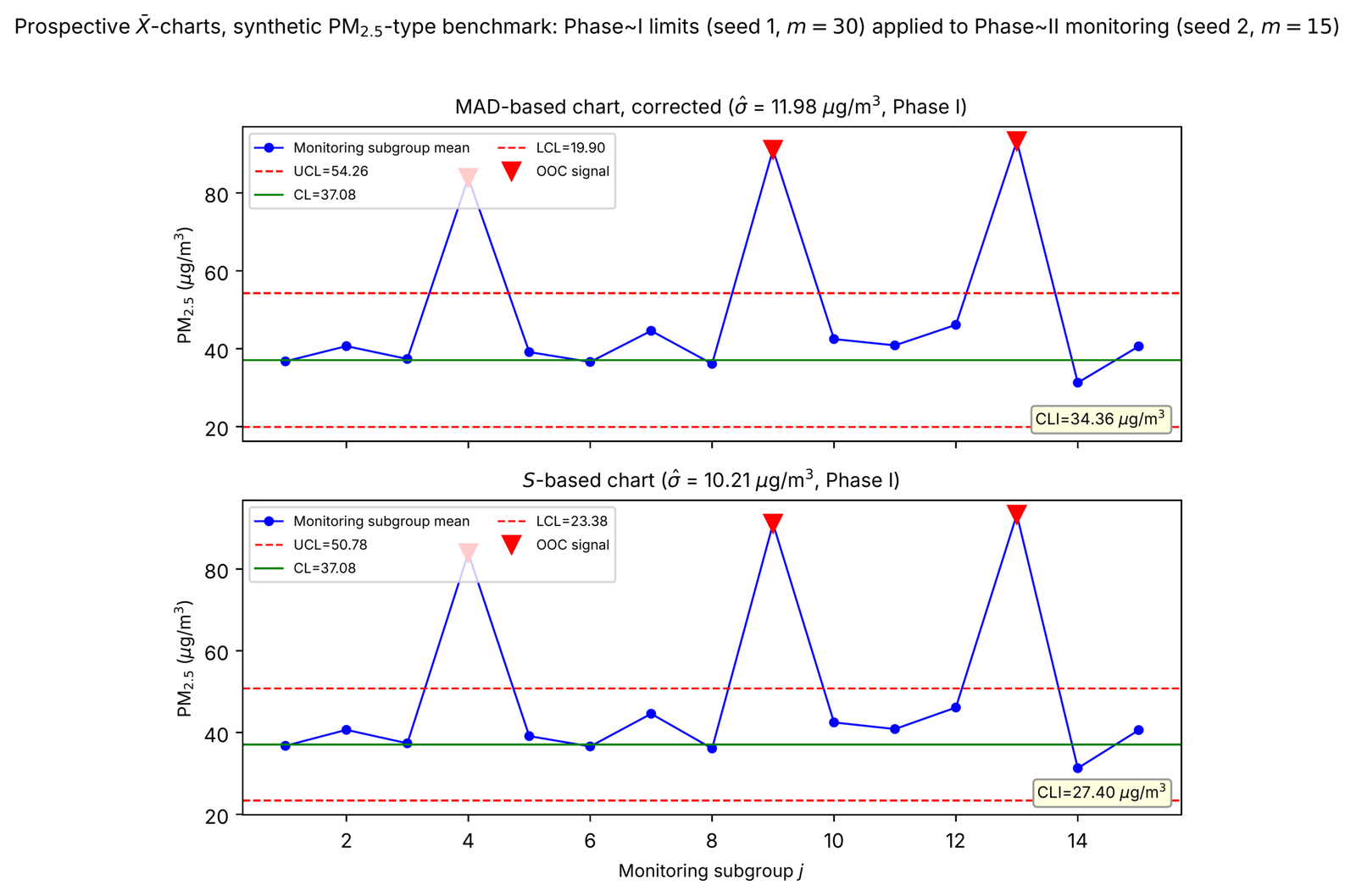
Design. Consistent with the operating context of §2.1, the benchmark uses two independent samples rather than one. A Phase I reference sample (default_rng(1), \(m=30\) subgroups of \(n=5\), generator printed in full in Appendix A) is drawn from the clean lognormal generator alone and used only to estimate the centre line and the three control limits (uncorrected MAD, corrected MAD, \(S\)); no disturbance is present in this sample. A separate Phase II monitoring sample (seed 2, \(m=15\) subgroups of \(n=5\), same clean generator) is then drawn independently, and three of its subgroups (4, 9, and 13) are multiplied by 2.4, emulating pollution episodes that scale both level and dispersion. The Phase I limits are applied to the Phase II subgroup means prospectively, exactly as defined by (1), rather than being re-estimated from the same data they are then checked against.
Generator. All values are rounded to two decimals exactly once, after any multiplicative episode has been applied (Appendix A). The reference data (Appendix Table 12) are moderately right-skewed (pooled skewness 0.99, excess kurtosis 2.38, Shapiro–Wilk \(W=0.951\), \(p<0.001\)); the monitoring data before prospective scoring (Appendix Table 13) are more strongly skewed once the episodes are included (skewness 1.56, kurtosis 3.14, \(W=0.871\), \(p<0.001\)). Lag-1 autocorrelation of the monitoring subgroup means is \(\hat\rho_1=-0.301\) (Ljung–Box \(Q=1.65\), \(p=0.20\)), providing no evidence of serial dependence at the stated significance level. Levene’s test across the monitoring subgroups does not reject homogeneity overall (\(F=0.66\), \(p=0.80\)), since only three of fifteen subgroups carry the injected episode.
Analysis with the Corrected Multiplier. All quantities below are computed from the exact observations of Tables 12–13 by the pooling rule of (9), applied in the two stages described above; text, tables, figures, and appendix are generated from a single stored result object. From the Phase I reference sample alone, \(\bar{\bar{X}}=37.08\), \(\hat\sigma_{\mathrm{MAD}}=d_5(\mathrm{MAD})\,\overline{\mathrm{MAD}}^{\dagger}=11.98\), and \(c^{*}(30,5)=1.0686\), hence \(A_6^{*}=1.6320\times1.0686=1.7439\):
The uncorrected MAD limits are 53.15 and 21.00 (CLI 32.15); the \(S\)-based chart (\(\hat\sigma_S=10.21\), \(A_3=1.4273\)) gives 50.78 and 23.38 (CLI 27.40), all estimated from the same Phase I reference sample. Applied prospectively to the Phase II monitoring subgroups, all three chart variants signal exactly the injected subgroups 4, 9, and 13, whose means 83.90, 91.11, and 93.32 \(\mu\)g/m\(^3\) lie far above every UCL (Table 6 and Figure 4). The episodes injected here are large relative to every chart’s control-limit interval, so all variants detect them; this benchmark illustrates the correct independent-sample mechanics of prospective monitoring under a strongly non-normal reference distribution, not a comparative detection claim between charts, which is the role of the replicated study of §3.4–3.6. Consistent with §2.2, no efficiency interpretation is attached to the fact that the \(S\)-based interval happens to be narrower here: under this skewed generator the two \(\hat\sigma\)’s estimate different functionals on one particular finite reference sample, and the width difference reflects the differing biases of normal-reference constants under lognormal-type data, not superior precision of either chart.
| Chart | \(\bar X\) | \(\hat\sigma\) | UCL | LCL | CLI | OOC subgroups |
|---|---|---|---|---|---|---|
| MAD-based, uncorrected (\(A_6\)) | 37.08 | 11.98 | 53.15 | 21.00 | 32.15 | 4, 9, 13 |
| MAD-based, corrected (\(A_6^{*}\)) | 37.08 | 11.98 | 54.26 | 19.90 | 34.36 | 4, 9, 13 |
| \(S\)-based | 37.08 | 10.21 | 50.78 | 23.38 | 27.40 | 4, 9, 13 |
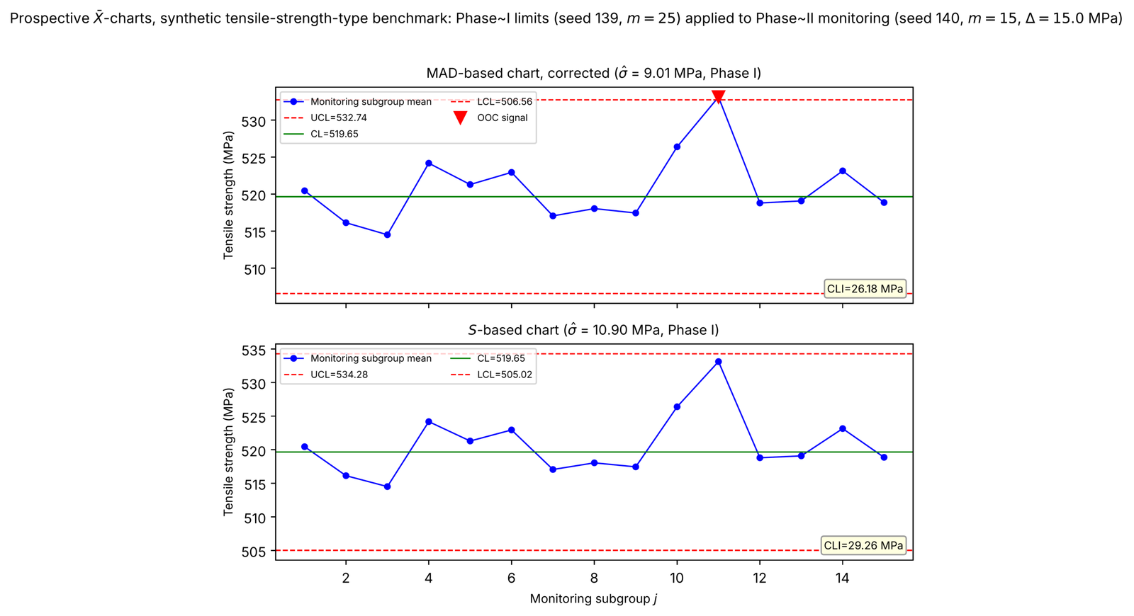
Design. As in Benchmark A, two independent samples are used. A Phase I reference sample (numpy.random.default_rng(139), \(m=25\) batches of \(n=5\), generator printed in Appendix A) is drawn from the clean Weibull-type generator, \(X_{ij}=520+11\,(W_{ij}-\mu_W)/s_W\) with \(W_{ij}\) standard Weibull of shape 1.5 and the exact constants of §3.2, and used only to estimate the centre line and the three control limits; it contains no injected shift. A separate Phase II monitoring sample (seed 140, \(m=15\) batches of \(n=5\), same clean generator) is then drawn independently, and a level shift of \(\Delta=+15.0\) MPa, approximately 1.4 population standard deviations of the generating process, is added to batches 4 and 11; \(\Delta\) is a stylised design choice fixed in advance of the monitoring draw, not a value fitted to it. The Phase I limits are applied to the Phase II batch means prospectively.
Generator. Values are rounded to two decimals exactly once, after any shift has been added. Reference data (Appendix Table 14) are right-skewed (pooled skewness 0.96, Shapiro–Wilk \(W=0.934\), \(p<0.001\)); the reported test does not detect serial dependence in the batch means (\(\hat\rho_1=0.013\), Ljung–Box \(p=0.95\)) and the variance test does not reject within-batch homogeneity (Levene \(F=0.50\), \(p=0.97\)). Monitoring data before scoring show similar properties (skewness 0.46, \(\hat\rho_1=0.14\), \(p=0.54\), Levene \(p=0.93\)).
Analysis. From the Phase I reference sample alone (Table 14), \(\bar{\bar{X}}=519.65\) MPa, \(\hat\sigma_{\mathrm{MAD}}=9.01\) MPa, and \(\hat\sigma_{S}=10.90\) MPa, a realisation of the general finding of §3.4 and 3.6 that, on any given finite sample under skewness, the two estimators can differ materially even with no contamination present. With \(c^{*}(25,5)=1.0825\) (\(A_6^{*}=1.7666\)):
while the \(S\)-based chart gives \(\mathrm{UCL}^{(S)}=534.28\), \(\mathrm{LCL}^{(S)}=505.02\) MPa. Applied prospectively to the Phase II monitoring sample (Table 15), the shifted batches have means \(\bar X_4=524.18\) and \(\bar X_{11}=533.12\) MPa: batch 11 exceeds both the corrected MAD-based UCL of 532.74 and the uncorrected UCL of 531.74 but falls short of the wider \(S\)-based UCL of 534.28, so the MAD-based charts signal it and the \(S\)-based chart does not; batch 4, whose own unshifted draw happened to fall below the reference centre line, is not flagged by any chart at this shift magnitude (Table 7, Figure 5). The correct description of the mechanism is not that the injected shift inflates \(\hat\sigma_S\): adding a constant to every observation in a batch leaves that batch’s own standard deviation and MAD unchanged, as it must. What differs is the width of each chart’s limits, fixed in Phase I before any shift is seen, and a shift that clears the narrower MAD-based interval but not the wider \(S\)-based one is accordingly caught by one chart and missed by the other. This single realisation illustrates, with one concrete numerical example, the general masking phenomenon quantified across replications in §3.4 and §3.6; it is not, by itself, evidence of a general detection advantage, and batch 4’s non-detection is reported here precisely because a single realisation need not illustrate the general pattern uniformly.
| Chart | \(\bar X\) | \(\hat\sigma\) | UCL | LCL | CLI | OOC subgroups |
|---|---|---|---|---|---|---|
| MAD-based, uncorrected (\(A_6\)) | 519.65 | 9.01 | 531.74 | 507.56 | 24.18 | 11 |
| MAD-based, corrected (\(A_6^{*}\)) | 519.65 | 9.01 | 532.74 | 506.56 | 26.18 | 11 |
| \(S\)-based | 519.65 | 10.90 | 534.28 | 505.02 | 29.26 | none |
Principal Findings. The calibrated comparison shows that under clean data, normal or skewed, the robust charts obtain their per-subgroup breakdown protection at a modest cost in detection efficiency and no detection advantage. An asymmetry survives clean data, however: under exponential-type skewness the high-breakdown charts are modestly to substantially slower than \(S\) at detecting negative shifts, shifts toward the model’s short tail, a genuine if secondary cost of robustness traced to the larger calibrated multiplier the robust estimators require under skewness. The contamination study shows where the robust charts genuinely dominate: with 10% location outliers in the reference sample, the \(S\)-based chart’s false-alarm calibration collapses by an order of magnitude and its median run length at a subsequent \(1\sigma_0\) shift lengthens roughly sixfold relative to the MAD chart, effectively stopping detection altogether. The practical implication is correspondingly sharpened: choose the MAD- or \(Q_n\)-based chart when contamination of the reference data cannot be excluded, not because the process is skewed.
Terminology. Parameter-estimation-adjusted continues to denote a one-time design-stage adjustment for finite-\(m\) estimation error, in the spirit of [14,22], as distinct from adaptive charts that update parameters in response to incoming data [18]. Change-point estimation for fixed or variable sampling charts is another distinct task [19].
Pre-Test Selection. Pre-testing normality to select between the \(S\)– and MAD-based charts introduces a two-stage selection effect that is difficult to control [9]. In the light of the calibrated results the guidance is refined: default to the MAD-based (or, for higher efficiency, \(Q_n\)-based) chart with the corrected multiplier whenever contamination of the Phase I data cannot be ruled out; if the reference data are known to be clean, the calibrated \(S\)-based chart is adequate under any of the shapes studied here, provided its multiplier is calibrated to the distribution actually in force.
Choice of Estimator. Among the estimators whose per-subgroup statistic attains the asymptotic breakdown point of 0.5 (MAD, \(S_n\), \(Q_n\); §2.6 qualifies what this does and does not imply for the pooled chart), \(Q_n\) offers the best efficiency–robustness balance (asymptotic ARE 82%, finite-\(n\) RE 45.5–63.3% at \(n=5\)–\(10\)) although its contaminated-sample detection is slightly slower than that of the MAD in the comparisons reported in Table 4; the closed-form correction (17) is derived for the MAD, but the calibration procedure of §3.4 applies to any of the six charts unchanged.
Limitations. The closed form (17) is a normal-theory, first-order-in-\(1/m\) result targeting the unconditional FAP; under strong skewness the location–scale covariance it neglects is nonzero and the numerically calibrated multiplier should be used, with \(\kappa_\tau^{2}\) (if the closed form is retained) estimated from pilot data, whose additional estimation uncertainty then propagates into the FAP. A conditional FAP guarantee requires a separate conditional calibration criterion; bootstrap adjustment provides one established approach [21]. Both benchmarks are balanced, serially independent, and synthetic; retrospective screening of the estimation sample itself, autocorrelated or unbalanced data, and multivariate, CUSUM, and EWMA extensions with high-breakdown scale estimators remain open.
This paper developed parameter-estimation-adjusted robust \(\bar X\)-charts based on the median absolute deviation for prospective monitoring with limits estimated from a finite Phase I reference sample under non-normal and contaminated processes. Starting from the correct unconditional FAP expression, in which the expectation runs over the joint law of the estimated centre line and scale, the corrected multiplier \(A_6^{*}=A_6\sqrt{1+1/m}\,\{1+9\kappa_\tau^{2}/(2mn)\}\), with the correctly normalised \(\kappa_\tau^{2}=n\,\mathrm{Var}(d_n\mathrm{MAD}_j)/\sigma_0^{2}\), was derived and proved to restore the nominal FAP up to \(O(m^{-2})\) under normality; Monte Carlo evidence with exact conditional signal probabilities and \(B=100{,}000\) replications confirms FAP within 12% of nominal at \(m=10\) and within 6% for \(m\ge15\). A unified limit formula with Monte-Carlo-verified finite-sample constants ensures every unbiasing constant appears exactly once. Comparisons across six estimators, four distributions, and both shift directions, made only after calibration to a common in-control FAP, show that robust charts incur a modest cost in detection efficiency under clean data, together with a secondary cost under exponential-type skewness of slower detection of negative shifts, while a dedicated \(\varepsilon\)-contamination study shows the classical \(S\)-based chart’s calibration and detection collapsing under 5–10% scattered reference-sample contamination that the robust charts absorb far better, a resistance that – as §2.6 qualifies – reflects their performance under this specific contamination arrangement rather than a pooled breakdown point of 0.5. Two fully documented synthetic benchmarks, analysed with the corrected limits, an independent Phase I/Phase II split, and recomputable line by line from the printed observations, illustrate the mechanics of prospective monitoring under a strongly non-normal reference distribution and, in a single numerical realisation, the masking of an injected shift by the \(S\)-based chart under Weibull-type data.
Practical guidance. Use the MAD-based chart with \(A_6^{*}\) from (17), or the \(Q_n\)-based chart for higher efficiency, whenever the Phase I reference data may be contaminated; calibrate the multiplier per distribution when the in-control shape is known and strongly non-normal. Future research should formulate the fully retrospective (leave-one-out) Phase I screening problem for high-breakdown estimators, quantify the covariance correction under skewness, and extend the framework to multivariate, CUSUM, and EWMA schemes.
Author Contributions: Both authors contributed equally to this work and approved the final manuscript.
Conflicts of Interest: The authors declare no conflict of interest.
Data Availability: The synthetic benchmark observations and their generating code are included in Appendix A. No externally collected observational datasets were used for these benchmarks.
Funding Information: No funding was received for this research.
Data. The reference and monitoring subgroup means for Benchmark A appear in Tables 8 and 9, respectively. The corresponding batch means for Benchmark B appear in Tables 10 and 11. Raw observations for the two phases of Benchmark A are listed in Tables 12 and 13; those for Benchmark B are listed in Tables 14 and 15. Together, these tables list all subgroup means and every raw observation of both benchmarks’ Phase I reference and Phase II monitoring samples, exactly as analysed (rounded to two decimals after any injected episode, shift, or other disturbance has been applied, so the printed values reproduce the reported results to the last digit). Code. A master script (master.py) regenerates, in order, the constants of Table 1 (seed 20260501), the FAP study of Table 2 (seed \(31000+m\) for each reference-sample size \(m\)), the calibrated study of Table 3 (seed \(41000+100i_{\mathrm{dist}}+10i_n+i_{\mathrm{est}}\), with \(i_{\mathrm{dist}}\in\{0,1,2,3\}\) indexing the four distributions in the order Normal, Exponential, \(\chi^2_3\), Weibull\((1.5)\), \(i_n\in\{0,1\}\) indexing \(n\in\{5,10\}\), and \(i_{\mathrm{est}}\in\{0,\dots,5\}\) indexing the six estimators in the order \(S\), MAD, \(S_n\), \(Q_n\), Trim, Win), the contamination study of Table 4 (seed \(51000+i\), \(i\) incrementing once per contamination-model/estimator cell in the fixed loop order \(H\in\{N(4,1),N(0,9)\}\), \(\varepsilon\in\{0.05,0.10\}\), estimator in the same six-estimator order), both benchmarks (Phase I reference seeds 1 and 139, Phase II monitoring seeds 2 and 140), and Figures 1–5 (seeds 61000–63000 series, offsets detailed in the script itself); every table and figure is written from the same stored JSON result objects, with no manual intervention. Every calibration bisection (the multiplier \(\hat\lambda\) of §3.4 and the width-scaling search of §3.2) runs a fixed 60 halving iterations, giving a multiplier precision better than \(10^{-15}\), i.e. exact to floating-point precision; no calibration tolerance is otherwise imposed. The median run length \(\eta\) of §2.6 is located by bisection on the exact closed form \(S(k)=\mathrm{mean}\{\exp(k\log(1-p_{\hat\theta}))\}\) to the same precision. Software: Python 3, NumPy 2.4.4, SciPy 1.17.1, Matplotlib 3.10.8. The two benchmark generators are, in full:
import numpy as np
# Benchmark A (PM2.5-type): Phase I reference, m=30, n=5
rng = np.random.default_rng(1)
Xref = np.round(np.exp(rng.normal(3.60, 0.32, size=(30, 5))), 2)

# Benchmark A: Phase II monitoring, m=15, n=5, independent sample
rng = np.random.default_rng(2)
Xmon = np.exp(rng.normal(3.60, 0.32, size=(15, 5)))
for j in (3, 8, 12):   # monitoring subgroups 4, 9, 13
    Xmon[j] = Xmon[j] * 2.4
Xmon = np.round(Xmon, 2)   # rounded once, after the episode

# Benchmark B (tensile-strength-type): Phase I reference, m=25, n=5
mu_w = 0.902745; s_w = 0.612936          # rounded Weibull(1.5) constants
rng = np.random.default_rng(139)
Wref = (rng.weibull(1.5, size=(25, 5)) - mu_w) / s_w
Yref = np.round(520.0 + 11.0 * Wref, 2)

# Benchmark B: Phase II monitoring, m=15, n=5, independent sample
rng = np.random.default_rng(140)
Wmon = (rng.weibull(1.5, size=(15, 5)) - mu_w) / s_w
Ymon = 520.0 + 11.0 * Wmon
for j in (3, 10):     # monitoring batches 4, 11
    Ymon[j] = Ymon[j] + 15.0
Ymon = np.round(Ymon, 2) # rounded once, after the shift| \(j\) | \(\bar X_j\) | \(j\) | \(\bar X_j\) | \(j\) | \(\bar X_j\) | \(j\) | \(\bar X_j\) |
|---|---|---|---|---|---|---|---|
| 1 | 40.44 | 9 | 30.48 | 17 | 36.22 | 25 | 45.20 |
| 2 | 39.69 | 10 | 39.76 | 18 | 39.33 | 26 | 30.88 |
| 3 | 35.11 | 11 | 38.93 | 19 | 41.73 | 27 | 36.57 |
| 4 | 35.39 | 12 | 33.80 | 20 | 30.74 | 28 | 30.04 |
| 5 | 38.29 | 13 | 33.72 | 21 | 42.50 | 29 | 39.84 |
| 6 | 33.00 | 14 | 35.79 | 22 | 38.20 | 30 | 34.65 |
| 7 | 49.10 | 15 | 40.38 | 23 | 37.44 | ||
| 8 | 34.88 | 16 | 34.27 | 24 | 36.00 |
| \(j\) | \(\bar X_j\) | \(j\) | \(\bar X_j\) | \(j\) | \(\bar X_j\) |
|---|---|---|---|---|---|
| 1 | 36.75 | 6 | 36.60 | 11 | 40.86 |
| 2 | 40.67 | 7 | 44.60 | 12 | 46.13 |
| 3 | 37.37 | 8 | 36.11 | 13 | 93.32 |
| 4 | 83.90 | 9 | 91.11 | 14 | 31.29 |
| 5 | 39.14 | 10 | 42.48 | 15 | 40.61 |
| \(j\) | \(\bar X_j\) | \(j\) | \(\bar X_j\) | \(j\) | \(\bar X_j\) | \(j\) | \(\bar X_j\) |
|---|---|---|---|---|---|---|---|
| 1 | 524.38 | 8 | 526.00 | 15 | 520.46 | 22 | 528.20 |
| 2 | 515.59 | 9 | 517.86 | 16 | 515.97 | 23 | 512.59 |
| 3 | 511.31 | 10 | 513.95 | 17 | 524.79 | 24 | 519.46 |
| 4 | 521.31 | 11 | 514.34 | 18 | 518.25 | 25 | 522.02 |
| 5 | 519.82 | 12 | 521.43 | 19 | 513.03 | ||
| 6 | 524.82 | 13 | 523.57 | 20 | 516.39 | ||
| 7 | 519.93 | 14 | 522.96 | 21 | 522.84 |
| \(j\) | \(\bar X_j\) | \(j\) | \(\bar X_j\) | \(j\) | \(\bar X_j\) | \(j\) | \(\bar X_j\) |
|---|---|---|---|---|---|---|---|
| 1 | 524.38 | 8 | 526.00 | 15 | 520.46 | 22 | 528.20 |
| 2 | 515.59 | 9 | 517.86 | 16 | 515.97 | 23 | 512.59 |
| 3 | 511.31 | 10 | 513.95 | 17 | 524.79 | 24 | 519.46 |
| 4 | 521.31 | 11 | 514.34 | 18 | 518.25 | 25 | 522.02 |
| 5 | 519.82 | 12 | 521.43 | 19 | 513.03 | ||
| 6 | 524.82 | 13 | 523.57 | 20 | 516.39 | ||
| 7 | 519.93 | 14 | 522.96 | 21 | 522.84 |
| \(j\) | \(X_{1j}\) | \(X_{2j}\) | \(X_{3j}\) | \(X_{4j}\) | \(X_{5j}\) |
|---|---|---|---|---|---|
| 1 | 40.88 | 47.60 | 40.68 | 24.12 | 48.90 |
| 2 | 42.22 | 30.82 | 44.08 | 41.13 | 40.21 |
| 3 | 36.93 | 43.60 | 28.91 | 34.74 | 31.37 |
| 4 | 44.33 | 37.07 | 33.33 | 28.50 | 33.71 |
| 5 | 36.69 | 33.51 | 55.37 | 50.51 | 15.37 |
| 6 | 20.00 | 34.61 | 31.97 | 39.19 | 39.23 |
| 7 | 72.08 | 25.64 | 32.43 | 70.36 | 45.01 |
| 8 | 45.25 | 31.05 | 21.60 | 38.61 | 37.90 |
| 9 | 24.71 | 29.41 | 35.76 | 27.05 | 35.47 |
| 10 | 37.73 | 37.02 | 31.12 | 44.26 | 48.68 |
| 11 | 40.56 | 28.17 | 46.25 | 31.17 | 48.49 |
| 12 | 25.97 | 49.04 | 36.36 | 24.54 | 33.10 |
| 13 | 37.24 | 39.94 | 26.73 | 25.68 | 39.01 |
| 14 | 31.52 | 39.46 | 46.67 | 21.59 | 39.70 |
| 15 | 54.16 | 33.27 | 28.23 | 46.56 | 39.69 |
| 16 | 48.75 | 32.77 | 22.78 | 35.33 | 31.73 |
| 17 | 46.90 | 38.94 | 21.72 | 24.97 | 48.56 |
| 18 | 45.49 | 29.82 | 36.59 | 42.21 | 42.52 |
| 19 | 48.44 | 39.73 | 35.50 | 33.69 | 51.31 |
| 20 | 17.81 | 35.01 | 36.99 | 23.19 | 40.71 |
| 21 | 29.71 | 48.23 | 35.16 | 45.34 | 54.06 |
| 22 | 41.37 | 27.65 | 22.54 | 64.14 | 35.32 |
| 23 | 29.36 | 38.33 | 34.42 | 48.07 | 37.00 |
| 24 | 36.76 | 29.12 | 42.53 | 26.29 | 45.29 |
| 25 | 59.60 | 22.47 | 16.62 | 44.59 | 82.71 |
| 26 | 26.57 | 24.53 | 44.19 | 27.97 | 31.13 |
| 27 | 32.74 | 43.39 | 32.15 | 40.00 | 34.59 |
| 28 | 27.93 | 33.04 | 27.00 | 36.67 | 25.54 |
| 29 | 25.80 | 58.34 | 35.98 | 35.97 | 43.11 |
| 30 | 31.99 | 34.02 | 41.93 | 40.06 | 25.26 |
| \(j\) | \(X_{1j}\) | \(X_{2j}\) | \(X_{3j}\) | \(X_{4j}\) | \(X_{5j}\) |
|---|---|---|---|---|---|
| 1 | 38.88 | 30.96 | 32.07 | 16.76 | 65.10 |
| 2 | 52.78 | 32.98 | 46.88 | 40.04 | 30.65 |
| 3 | 50.04 | 33.14 | 32.94 | 28.40 | 42.33 |
| 4 | 85.09 | 104.58 | 72.32 | 91.47 | 66.02 |
| 5 | 47.91 | 38.87 | 40.68 | 41.74 | 26.48 |
| 6 | 47.02 | 70.68 | 21.67 | 21.04 | 22.61 |
| 7 | 47.91 | 38.14 | 51.68 | 46.12 | 39.15 |
| 8 | 40.08 | 34.66 | 48.32 | 25.50 | 31.98 |
| 9 | 94.94 | 156.32 | 68.77 | 62.19 | 73.35 |
| 10 | 49.91 | 33.95 | 55.91 | 20.10 | 52.52 |
| 11 | 50.97 | 23.24 | 38.44 | 54.00 | 37.64 |
| 12 | 50.40 | 78.25 | 39.95 | 33.46 | 28.60 |
| 13 | 108.08 | 82.48 | 82.95 | 84.93 | 108.14 |
| 14 | 26.02 | 22.43 | 16.80 | 53.71 | 37.47 |
| 15 | 59.34 | 36.49 | 28.86 | 42.65 | 35.71 |
| \(j\) | \(X_{1j}\) | \(X_{2j}\) | \(X_{3j}\) | \(X_{4j}\) | \(X_{5j}\) |
|---|---|---|---|---|---|
| 1 | 513.26 | 545.58 | 512.80 | 512.40 | 537.88 |
| 2 | 505.57 | 515.29 | 528.32 | 518.14 | 510.61 |
| 3 | 509.12 | 508.77 | 509.51 | 522.91 | 506.23 |
| 4 | 512.46 | 526.50 | 529.76 | 507.90 | 529.91 |
| 5 | 505.70 | 527.36 | 511.10 | 534.22 | 520.72 |
| 6 | 535.28 | 540.29 | 505.57 | 511.42 | 531.56 |
| 7 | 524.32 | 536.41 | 505.25 | 526.94 | 506.72 |
| 8 | 548.13 | 511.55 | 515.41 | 518.02 | 536.88 |
| 9 | 508.80 | 533.61 | 515.08 | 516.84 | 514.98 |
| 10 | 528.16 | 508.29 | 516.02 | 507.75 | 509.51 |
| 11 | 508.19 | 507.17 | 524.77 | 509.99 | 521.58 |
| 12 | 526.63 | 515.81 | 529.99 | 516.61 | 518.12 |
| 13 | 516.86 | 509.12 | 516.28 | 562.55 | 513.03 |
| 14 | 513.19 | 518.81 | 519.97 | 533.44 | 529.39 |
| 15 | 545.31 | 525.72 | 514.16 | 504.62 | 512.48 |
| 16 | 513.45 | 518.93 | 518.71 | 520.50 | 508.28 |
| 17 | 521.20 | 527.87 | 526.39 | 532.75 | 515.74 |
| 18 | 531.58 | 508.46 | 522.04 | 507.99 | 521.17 |
| 19 | 509.71 | 526.87 | 508.49 | 514.72 | 505.34 |
| 20 | 513.44 | 516.11 | 512.17 | 511.83 | 528.42 |
| 21 | 538.72 | 510.92 | 516.96 | 519.80 | 527.78 |
| 22 | 535.65 | 521.62 | 529.42 | 530.04 | 524.28 |
| 23 | 504.28 | 512.00 | 518.10 | 508.36 | 520.23 |
| 24 | 519.51 | 507.87 | 525.97 | 529.68 | 514.28 |
| 25 | 519.06 | 517.96 | 511.61 | 540.99 | 520.48 |
| \(j\) | \(X_{1j}\) | \(X_{2j}\) | \(X_{3j}\) | \(X_{4j}\) | \(X_{5j}\) |
|---|---|---|---|---|---|
| 1 | 516.95 | 518.35 | 516.29 | 508.41 | 542.25 |
| 2 | 516.00 | 512.24 | 522.72 | 508.92 | 520.78 |
| 3 | 507.96 | 524.20 | 505.24 | 516.94 | 518.20 |
| 4 | 526.75 | 524.14 | 522.76 | 527.75 | 519.49 |
| 5 | 524.11 | 534.87 | 521.11 | 510.88 | 515.50 |
| 6 | 519.86 | 521.17 | 534.00 | 526.87 | 512.80 |
| 7 | 512.30 | 520.54 | 525.18 | 512.01 | 515.24 |
| 8 | 508.29 | 511.41 | 541.52 | 513.81 | 515.19 |
| 9 | 505.79 | 536.19 | 517.21 | 506.73 | 521.31 |
| 10 | 518.61 | 521.42 | 529.42 | 539.36 | 523.14 |
| 11 | 534.16 | 521.49 | 540.03 | 530.95 | 538.96 |
| 12 | 517.72 | 528.14 | 536.12 | 504.10 | 507.91 |
| 13 | 519.64 | 506.67 | 526.93 | 530.66 | 511.50 |
| 14 | 541.40 | 511.30 | 530.57 | 515.53 | 516.91 |
| 15 | 530.87 | 509.49 | 513.54 | 522.52 | 517.90 |