
The delay differential equations (DDEs) are a sort of ordinary differential equations in which the derivative of an unknown function at a specific time is expressed in terms of the of the function’s prior values. Which are widely used in mathematical modeling, including population dynamics, chemical kinetics, physiological and pharmaceutical kinetics, and infectious diseases kinetics. A simplest form of time-delay differential equations for \(y(t)\) is
\[\label{eq1} y'\left(t\right)=f\left(t,y\left(t\right),y\left(qt\right)\right), \tag{1}\] where \(q\) is a constant delay and \(f\) is well-defined function.
Fractional calculus is employed in many disciplines of applied mathematics because to may be used to simulate diverse physical processes in engineering and science. This has many uses in serval sectors of sciences. Example include, the dynamics of viscoelastic materials [1], electromagnetism [2], fluid mechanics [3], propagation of spherical flames [4], and viscoelastic materials [5].
In the literature, the authors discussed the solutions for nonlinear fractional delay differential equations with different analytical and numerical methods [6– 17]. Recently the authors in [18] have successfully implemented the Chebyshev pseudo-spectral method to solve fractional pantograph delay differential equations (FPDDEs). The fractional Taylor’s series (FTS) and the reproducing kernel method (RKs) are successfully used to solve a class of PDDEs by Du in [19]. Saeed et al. [20] established a technique by combining both the method of steps and the Hermite wavelet method for solving the fractional delay differential equations. Yang et al. [21] suggested the Jacobi collocation method (JCM) to solve FPDDEs. Dehestani et al. [22] followed the fractional-order hybrid Bessel functions (FHBFs) to obtain a numerical solution for fractional generalized pantograph-delay differential equations. Hashemia et al. [23] engaged the generalized squared remainder minimization method (GSRM) to find the solution for the FPDDEs. Yuttanan et al. [24] proposed a numerical technique called the fractional-order generalized Taylor wavelet method for nonlinear fractional delay and nonlinear fractional pantograph differential equations. More recently, Jassim & Abdulshareef [25] proposed a new iterative method for solving linear and nonlinear problems of ordinary fractional differential equations, namely the Hussein–Jassim method (HJM). The concept of this method is based on a power series of fractional order. In this study, we solve a class of time-delay differential equations with the Caputo fractional-order by using the Hussein–Jassim method.
The remainder of this paper is structured as follows: A few basic definitions related to fractional calculus are given in Section 2. Section 3 presents the procedures to use the HJM for solving differential equation. Some examples are discussed in Section 4. Furthermore, a conclusion is provided in the last section.
In this section, we mention several concepts and definitions which are needed later in this paper.
Definition 1. [25, 26] The Riemann–Liouville fractional integral of order \(v>0,\) is defined as: \[\label{eq2} J^vy\left(t\right) {=}\frac{v}{ {\Gamma}\left(v+1\right)}\int^t_0{\frac{y\left(\tau \right)}{{\left(t {-}\tau \right)}^{1-v}}}d\tau , \tag{2}\] where \(\Gamma\) is the well-known Gamma function.
Useful properties of the Riemann–Liouville fractional integral are as follows:
\(J^0y\left(t\right)=y\left(t\right),\)
\(J^v\left[y\left(t\right)+x(t)\right]=J^v\left[y\left(t\right)\right]+J^v\left[x(t)\right],\)
\(J^vJ^uy\left(t\right)=J^{v+u}y\left(t\right)=J^uJ^vy\left(t\right),\)
\(J^vt^{\alpha }=\frac{ {\Gamma}\left(\alpha +1\right)}{ {\Gamma}\left(v+\alpha +1\right)}t^{v+\alpha }.\)
Definition 2. [25, 26] The formula for the Caputo fractional derivative of \(y\left(t\right),\) is defined as:
\[\label{eq3} {}^c_a{{\mathcal{D}}^v_t}y\left(t\right)=\frac{1}{ {\Gamma}\left(m-v\right)}\int^t_0{{\left(t-\tau \right)}^{m-v\ -\ 1}y^{\left(m\right)}\left(\tau \right)}d\tau ,\quad \quad m-1< {\ }v\le m. \tag{3}\]
The properties of the Caputo fractional operator are as follows:
\({}^c_a{{\mathcal{D}}^v_t}K=0,\) where \(K\) is constant.
\({}^c_a{{\mathcal{D}}^v_t}\left[y\left(t\right)+x(t)\right]={}^c_a{{\mathcal{D}}^v_t}\left[y\left(t\right)\right]+{}^c_a{{\mathcal{D}}^v_t}\left[x(t)\right],\)
\({}^c_a{{\mathcal{D}}^v_t}J^vy\left(t\right)=y\left(t\right),\)
\({}^c_a{{\mathcal{D}}^v_t}t^{\alpha }=\frac{ {\Gamma}\left(\alpha +1\right)}{ {\Gamma}\left(\alpha -v+1\right)}t^{v+\alpha }.\)
Definition 3. [25, 26] The Special function called Mittag–Leffler function denoted as \(E_v\left(t\right),\) is defined as: \[\label{eq4} E_v\left(t\right)=\sum^{\infty }_{n=0}{\frac{t^n}{ {\Gamma }\left(vn+1\right)}}. \tag{4}\]
Specifically, for different values of \(v\) we have the following functions:
\(E_0\left(t\right)=\frac{1}{1-t},\)
\(E_1\left(t\right)=e^t,\)
\(E_2\left(t^2\right)={ {cosh} t\ }.\)
Consider the following fractional differential equation
\[\label{eq5} {}^c{{\mathcal{D}}^v_t}y\left(t\right)=f\left(t\right)+\mathcal{M}\left[y\left(t\right)\right],\quad \quad 0< {\ }v\le 1, \tag{5}\] with initial condition \[\label{eq6} y\left(0\right)=\omega , \tag{6}\] where \({}^c{{\mathcal{D}}^v_t} {(.)}\) is the Caputo fractional derivative, \(\mathcal{M}\) is a nonlinear operator, \(y\) is an analytical function, and \(f\left(t\right)\) is a known function.
Applying the integral operator \(J^v\) to (5) gives an algebraic equation as \[y\label{eq7} \left(t\right)=\omega +J^vf\left(t\right)+J^v\left[\mathcal{M}\left[y\left(t\right)\right]\right]. \tag{7}\]
We consider the RHS of (7) as an infinite series representation of the Mittag-Leffler function, we have \[\label{eq8} \omega {+}J^vf\left(t\right)+J^v\left[\mathcal{M}(\left(y\left(t\right)\right)\right]=a_0+\frac{a_1}{ {\Gamma }\left(v+1\right)}t^v+\frac{a_2}{ {\Gamma }\left(2v+1\right)}t^{2v}+\dots =\sum^{\infty }_{j=0}{\frac{a_jt^{jv}}{ {\Gamma }\left(jv+1\right)}}, \tag{8}\] where \(a_{ {j}} {,\ j} {\ge } {0,}\) are constants.
The constants coefficients \(a_{ {j}},\) can be attained by taking the differential operator \({}^c{{\mathcal{D}}^{jv}_t},\ j\ge 0,\) into (8) at \(t=0,\) which gives
\[\label{eq9} \begin{cases} a_0=\omega , \\ a_1=f\left(t\right){\left.+\mathcal{M}\left[y\left(t\right)\right]\right|}_{t=0}, \\ a_2={\left.{}^c{{\mathcal{D}}^v_t}\left(f\left(t\right)+\mathcal{M}\left[y\left(t\right)\right]\right)\right|}_{t=0}, \\ a_3={\left.{}^c{{\mathcal{D}}^{2v}_t}\left(f\left(t\right)+\mathcal{M}\left[y\left(t\right)\right]\right)\right|}_{t=0}, \\ \vdots \end{cases} \tag{9}\]
Substituting (9) into (8) we have \[\label{e10} y\left(t\right)=\sum^{\infty }_{j=0}{\frac{{\left.{}^c{{\mathcal{D}}^{(j-1)v}_t}\left(f\left(t\right)+\mathcal{M}\left[y\left(t\right)\right]\right)\right|}_{t=0}}{ {\Gamma }\left(jv+1\right)}t^{jv}}. \tag{10}\]
Assume that the solution of (10), given by \[\label{eq11} y\left(t\right)=\sum^{\infty }_{j=0}{y_j\left(t\right)}. \tag{11}\]
Substituting (11) into (10) we obtain \[\label{eq12} \sum^{\infty }_{j=0}{y_j\left(t\right)}=\sum^{\infty }_{j=0}{\frac{{\left.\left[{}^c{{\mathcal{D}}^{\left(j-1\right)v}_t}\left(f(t)+\mathcal{M}\left(\sum^{\infty }_{j=0}{y_j\left(t\right)}\right)\right)\right]\right|}_{t=0}}{ {\Gamma }\left(jv+1\right)}t^{jv}}. \tag{12}\]
Replace \(j\) by \(j+1\) in the left side of (12), we get \[\label{eq13} y_0\left(t\right)+\sum^{\infty }_{j=0}{y_{j+1}\left(t\right)}=\omega +\sum^{\infty }_{j=0}{\frac{{\left.{}^c{{\mathcal{D}}^{\left(j-1\right)v}_t}\left(f(t)+\mathcal{M}\left(\sum^{\infty }_{j=0}{y_j\left(t\right)}\right)\right)\right|}_{t=0}}{ {\Gamma }\left(jv+1\right)}t^{jv}}. \tag{13}\]
Thus, the following relation is obtained by compare the two sides of (13) \[\label{eq14} \begin{cases} y_0(t)=\omega , \\ y_1(t)=\frac{{\left.\left(f\left(t\right)+\mathcal{M}(y_0\left(t\right))\right)\right|}_{t=0}}{ {\Gamma }\left(v+1\right)}t^v, \\ y_2(t)=\frac{{\left.{}^c{{\mathcal{D}}^v_t}\left(f\left(t\right)+\mathcal{M}\left(y_0\left(t\right)+y_1\left(t\right)\right)\right)\right|}_{t=0}}{ {\Gamma }\left(2v+1\right)}t^{2v}, \\ y_3(t)=\frac{{\left.{}^c{{\mathcal{D}}^{2v}_t}\left(f\left(t\right)+\mathcal{M}\left(y_0\left(t\right)+y_1\left(t\right)+y_2\left(t\right)\right)\right)\right|}_{t=0}}{ {\Gamma }\left(3v+1\right)}t^{3v}, \\ \vdots \\ y_{j+1}(t)=\frac{{\left.{}^c{{\mathcal{D}}^{jv}_t}\left(f(t)+\mathcal{M}\left(y_0\left(t\right)+y_1\left(t\right)+y_2\left(t\right)+\dots +y_j\left(t\right)\right)\right)\right|}_{t=0}}{ {\Gamma }\left((j+1)v+1\right)}t^{(j+1)v}. \end{cases} \tag{14}\]
Consequently, the approximate solution is given by: \[\label{eq15} y_{HJM}\left(t\right)=y_0\left(t\right)+y_1\left(t\right)+y_2\left(t\right)+\dots =\sum^{\infty }_{j=0}{y_j\left(t\right)}. \tag{15}\]
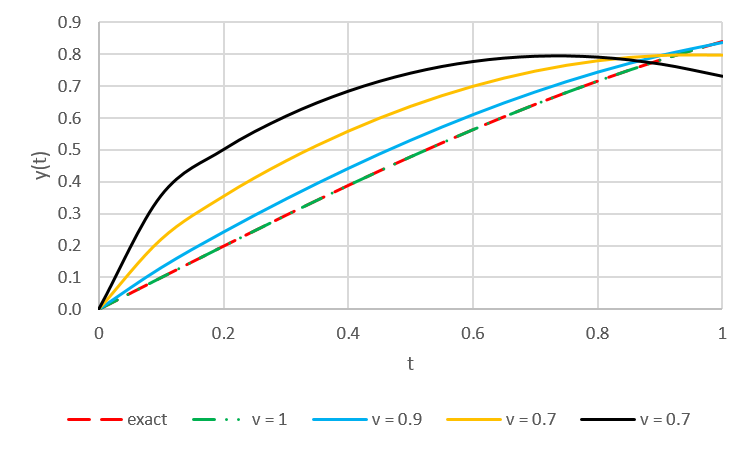
Example 1. Frist, we consider the nonlinear fractional delay differential equations [27] \[\label{eq16} {}^c{{\mathcal{D}}^v_t}y\left(t\right)=1-2y^2\left(\frac{t}{2}\right),\ \ y\left(0\right)=0. \tag{16}\]
For \(v=1\) the exact solution is given by \(y\left(t\right)={ {sin} t\ }.\)
According to (14), we get \[\label{17} \begin{cases} y_0\left(t\right)=0,\\ y_1\left(t\right)=\frac{t^v}{ {\Gamma }\left(v+1\right)}, \\ y_2\left(t\right)=0,\\ y_3\left(t\right)=-\frac{ {2} {\Gamma }\left(2v+1\right)t^{3v}}{2^{2v}{ {\Gamma }}^2\left(v+1\right) {\Gamma }\left(3v+1\right)},\\ y_4\left(t\right)=0,\\ y_5\left(t\right)=\frac{8 {\Gamma }\left(2v+1\right) {\Gamma }\left(4v+1\right)}{2^{6v}{ {\Gamma }}^3\left(v+1\right) {\Gamma }\left(3v+1\right) {\Gamma }\left(5v+1\right)}t^{5v}.\end{cases} \tag{17}\]
Therefore, According to these approximations, the 5\({}^{th}\) approximation solution of (16) is given by \[\label{eq18} y_{HJM}\left(t\right)=\frac{t^v}{ {\Gamma }\left(v+1\right)}-\frac{ {2} {\Gamma }\left(2v+1\right)t^{3v}}{2^{2v}{ {\Gamma }}^2\left(v+1\right) {\Gamma }\left(3v+1\right)}+\frac{8 {\Gamma }\left(2v+1\right) {\Gamma }\left(4v+1\right)}{2^{6v}{ {\Gamma }}^3\left(v+1\right) {\Gamma }\left(3v+1\right) {\Gamma }\left(5v+1\right)}t^{5v}. \tag{18}\]
Obviously, at \(v=1\) the solution is tends to an exact solution\(\ y\left(t\right)={ {sin} t\ }\).
The absolute error between exact solution and 5\({}^{th}\) approximation solution obtained by HJM when \(v=1\) are shown in Table 1. The corresponding numerical values of approximation solutions for different values of\(\ v\) are present in Table 2. The graphs of exact and approximation solutions for some values of\(\ v\) are shown in Figure 1.
| \(t\) | exact solution | approximation solution | absolute error |
| 0 | 0.0000000000 | 0.0000000000 | 0.0000000000 |
| 0.1 | 0.0998334166 | 0.0998334167 | 0.0000000000 |
| 0.2 | 0.1986693308 | 0.1986693333 | 0.0000000025 |
| 0.3 | 0.2955202067 | 0.2955202500 | 0.0000000433 |
| 0.4 | 0.3894183423 | 0.3894186667 | 0.0000003244 |
| 0.5 | 0.4794255386 | 0.4794270833 | 0.0000015447 |
| 0.6 | 0.5646424734 | 0.5646480000 | 0.0000055266 |
| 0.7 | 0.6442176872 | 0.6442339167 | 0.0000162294 |
| 0.8 | 0.7173560909 | 0.7173973333 | 0.0000412424 |
| 0.9 | 0.7833269096 | 0.7834207500 | 0.0000938404 |
| 1 | 0.8414709848 | 0.8416666667 | 0.0001956819 |
| \(t\) | \(v=1\) | \(v=0.9\) | \(v=0.7\) | \(v=0.5\) |
| 0 | 0.0000000000 | 0.0000000000 | 0.0000000000 | 0.0000000000 |
| 0.1 | 0.0998334167 | 0.1306801502 | 0.2192461496 | 0.3563467372 |
| 0.2 | 0.1986693333 | 0.2425293257 | 0.3539955899 | 0.5008213286 |
| 0.3 | 0.2955202500 | 0.3460040116 | 0.4646485205 | 0.6053060105 |
| 0.4 | 0.3894186667 | 0.4420524933 | 0.5579779714 | 0.6838326272 |
| 0.5 | 0.4794270833 | 0.5304811159 | 0.6358657931 | 0.7405628248 |
| 0.6 | 0.5646480000 | 0.6107378048 | 0.6987050867 | 0.7769184826 |
| 0.7 | 0.6442339167 | 0.6821544353 | 0.7463647620 | 0.7934715508 |
| 0.8 | 0.7173973333 | 0.7440548921 | 0.7785881405 | 0.7906972457 |
| 0.9 | 0.7834207500 | 0.7958160730 | 0.7952021853 | 0.7693641881 |
| 1 | 0.8416666667 | 0.8369088357 | 0.7962488772 | 0.7307805928 |
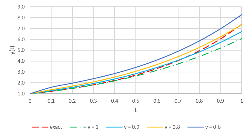
Example 2. Finally, we consider the fractional nonlinear neutral delay differential equation \[\label{eq19} {}^c{{\mathcal{D}}^v_t}y\left(t\right)=y\left(t\right)+y^2\left(\frac{t}{2}\right),\ \ y\left(0\right)=1, \tag{19}\] where \(t\ge 0,\) and \(0<v\le 1.\)
For \(v=1\) the exact solution is given by \(y\left(t\right)=e^{2t}.\)
According to (14), we get \[\label{20} \begin{cases} y_0\left(t\right)=1,\\ y_1\left(t\right)=\frac{2}{ {\Gamma }\left(v+1\right)}t^v,\\ y_2\left(t\right)=\frac{(2+\frac{4}{2^v})}{ {\Gamma }\left(2v+1\right)}t^{2v},\\ y_3\left(t\right)=\left[\left(2+\frac{4}{2^v}\right)\left(1+\frac{2}{2^{2v}}\right)+\frac{ {4} {\Gamma }\left(2v+1\right)}{2^{2v}{ {\Gamma }}^2\left(v+1\right)}\right]\frac{t^{3v}}{ {\Gamma }\left(3v+1\right)}. \end{cases} \tag{20}\]
Therefore, According to these approximations, the 3\({}^{rd}\) approximation solution of (16) is given by \[\label{eq21} y_{HJM}\left(t\right)=1+\frac{2}{ {\Gamma }\left(v+1\right)}t^v+\frac{(2+\frac{4}{2^v})}{ {\Gamma }\left(2v+1\right)}t^{2v}+\left[\left(2+\frac{4}{2^v}\right)\left(1+\frac{2}{2^{2v}}\right)+\frac{ {4} {\Gamma }\left(2v+1\right)}{2^{2v}{ {\Gamma }}^2\left(v+1\right)}\right]\frac{t^{3v}}{ {\Gamma }\left(3v+1\right)}. \tag{21}\]
Obviously, at \(v=1\) the solution is tends to an exact solution\(\ y\left(t\right)=e^{2t}\).
The absolute error between exact solution and 3\({}^{rd}\) approximation solution obtained by HJM when \(v=1\) are shown in Table 3. The corresponding numerical values of approximation solutions for different values of\(\ v\) are present in Table 4. The graphs of exact and approximation solutions for some values of\(\ v\) are shown in Figure 2.
| \(t\) | exact solution | approximation solution | absolute error |
| 0 | 1.0000000000 | 1.0000000000 | 0.0000000000 |
| 0.1 | 1.2214027582 | 1.2210833333 | 0.0003194248 |
| 0.2 | 1.4918246976 | 1.4886666667 | 0.0031580310 |
| 0.3 | 1.8221188004 | 1.8092500000 | 0.0128688004 |
| 0.4 | 2.2255409285 | 2.1893333333 | 0.0362075952 |
| 0.5 | 2.7182818285 | 2.6354166667 | 0.0828651618 |
| 0.6 | 3.3201169227 | 3.1540000000 | 0.1661169227 |
| 0.7 | 4.0551999668 | 3.7515833333 | 0.3036166335 |
| 0.8 | 4.9530324244 | 4.4346666667 | 0.5183657577 |
| 0.9 | 6.0496474644 | 5.2097500000 | 0.8398974644 |
| 1 | 7.3890560989 | 6.0833333333 | 1.3057227656 |
| \(t\) | \(v=1\) | \(v=0.9\) | \(v=0.8\) | \(v=0.6\) |
| 0 | 1.0000000000 | 1.0000000000 | 1.0000000000 | 1.0000000000 |
| 0.1 | 1.2210833333 | 1.2854558493 | 1.3661657796 | 1.5900117352 |
| 0.2 | 1.4886666667 | 1.5888399665 | 1.7030390341 | 1.9732686863 |
| 0.3 | 1.8092500000 | 1.9421328113 | 2.0842775533 | 2.3818247874 |
| 0.4 | 2.1893333333 | 2.3582291374 | 2.5308358819 | 2.8559893471 |
| 0.5 | 2.6354166667 | 2.8476358555 | 3.0579201698 | 3.4209848531 |
| 0.6 | 3.1540000000 | 3.4200044222 | 3.6787526494 | 4.0972060393 |
| 0.7 | 3.7515833333 | 4.0845809237 | 4.4056392489 | 4.9029300305 |
| 0.8 | 4.4346666667 | 4.8503875430 | 5.2503897633 | 5.8553323142 |
| 0.9 | 5.2097500000 | 5.7263099115 | 6.2245163316 | 6.9709488220 |
| 1 | 6.0833333333 | 6.7211443497 | 7.3393391131 | 8.2659143790 |
In this paper, the Hussein–Jassim method is successfully applied to obtain analytical solution for delay differential equation with fractional order. The solutions obtained by HJM are compared with exact solutions. As a result, the proposed method gives excellent results and in good consistent with the exact solutions. In the future, we will suggest this method for the dynamical systems.