This study investigate movements of molecule on the biological cell via the cell walls at any given time. Specifically, we examined the movement of a particle in tiling, i.e. in hexagonal and square tiling. The specific questions we posed includes (i) whether particles moves faster in hexagonal tiling or in square tiling (ii) whether the starting point of particles affect the movement toward attainment of stationary distribution. We employed the transitional probabilities and stationary distribution to derive expected passage time to state \(j\) from state \(i\), and the expected recurrence time to state \(i\) in both hexagonal and square tiling. We also employed aggregation of state symmetries to reduce the number of state spaces to overcome the problems (i.e. the difficulty to perform algebraic computation) associated with large transition matrix. This approach leads to formation of a new Markov chain \(X_t\) that retains the original Markov chains properties, i.e. by aggregation of states with the same stochastic behavior to the process. Graphical visualization for how fast the equilibrium is attained with different values of the probability parameter \(p\) in both tilings is also provided. Due to difficulties in obtaining some analytical results, numerical simulation were performed to obtains useful results like expected passage time and recurrence time.
When a molecule moves across the collection of biological cells via the cell wall, there are several possible cells to which it can randomly move to from the starting cell. The collection of these random possibilities is a stochastic process which constitute a Markov chains \(\{X_t , t > 0\}\) with a state space S that describe the possible values of the stochastic variables. We will consider movements of a particle on a tessellated \(2D\) plane specifically, hexagonal and square plane. When a particle moves in these planes from its initial cell to neighboring cell, there are different possible movements depending on whether the particle is moving on hexagonal tiling or square tiling. For a square tiling, there are four possible movements of a particle initially at the central cell (i.e. the north, south, west and east) however, for a hexagonal tiling the particle can move to either of six neighboring cells. We will construct transition matrices to describe the movement of the particle from the initial cell to the neighboring cells for both tilings. This will be used to derive the Stationary distribution of the process, the hitting time probabilities from state \(i\) to \(j\) at a certain step, the expected passage time
of the particle from state \(i\) to \(j\), the recurrence time from state \(i\) to \(i\) in both tilings for a small cell
complex. We will also examine the impact of different values of the probability parameter p on the
movement rate of a particle toward the stationary distribution.
To overcome the problems associated with performing algebraic and numerical computations with transition matrices of large size, we will define states with similar stochastic behavior to the Markov process.
The states with same stochastic behavior by permutation or reordering are termed as symmetric or equivalent states.
For symmetric states, we will define special structure of the transition matrix which may be useful in reducing the state space of the transition matrix. Symmetries might be used to lump together equivalent states to reduce the number of equations to be solved for state probabilities of the given Markov process leading to minimization of the time and effort for both numerical and algebraic computations [1, 2].
The process of reducing the state space is known as aggregation of the Markov chain. This involves
partitioning the process into subsets where each subset retains the original Markov process properties [3]. This aggregation results in a new Markov chain (aggregated chain) \(X_{t}^{‘}\) with fewer number
of states such that the finite probabilities of aggregated states equals the finite probabilities of the
corresponding states of the initial Markov chain [4].
Over the years, algorithms have been developed
aimed at computations of equilibrium distribution of large Markov chain. One of such algorithm is
the Takahashi’s iterative algorithm for computing the equilibrium distribution of the Markov chains in
discrete or continuous time by alternatively solving an aggregated version or disaggregated version of
the problem [5].
According to [6], if a Markov chain is strongly lumpable then the eigenvalues values of the transition
matrix on the aggregated state space are all found in the transition matrix on the original state space [1]. Therefore, for an exact lumpable Markov process, the aggregation-disaggregation algorithm
converge in one step [6]. A practical problem that arises in connection with practical application
of the Markov chain models is to determine whether the Markov chain is lumpable [3]. For chains
with large state space it is practically impossible to determine whether the conditions of lumpability are
met or not. Hence, in such situations an alternative approach of eigenvectors are used for verifiction of
whether the conditions are met [3].
The main objective of this study is to derive movements of molecules in biological cells via the cell walls
and to describes the probability that a particle is in a particular state at some given points in time.
To derive this probabilities we introduce the parameter p which defines the probability for the movement
of the particle from one cell to the neighboring cell. Different values of p either small or large helps to
investigates the rate of movement of a particle to different cells and how fast the equilibrium can be
reached in both hexagonal and square tilings. Markov chains (standard) restrict the probability distribution to only take into account the previous state. Higher order Markov chains relax this condition by taking into account \(n\) previous states, where \(n\) is a finite natural number [7]. Several authors have worked on Markov chain which can be found in [8, 9]. Also, recent works that discuss tiling and Markov chain can be seen in [10, 11, 12, 13].
The following are the questions we seek to investigate
(a) Determine whether different values of the probability parameter p affect the (i) speed of the
movement of a particle from the starting cell to the neighboring cells. (ii) the attainment of the
stationary distribution.
(b) Determine whether the starting point of the molecule under small cell complex alter the attainment
of stationary distribution.
(c) Determine whether the tiling influence the attainment of equilibrium status?
In this work the following are the tentative answers (hypothesis) for the research questions that we are going to test (a) The smaller the value of \(p\) the (i) slower the movement of the particle and vice versa (ii) faster the equilibrium status will be attained. (b) The movement of the particle in hexagonal tiling is faster than in square tiling thereby, leading to a faster attainment of stationary distribution.
This rest of the paper is structured as follow, the basic concepts used is described in Section 2, the investigation of movements with discrete time under hexagonal and square small cell complexes in different approaches in Section 3, numerical simulation in Section 4, Section 5 cover the discussion of the investigations and Section 6 is the conclusion.
2. Preliminaries
2.1. Markov chains
The prerequisite of defining Markov chain is to gain an understanding of stochastic process and stochastic variable.
Definition 1. (Stochastic variable and process)
A stochastic variable is the one whose possible outcomes are the result of the random phenomenon. A stochastic process, \(X_t\) is a collection of stochastic variables that are indexed by parameters, for instance time. A state space, \(S\) is the finite set of possible values of random variables in discrete time. Consider the stochastic process \({X_t}, t\in T\) where \(t\) is time and \(T\) represent the time state space. If the conditional probability distribution of the present state of the process depends only on immediate past, then the stochastic process is said to have Markov property. Mathematically, we can define the Markov chain as:
where \(i\) and \(j\) represent the current and future states respectively. That is conditioning on the history of the process up to a time \(t\) is equivalent to conditioning only on the most recent state. Hence, the past is irrelevant for predicting the future given knowledge of the present. Now we define a stochastic matrix \(P\) as follows:
All stochastic processes defined in this study are homogeneous Markov chain, i.e. the transitional probabilities \(P_{i,j}\) are time independent. Let \(v=(X_0)\) be the starting vector at \(t=0\), then we define the Markov chain as \(M = (X_0, P^{t})\). We describe below some common properties of a Markov chain.
Definition 2. (Discrete time Markov chain)
A Markov chain is said to be discrete time if the state space of the possible outcomes of the process is finite. The number of steps in a discrete time Markov chain are finite. For example, when a fair coin is tossed up into the air , the set of possible outcome is head and tail. The number of trials of this experiment represent the index parameter (time) which is discrete. Similarly, the Markov chain defined in Equation (2) is a discrete time Markov chain, since the number of steps and state space are known and countable.
Definition 3. (Irreducible Markov chain)
A Markov chain is said to be irreducible if it possible to move from either of its given states to the other state. The state \(j\) is said to be accessible from state \(i\), if the probability of moving from state \(i\) to \(j\) is greater than \(0\). Mathematically, state \(j\) is accessible from state \(i\) if:
If state \(j\) is accessible from sate \(i\) and state \(i\) is also accessible from state \(j\), we say that the two states communicate \((i \leftrightarrow j)\). A stationary distribution \(\pi\) of the Markov chain, is the probability distribution that remain unchanged in a Markov chain as time progress. Mathematically, the stationary distribution is represented as:
where \(\pi\) represents a row vector whose entries are probabilities which sum to \(1\) and \(P\) is the transition matrix. That is \(\sum_{i=1}^{n}\pi_{i}=1.\)
Definition 4. (Periodicity of the Markov chain)
A state \(i\) is known as returning states if the probability \(P^{n}_{ii}>0\) for \(n>1\). Now the period \(d\) of the state \(i\) is defined as:
$$
d = \gcd\{ n >0: \Pr(X_n = i \mid X_0 = i) > 0\}.
$$
This means that, starting in \(i\) , the chain can return to \(i\) only at multiples of the period \(d\), and \(d\) is the largest such integer.
State \(i\) is said to be aperiodic if \(d=1\, \forall n>0\).
Definition 5. (Recurrent state, transient state and ergodicity of Markov chain)
A state \(i\) is said to be recurrent (persistence) if starting from that state, there is a positive probability of returning to the same state. Recurrent time is the number of time required to return to the same state. A state \(i\) is said to be transient if starting from that state, there is a positive probability of not returning to the same state. Ergodicity is the positive recurrent aperiodic state of a Markov chain.
Definition 6. (Chapman-Kolmogorov Equation)
This is the equation that relates the joint probability distribution of different sets of coordinates in a stochastic process. Chapman-Kolmogorov equation is used to to deduce the \(n-\)steps transitional probabilities of the Markov chain. Let \(P^{m+n}_{ij}\) represents the transitional probability of a particle to be in state \(j\) from state \(i\) after \(n+m\) steps. By definition of \(P^{m+n}_{ij}\), we have \(P^{m+n}_{ij}= P(X_{n+m}=j |X_{0}=i)\). Let \(k\) be an intermediate step between state \(i\) and \(j\), then the probability of moving from state \(i\) to \(j\) in \(n-\)steps is the series sum of probabilities.
Suppose \({X_{n},n=0,1,2,\cdots}\) is the homogeneous Markov chain. Then,
Definition 7. [Absorbing and non-absorbing states of a Markov process]
An absorbing state is the state for which once entered, cannot be left, i.e. \(P_{ii}=1\). The converse scenario is termed a non-absorbing states.
Theorem 8. [General Lumpability]
The Markov Chain \(M=(S,P,\pi)\) is lumpable with respect to the partition \(L=\{C_{1},C_{2},…C_{m}\}\) of \(S\) if and only if there exist a matrix \(\hat{P}\) of order \(m\), such that for all \(i, j \in {1,2,3,…m}\) and \(k \geq 0,\)
Definition 9. [First passage time and Recurrence time]
The first passage time denoted by \(N_{ij}\) from \(i\) to \(j\), is the smallest positive integer \(n\) such that \(X_{n}=j\) when \(X_{0}=i\) [14]. If \(i=j\), then we define the recurrence time \(N_{ii}\) for state \(i\) [14].
2.2. Calculation of expected first passage time and recurrence time
The first passage time can simply be defined as the number of transitions required before the particle (molecule) moves to state \(j\) from state \(i\) for the first time, while recurrence time is the number of transition required before state \(i\) return to itself. Let \(T_{ij}\) be the expected passage time from state \(i\) to state \(j\), \(f_{ij}\) be the first passage time probability from state \(i\) to state \(j\) at step one (hitting time probability), \(f^{n}_{ij}\) is the first passage time probability from state \(i\) to \(j\) in \(n-\)steps . Let \(P_{ik}\) be the probability of the movement of the molecule from state \(i\) to intermediate states \(k\). If \(f_{ij}< 1\), then it is possible for the particle to move from state \(i\) to state \(j\) infinity time, so here we define the the expected first passage time to be infinity, i.e. \(T_{ij}=\infty\). If \(f_{ij}=1\), means that the molecule can move from state \(i\) to \(j\) in finite number of steps. Equation below define the probability that the first passage time from state \(i\) to \(j\) is \(n\).
In Equation (7), \(f^{n}_{ij}\) stand as a preamble for calculation of the expected passage time from state \(i\) to \(j\) denoted by \(T_{ij}\). \(f^{n}_{ij}\) and \(T_{ij}\) are very important because they describes how fast a particle moves in a cell complex. If \(n=1\), the particle just move one step, therefore it will just be in state \(j\) without passing intermediate stop \(k\). With this absence of intermediate steps, the first passage probability from state \(i\) to \(j\) \(f^{1}_{ij}\) will be the probability of the particle to move from state \(i\) to state \(j\) denoted by \(P_{ij}\). In the presence of an intermediate steps \(k\), Equation (7) is valid for \(n \geq2\). The expected first passage time can be defined as:
Using Equation (9), we will be able to determine the required transitions from state \(i\) to state \(j\) by solving a system of algebraic equations.
2.3. Tiling
In mathematics, tiling is the arrangement or tessellation of the flat surface of the plane using some geometrical shapes like square, hexagon, circle, pentagon and triangles with non-overlapping and no gap between them.
According to [10], a tile is a connected subset of \(\mathbb{R}^2\).
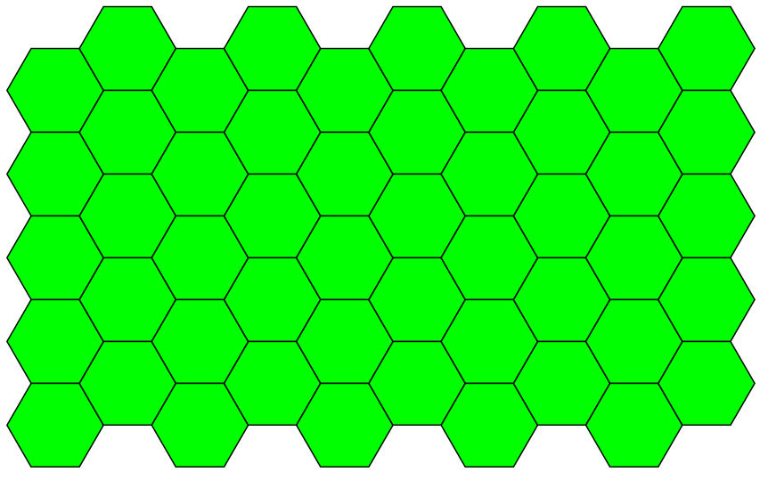
In this study we will adapt a a two dimensional square and hexagonal tilling as shown in Figure 1.
Figure 1. Hexagonal tiling.
3. Investigation of the movement with discrete time in two small cell complexes
Given a two-dimensional tessellated surface, we seek to investigate the movements of a molecule to neighboring cells via the cell walls from a given starting point. We will discuss the movement of the molecule with starting point at different cells in a \(2-D\) cell complexes specifically, square and hexagonal tiles.
3.1. Hexagonal tiling
Hexagonal tilling is the geometrical shape with six sides. Modeling the movement of the molecule on a hexagonal tiles requires a knowledge of the possible movements of the particle from the starting point. There are two possible starting points on a hexagonal tilling namely, from the center and at any of the border cell. When a molecule starts from the central cell, there are six possible movements via the cell wall. The probability \(p\) of the molecule to moves to a neighboring cell remains same as the same as the probability of throwing a fair die once. However, when a molecule starts from any the border cell, the there are only three possible movements at step one.
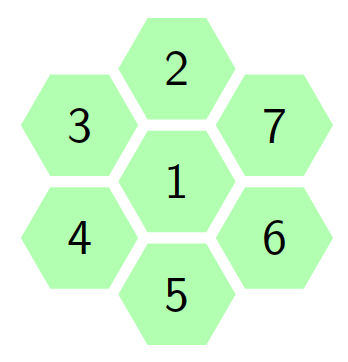
For small cell complex, the states are non-absorbing since the molecule cannot return to its starting point. The movements in a small cell complex is also considered irreducible Markov chain because it is possible for the biological molecule to move from one state to another. Let \(S={1,2,3,4,5,…m}\) represents the set of state space and \(n\) represent the number of steps the molecule takes to moves via the cell walls from the starting cell. At the rest \((n=0)\), the particle is at its starting state hence, the probability of the particle toward the neighboring cells is zero, i.e. \(p=0\). At the first step \((n=1)\), the particles moves to one of the neighboring tiles with probability \(p\). The Figure 2 portray the structure of the hexagonal tiling for the movement of the particle at \(n=1\) with the initial cell at the center, that is cell \(1\).
Figure 2. Hexagonal tiling under small cell complex.
From Figure 2 we are going to construct a transition matrix with \(7\) states as follows:
The probability of the particle to move from one cell to the nearest cell is \(p\). The total sum of probability to move from one cell to the neighbouring cells at step \(1\) is \(1\). Therefore, fore instance when the particle is initially at the central cell, then the probability of the particle to be in the same cell at step one is \(1-6p\) since the total probability add to one.
If the condition of symmetries exist, then \(P(i,j)=P(j,i)\). Now let \(A\) be the transition matrix of this behavior. So matrix \(A\) is as follow:
\begin{gather}
A=
\begin{bmatrix}
1-6p & p & p & p & p & p & p & \\ p& 1-3p & p & 0 & 0 & 0 & p &\\ p & p & 1-3p & p & 0 & 0 & 0 & \\ p & 0 & p & 1-3p & p & 0 & 0 & \\ p & 0 & 0 & p & 1-3p & p & 0 & \\ p& 0 & 0 & 0 & p & 1-3p & p &\\ p & p & 0 & 0 & 0 & p & 1-3p & \\
\end{bmatrix}
\label{9}
\end{gather}
(10)
3.2. Equilibrium status of the Hexagonal small cell complex
To derive the equilibrium status of the cell complex, we first require the notion of stationary distribution.
Using the transition matrix \(A\) given in Equation (10) to Equation (4), we have the following system of equations:
Theorem 10.
A Markov chain with a symmetric transition matrix P has a uniform stationary distribution \(1/n\), where
n is the number of states.
3.3. Calculation of Expected First passage time and Recurrence time in Hexagonal cell complex
Let \(T_{j1}\) be the time of hitting state \(1\) while starting from state \(j\), \(P(T_{j1}=n)\) for any \(j>1\) be the probability of the particle to hits state \(1\) from state \(j>1\) in \(n-\)steps and \(P_{ij}\) be the entries of the transition matrix \(A\) as shown in Equation (10). We are going to derive \(P(T_{j1}=n)\) with different values of \(n\) and \(j>1\). From Equation (7), we have:
Because of the symmetries in the small cell complex, we are going to derive only \( P(T_{21} = n)\), because \(P(T_{j1} = n) =P(T_{21} = n)\) for all \(j>=2\). Which means that the number of possible moves at step one when the particle is initially at one of the border cells is the same.
From Equation (16), when \(k={1,2,3\cdots m}\), we have the following equation:
Equation (19) implies that the probability of the particle to be in state \(1\) from state \(2\) at step one depends the value of the probability parameter \(p\).
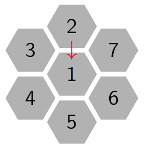
Figure 3 shows the movement of the molecule from state \(2\) to \(1\) in one step, \(n=1\). An arrow means the molecule move from state \(2\) to \(1\) with probability \(p\). The same applies to state \(3\), \(4\), \(5\), \(6\) and \(7\) to state \(1\).
Figure 3. Hexagonal tiling in small complex to show the movement of the particle from state \(2\) to \(1\) at step one.
Generally at any step \(n\), \(P(T_{j1}=n)\) for \(j>1\) and \(n\in \mathbb{N}\) is given by the following equation:
One can easily proof Equation (20) by Mathematical induction.
Equation (20) is very useful in calculating the expected passage time \(T_{ji}\) from state \(j\) to \(i\) with the help of Equation (8) as follows: From Equation (8), we deduce that
From the concept of derivatives, we have that if \(f(x)\) is a function defined by \(f(x)=x^{n}\) then derivative of \(f(x)\) is defined as \(\frac{d(f(x))}{dx}=nx^{n-1}\). Using this idea to Equation (22) lead to:
From Equation (24), we observe that the expected recurrence time to state \(1\) is \(7\). This means that the expected recurrence time \(T^{*}_{11}\) does not depend on the value of the probability parameter \(p\). Whether \(p\) is large or small, the expected recurrence time remain the same. This because of the fact that the Markov chains defined under hexagonal tiling is the finite Markov chain with single recurrence class. In this case we define a unique stationary distribution \(\pi_{i} =\frac{1}{\mu_{ii}}\), where \(\mu_{ii}\) is the expected recurrence time to state \(i\). Since the stationary distribution is unique it imply that the expected recurrence time is also unique.
3.4. Visualization of the transitional probabilities of transition matrix against time
In this part we are going to plot graphs of transitional probabilities against time with different values of the probability parameter \(p\) in transition matrix \(A\).
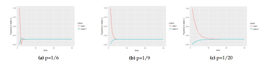
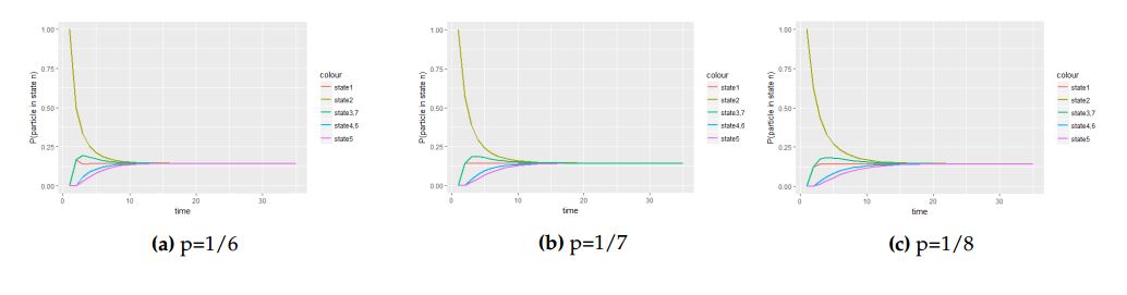
The following figures depict graphs of transitional probabilities against time when the particle is initially at the central cell with probability vector \(P^{0}_{1}=(1,0,0,0,0,0,0)\).
Figure 4. The panel of graphs to represent transitional probabilities against time interval of a transition matrix \(A\) with starting point at the central cell with with initial probability vector \(P^{0}_{1}=(1,0,0,0,0,0,0)\). From these figures state \(2\), \(3\), \(4\), \(5\), \(6\) and \(7\) overlap because they have the same stochastic behavior to the process.
From Figure 4 we saw how different values of the probability parameter \(p\) affect the attainment of the equilibrium status of the Markov process when the molecule is initially at the central cell.
3.4.1. When a particle is initially at one of the border cells
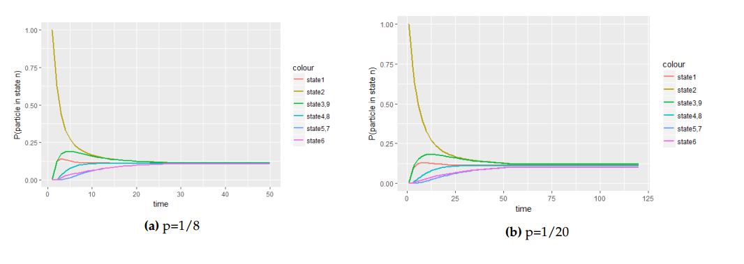
Now we are going to see how will the equilibrium be attained when the molecule is initially at one of the border cells with the initial probability vector \(P^{0}_{2}=(0,1,0,0,0,0,0)\) with different values of the probability parameter \(p\) as in Figure 4.
Figure 5. The panel of graphs to represent transitional probabilities against time interval of a transition matrix \(A\) with starting point at one of the border cells with with initial probability vector \(P^{0}_{2}=(0,1,0,0,0,0,0)\). With these graphs state \(3\) and \(7\) form one state while state \(4\) and \(6\) form a new state by overlapping because they have the same stochastic behavior to the process.
With Figure 4 and Figure 5, we deduce that when the molecule is initially at the central cell, the number of steps the process take to be in equilibrium is fewer than the number of steps the process take to attain equilibrium when the molecule is initially at one of the border cell.
Another way to investigate the fastness of the process toward equilibrium graphically is by using the log scale as shown in figures below.
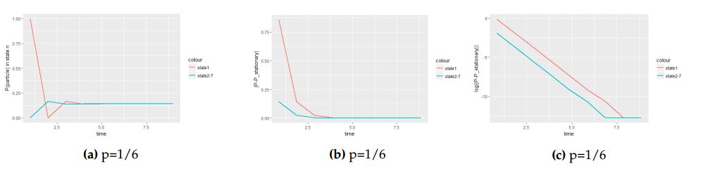
Figure 6. A panel of graphs to show how fast the equilibrium is attained in log scale under hexagonal tiling when the particle is initially at the central cell with probability vector \(v=(1,0,0,0,0,0,0)\).
Figure 6 show how the equilibrium is attained when the particle is initially at the central cell. Figure 6(b) show the difference between the process and the equilibrium distribution. And lastly Figure 6(c) depict how the steepness of the slope influence the attainment of stationary distribution.
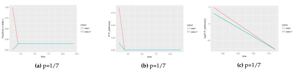
3.4.2. The use of log scale when the probability parameter \(p=\frac{1}{7}\)
We are to see how the value of the probability parameter \(p\) affect the slope in log scale toward attainment of equilibrium distribution.
Figure 7 is the continuation of Figure 6 but now with the probability parameter \(p=\frac{1}{7}\). The only different between Figure 7 and 6 is the time the process takes to attain equilibrium. The slope of Figure 7(c) is slight gently compared to the slope of Figure 6(c) which is much steeper indicate the fastness of the particle. In both cases the particle is initially at the central cell.
Figure 7. A panel of graphs to show how fast the equilibrium is attained in log scale under hexagonal tiling when the particle is initially at the central with probability vector \(v=(1,0,0,0,0,0,0)\).
Generally, we observe that the position of the particle initially and the value probability parameter \(p\) have direct consequences on the movement of the particle under hexagonal small cell complex as seen in Figures 6 and 7.
3.5. Square tiling
A square tile is a geometrical shape with four sides. Under this tilling, the possible movements of a biological cell depends on the location of the starting cell. When the starting cell is the central cell, then the biological molecules has has four possible movements away from the starting cell, which are North, South, East and East. Secondly, when the starting cell is one of the border cells at the corner then there are only two possible movements at step one; that is left/right and downward/upward movements. Thirdly, if the starting cell is one of the cells located at either North, South, East or West of the central cell, then there are only three possible movements of the molecule away from cell one; which are left/right, upward and downward movement.
Let \(S={1,2,3,4,5,…m}\) be the set of state space, and \(n\) represent the number of steps the biological cell takes to moves via the cell walls from the initial point. At \(n=0\), it means that no movement occurred, so the particle is still at the initial cell. So the probability of the movement to either of the neighboring cells is \(p=0\). Let \((X_{t}, t=0,1,2,3,…..n)\) be the stochastic process with Markov property, and let \(i\) and \(j\) be the current and next states respectively. At \(n=1\), the particle moves to one of the neighboring cells with probability \(p\). The figure below delineate the structure of the square tiling at \(n=1\).
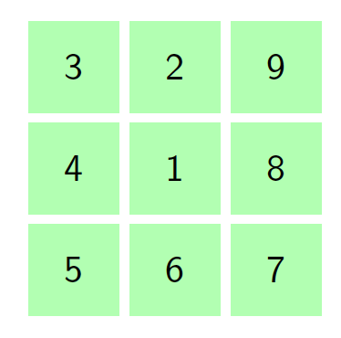
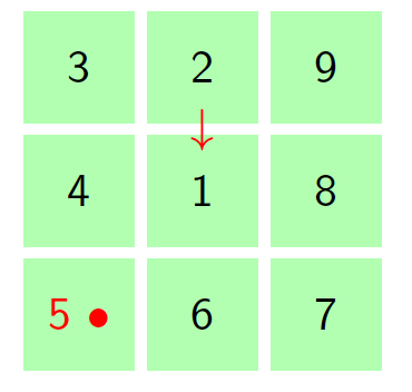
Figure 8. Square tiling in small complex with starting point at the central cell.
From Figure 8 we will construct a transition matrix with \(9\) states such that if the condition of symmetries exist, then \(P(i,j)=P(j,i)\). At step \(1\), when the particle is initially at the central cell, then it can only moves to cell \(2\), \(4\), \(6\) and \(8\) with probability \(p\) to each cell, then the probability of the particle to be in cell one at step \(1\) is \(1-4p\) since the total probability add to \(1\). Now let \(P\) be the transition matrix of this behavior with initial vector \(P^{0}_{1}=(1,0,0,0,0,0,0,0,0)\). So matrix \(P\) is as follow:
\begin{gather}
P=
\begin{bmatrix}
1-4p & p & 0 & p & 0 & p & 0 & p & 0 & \\ p& 1-3p & p & 0 & 0 & 0 & 0 & 0 & p &\\ 0 & p & 1-2p & p & 0 & 0 & 0 & 0 & 0 & \\ p & 0 & p & 1-3p & p & 0 & 0 & 0 & 0 & \\ 0 & 0 & 0 & p & 1-2p & p & 0 & 0 & 0 & \\ p& 0 & 0 & 0 & p & 1-3p & p & 0 & 0 &\\ 0 & 0 & 0 & 0 & 0 & p & 1-2p & p & 0 & \\ p & 0 & 0 & 0 & 0 & 0 & p & 1-3p & p & \\ 0 & p & 0 & 0 & 0 & 0 & 0 & p & 1-2p & \\
\end{bmatrix}
\label{60}
\end{gather}
(28)
Since it possible to move from one state to another, then the transition matrix \(P\) defined in Equation (28) characterizes the irreducible Markov chain. state \(1\), \(2\), \(3\), \(4\), \(5\), \(6\), \(7\), \(8\) and \(9\) forms a closed recurrent class. The Markov chain defined in Equation (28) define aperiodic Markov chain. all states are non absorbing. Since transition matrix \(P\) define irreducible Markov chain, then it is also ergodic.
3.6. Equilibrium status of the square small cell complex
To determine the equilibrium status of the square small cell complex, we need to apprehend the worth of stationary distribution.
Since transition matrix \(P\) is the symmetric matrix, we are are going to apply the assertion of Theorem 10 to derive the equilibrium status of the square small cell complex. Theorem 10 argue that if \(P\) is the symmetric transition matrix then the stationary distribution is defined by \(1/n\), where \(n\) is the number of states. Therefore the stationary distribution is defined by the following equations:
3.7. Calculation of expected first passage time and recurrence time in square cell complex
As in hexagonal small cell complex, we are going to derive hitting time probabilities and expected passage time from one state to another in square cell complex.
Let \(T_{j1}\) be the time of hitting state \(1\) while starting from state \(j\), \(P(T_{j1}=n)\) for any \(j>1\) be the probability of the particle to hits state \(1\) from state \(j>1\) in \(n-\)steps and \(P_{ij}\) be the entries of the transition matrix \(P\) as shown in Equation (28).
We are going to derive \(P(T_{j1}=n)\) with different values of \(n\) and \(j>1\). Now using the idea of Equation (7), we have
Because of the symmetries in the small cell complex, we derive only \(P(T_{21} = n)\) and \( P(T_{51} = n)\), because \(P(T_{j1} = n) =P(T_{21} = n)\) for \(j=(4,6,8)\) and \(P(T_{j1} = n) =P(T_{51} = n)\) for \(j=(3,7,9)\), because of having the same stochastic behavior to the Markov process at step one. Using \(j=(2,5)\) into Equation (34) with \(P_{ij}\) from Equation (28), we have
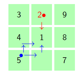
Figure 9 shows the movement of the molecule in a square cell complex from state \(j>1\) to state \(1\). The red bullet (dots) represent the zero probability of the movement of the particle from the respective states with red dots to state \(1\) at step one. The arrow lines represents the probability \(p\) of the molecule to move from the respective particle to state \(1\) at \(n=1\). There is only one path to the central cell at step one.
Figure 9. Square tiling in small cell complex to depict the movement of the particle from state \(j>1\) to state \(1\) in one step.
For \((n=2)\), Equation (27) lead to:
Using \(P_{ij}\) from Equation (28) into Equation (38), With the fact that \(P_{24}=P_{26}=P_{52}=P_{28}=P_{58}=0\) because at one step there is no transition to the respective states, gives:
Figure 10 delineate the movement of the molecule from state \(j>1\) to state \(1\) at \(n=2\). When the molecule at step \(1\) is at either state \(2\), \(4\), \(6\) or \(8\), then it will move to state \(1\) means that at step \(2\) there will be no movement of the particle from the respective states to state \(1\). Conversely, when the particle is at either \(3\), \(5\), \(7\) or \(9\), then at step \(1\) the molecule will not move to state \(1\). However, at step \(2\) the molecule will move to state \(1\) via the neighboring states.
Figure 10. Square tiling in small complex two depict the movement of the particle from state \(j>1\) to state \(1\) in two steps.
For \((n=3)\), Equation (32) reduces to:
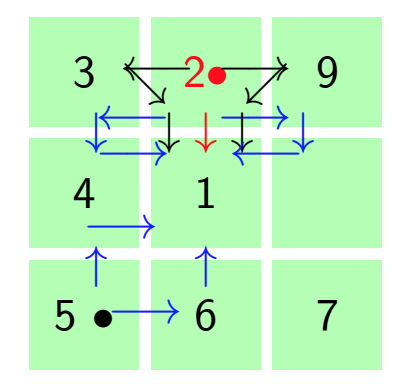
Figure 11 render the movement of the biological molecule from sate \(j>1\) to state \(1\) in three steps. In this figure we will show the movements of the particle from state \(j>1\) to state \(1\) in two circumstances with \(n=3\). First, when the molecule is at one of the corner cells and second, when the molecule is at one of the up/down/left/right cells.
Figure 11. square tiling in small complex two depict the movement of the particle from state \(j>1\) to state \(1\) in three steps.
When the molecule is initially at one of the corner cells, then at step one the molecule will not move to state \(1\) but it can move to either of the neighboring cells. In this context, the molecule will be in state \(1\) after two steps. Contrary, when the molecule is initially at one of the sides cell other the corner cells, then at step \(1\) it is possible for the molecule to move to state one directly. It can first move to one of the other neighboring cells then at \(n=2\) it can either moves to the neighbor cell of the current or move back to initial cell and finally at \(n=3\) it moves to state \(1\).
3.7.1. Calculation of the expected passage time under small cell complex in square tiling
To calculate the first passage time \(T_{j1}\), we follow the following procedures with reference to Equation (9) and transition matrix in Equation (28). The expected passage time from state \(j>1\) to state \(1\) is given by:
From the result of Equation (50), we observe that the expected recurrence time to state \(1\) is \(9\). This means that the expected recurrence time \(T^{*}_{11}\) does not depend on the value of the probability parameter \(p\).
3.8. Visualization transitional probabilities against time interval of transition matrix \(P\) under square small cell complex
Under square small cell complex we have three different types of non equivalents cell which are:
Cell complex with starting point at the central cell, with initial vector \(P^{0}_1 = (1, 0, 0, 0, 0,0, 0, 0, 0)\).
Cell complex with starting point at the corner border cell,with initial vector \(P^{0}_3 = (0, 1, 0, 0, 0,0, 0, 0, 0)\).
Cell complex with the starting point at the sides cells, that is North-South and South-East of the central cell,with initial vector \(P^{0}_3 = (0, 0, 1, 0, 0,0, 0, 0, 0)\).
We will show different graphs of transitional probabilities against time with different values of the probability parameter \(p\) in transition matrix \(P\). Figure 12 shows the transitional probabilities against time when the particle is initially at the central cell with probability vector \(P^{0}_{1}=(1,0,0,0,0,0,0)\).
Figure 12. The panel of graphs to represent transitional probabilities against time interval of a transition matrix \(P\) with starting point at the central cell with with initial probability vector \(P^{0}_{1}=(1,0,0,0,0,0,0,0,0)\). From these figures state \(2\), \(4\), \(6\), and \(8\) overlap to form a new state while state \(3\), \(5\), \(7\) and \(9\) overlap because they have the same stochastic behavior to the process.
In Figure 12 we observed the behavior of the process when the particle is initially at the central cell with different values of the probability parameter \(p\). We will now explore how different values of the probability parameter alter the process when the molecule is initially at one of the corner border cells. When the particle is initially at one of the corner border cells with probability vector \(P^{0}_2 = (0, 1, 0, 0, 0,0, 0, 0, 0)\), we have the following figures.
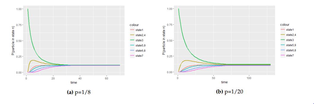
Figure 13. The panel of graphs to represent transitional probabilities against time interval of a transition matrix \(P\) with starting point at the one of the border corner cell with with initial probability vector \(P^{0}_{2}=(0,1,0,0,0,0,0,0,0)\). From these figures state \(3\) and \(9\), \(4\)and \(8\), \(5\) and \(7\) overlaps together to form new states respectively because they have the same stochastic behavior to the process.
Another non equivalent cell in square cell complex is when the particle is initially at one of the side cells, that is North-South and South-East of the central cell with initial probability vector \(P^{0}_{3}=(0,0,1,0,0,0,0,0,0)\).
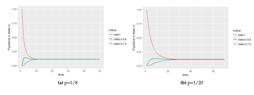
From Figure 14 below, we observe that the equilibrium is attained faster with larger values of the probability parameter \(p\) compared to small values of the probability parameter \(p\). This is justified with comparison of the number of steps taken by the process to be in equilibrium in 14(a) with the number of steps the process take to attain in equilibrium in 14(b). In Figure 14(b) the process takes a number of steps to be equilibrium which means that the molecule is slow when the probability parameter \(p\) is small. With this fact we deduce that the movement of the molecule is faster when the value of the probability parameter \(p\) is large and slower when the value of the probability parameter \(p\) is small.
Figure 14. The panel of graphs to represent transitional probabilities against time interval of a transition matrix \(P\) with starting point at the one of the side cells, that is North-South or East-West of the central cell with with initial probability vector \(P^{0}_{3}=(0,0,1,0,0,0,0,0,0)\). From these figures state \(2\) and \(4\), \(5\)and \(9\), \(6\) and \(8\) overlaps together to form new states respectively because they have the same stochastic behavior to the process.
With these three non equivalent cells in square small cell complex we deduce that the molecule attain equilibrium faster when the particle is initially at the central cell because of the possible number of moves at the first step. This means that the number of possible cells to be visited when the particle is
initially at the central cell is large compared to when the particle is initially at one of the border cell.
3.9. \(n\)-step transition matrix
From Equation (2), we have that:
$$ P(X_{t+1} = j / X_{t} = i ,X_{t-1} = i-1,X_{t-2} = i-2, . . . ) = P(X_{t+1} = j / X_{t} = i)=P(i , j ),$$
where \(P(i , j )\) define the probability of the biological molecule to move from state \(i\) to state \(j\) at step one. At step \(2\), the transitional probabilities of the biological molecule to be in state \(j\) given that \(i\) is the initial state is obtained by taking the summation of the products of probabilities from state \(i\) to state \(k\) with probabilities from State \(k\) to \(j\) where \(k\) is an intermediate stop between \(i\) and \(j\).
Let \(n\) be the number of steps that the molecule pass from state \(i\) to state \(j\), then the transitional probabilities \(P(i , j )\) from state \(i\) to state \(j\) at \(n-\)steps denoted by \(P^{n}_{ij}\) can be deduced from the Chapman-Kolmogorov equation in theorem. The collection of the transitional probabilities obtained here form the elements of the transition matrix of the Markov chain. Suppose that \(K\) is the transition matrix defined at \(n=1\), then at \(2-\)steps then the \(3-\)steps transition matrix is defined by \(K^{3}\). We can define the \(n-\)steps transition matrix as \(K^{n}\), where \(K^{n}\) represents the multiplication of the matrix \(K\) itself \(n-\)times. For our case we have transition matrices \(P\) and \(A\) that describes the movement of the biological molecules at small cell complex in square and hexagonal tiling respectively. By taking transition matrix \(P\) as the reference matrix, we will derive the two step transition matrix denoted by \(P^{2}\).
Let \(P_{ik}\) be the probability of the biological molecule to be in an intermediate stop \(k\) from state \(i\) , \(P_{kj}\) be the probability of the particle to be in state \(j\) from an intermediate stop \(k\) and \(M\) be the number state states then
The computation continues up to \(n-\)steps transitional probabilities \(P^{n}_{ij}\) of the \(n-\)steps transition matrix, with \((n)\) being the maximum number of steps. The following general formula guide on how to obtain the entries of the \(n-\)steps transition matrix \(P^{n}\).
Equation (54) represent the \(n-\)steps transitional matrix of the Markov chain.
From Equation (52) and Equation (54) we observe that \(P^{n}_{ij}\) is the result of the products of transitional matrices. Without loss of generality and by avoiding tedious computations with Chapman-Kolmogorov Equation; we simply apply the matrix multiplication to the \(n^{th}-\)power to obtain the \(n-\)steps transition matrix. Therefore the \(n-\)step transition matrices for our transition matrices \(P\) and \(A\) are defined by \(P^{n}\) and \(A^{n}\) .
3.10. Lumpability of the Markov chain Under small cell complex
Theorem 8 argue that if a Markov chain \({X_t}, t\in T\) where \(T\geq0\) can be portioned into sub-process of which every process retains the Markov property, then the Markov chain \({X_t}, t\in T\) where \(T\geq0\) is Lumpable. The main idea of Lumpability of the Markov chain is for Aggregation of the Markov chain to reduce the number of state space while maintaining the Markov property.
By using the assertion of Theorem 8, we can make aggregation of the Markov chain by reducing the number of state space in the respective transition matrices \(P\) and \(A\). Lets see the aggregation of the transition matrix \(A\) with the aid of Figure 2 and the assertion of Theorem 8 by symmetries. Let \(C\) denotes the central cell and \(B\) denotes border cells of the hexagonal tiling in Equation (10). Since all the border cells are symmetric then we can define \(B’\) as the new state formed by aggregation of all the border cells. Using this idea, we consider the group \(G\) of the state symmetries of the transition matrix \(A\) with the structure of symmetric of the regular hexagon(Dihedral group of \(D_6\)) generated by the following permutation, \(\rho_1=(1)(234567)\). Where \((1)\) stand for \(C’\) and \((2,3,4,5,6,7)\) represent state \(B’\) formed by aggregation. This means that the original Markov process \(X_{t}\) is lumpable with respect to the permutation \(\rho_1=(1)(234567)\) and the partition \(C_{1}=\{\{1\},\{2,3,4,5,6,7\}\}\) . The new aggregated Markov process \(X’_{t}\) preserve the Markov property.
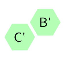
Figure 15 depict the new transition matrix \(A’\) formed as the aggregation of state symmetries of transition matrix \(A\).
Figure 15. Hexagonal tiling in small complex formed as the result of aggregation symmetric states.
Now we are going to see how the transition matrix \(A’\) looks as the result of permutation \(\rho_1=(1)(234567)\) with starting vectors \(v’=(1,0)\). Vector \(v’\) is the result of the aggregation of the initial vector \(v=(1,0,0,0,0,0,0)\) and \(\rho_1\) is the permutation of the state symmetries of the original Markov chain.
Definition 11.
A chain \(X’_t\) is said to be a trivial aggregated chain if \(X’_t\) is the aggregated chain for the Markov chain \(X_t\) and initial distribution \(\pi\), where \(\pi\) is a vector of finite probabilities [14]
To get the transition matrix \(A’\), we use the idea of lumpability to the transition matrix \(A\) defined in Equation \eqref{9}. Since state \(1\), \(2\), \(3\), \(4\), \(5\), \(6\) and \(7\) are symmetrically equivalent, then we are going to combine them together by aggregation of symmetric states. The new transition matrix \(A’\) is defined as follows:
To obtain \(a’_{ij}\) we apply aggregation of the Markov chain for the states with same stochastic behavior to the process. That means that the permutations or reordering of their states probabilities are the same. With the help of \(P_{ij}\) from Equation (10), \(a’_{ij}\) from Equation (55) are defined as follows:
Using this result we are going to solve the equilibrium status of the cell complex under a new transition matrix \(A’\). Since the transition matrix has only two states, then the new normalization equation is given by:
For \(p\ne0\), we append Equation (58) to Equation (60) and then obtaining the solution of the equilibrium status as:
3.10.1. Calculation of the expected passage time and recurrence time under symmetries in Hexagonal tiling
Using the aggregated Markov process we will examine how the transitional probabilities looks like as the result of aggregation of state symmetries. Let \(T_{B’C’}\) be the time of hitting state \(C’\) while starting from state \(B’\), \(P(T_{B’C’}=n)\) be the probability of the molecule to hits cell \(C’\) from cell \(B’\) in \(n-\)steps and \(P_{B’C’}\) be the entries of the transition matrix \(A’\) as shown in Equation (57). We will derive \(P(T_{B’C’}=n)=f^{n}_{B’C’}\) with different values of \(n\). Now using the idea of Equation (7), we have
Now at \(n-\)steps, the results from Equation (64) and Equation (65) give the general form of the probability of the molecule to be in state \(C’\) from state \(B’\) at \(n-\)steps as:
3.10.2. Calculation of expected passage time from state B’ to C’
To compute the expected passage time from state \(B’\) to \(C’\) from the the cell complex defined in Figure 15 we use the following statistical formula:
3.10.3. State symmetry under hexagonal small cell complex
For Square tiling we have three non equivalent cells \(A’\), \(B’\) and \(C’\), that is the central cell, corner cells and sides cells. Using this idea we will generate the group of symmetries with the aid of Theorem 8. Now using the transition matrix \(P\) in Equation (28), we can generate the group of symmetries of the square, that is Dihedral group \(D_4\), [1]. By using Figure 8 and transition matrix \(P\) in Equation (28) with the initial vector \(P^{0}_{1}=(1,0,0,0,0,0,0,0,0)\), we can generate a group \(G\) of state symmetries of the \(P\) generated by the following permutations, \(\rho _1=(1)(2468)(3579)\). So the Markov chain \(X_{t}\) is lumpable with the partition \(C=\{\{1\},\{2,4,6,8\},\{3,5,7,9\}\}\) and the initial vector \(v=(1,0,0)\).
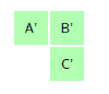
The Figure 16 below shows the structure of the tiling formed after aggregation.
Figure 16. Square tiling in small complex with starting point at the centre cell after aggregation.
The new transition matrix \(P’\) is defined as follows:
The transition matrix \(P’\) in Equation (72) is of size \(3\times 3\) which make numerical and algebraic computations a bit less tedious compared to the original transition matrix of size \(9\times 9\). Using this result we are going to solve the equilibrium status of the cell complex under a new transition matrix \(P’\). From Equation (4), we have that \(\pi=\pi P\). By using transition matrix \(P’\) in Equation (72) into Equation (4) we have the following system of equations:
To solve Equation (74), when \(p\ne0\) we append the normalization vector equation \(\pi\), as \(\pi _{1}+\pi _{2}+\pi _{3}=1\) to Equation (74) to get the solution as:
3.10.4. Calculation of the expected passage time and recurrence time under symmetries in square tiling
Using the transition matrix \(P’\) generated after the aggregation of the Markov chain, we are going to see how the hitting time probabilities and expected passage time behave. Let \(A’\), \(B’\) and \(C’\) denotes the states of the new transition matrix formed after aggregation. Where \(A’\) represent the corner cell, \(B’\) denotes the sides cell while \(C’\) represent the central cell. Let \(P(T_jC’=n)\) for \(j=(A’,B’)\) denotes the probability of the molecule to move from state \(j=(A’,B’)\) to state \(C’\) in \(n-\)steps.
Using the idea of Equation (7), we have
An advantage of performing aggregation of the Markov chain is that it make numerical and algebraic computations easy by reducing the size of the transition matrix.
4. Results from numerical simulation
Under this research numerical simulation has been carried out as the way of verifying some of the algebraic results and deduce some of the results which are not easy to deduce analytically in both small cell complexes. The Table 1 show how different values of the probability parameter \(p\) affect the expected passage time from one state to another under hexagonal small cell complex.
Table 1. A table to represent the effect of changing the value of parameter \(p\) on expected passage time from one state to another under square small cell complex.
start state
end state
p
expected passage time
2
1
0.1667
6.01
1
2
0.1667
12.95
2
5
0.1667
16.65
5
2
0.1667
16.54
2
1
0.1
10.04
1
2
0.1
21.46
2
5
0.1
28.17
5
2
0.1
27.97
2
1
0.001
100.86
1
2
0.001
213.04
2
5
0.001
283.43
5
2
0.001
279.47
The Table 2 show how different values of the probability parameter \(p\) affect the expected passage time from one state to another under square small cell complex.
Table 2. A table to represent the effect of changing the value of parameter \(p\) on expected passage time from one state to another under square small cell complex.
start state
end state
p
expected passage time
2
1
0.25
8.27
1
2
0.25
13.00
3
1
0.25
10.01
1
3
0.25
21.13
2
1
0.1
19.84
1
2
0.1
32.52
3
1
0.1
24.88
1
3
0.1
54.38
2
1
0.001
199.72
1
2
0.001
323.69
3
1
0.001
250.52
1
3
0.001
536.33
With algebraic computations we observed that different values of the probability parameter \(p\) has no effect on the expected recurrence time. The Table 3 show the numerical simulated results to verify algebraic computations of expected recurrence time.
Table 3. A table to represent to display expected recurrence time under hexagonal and square tiling with different values of \(p\).
start state
end state
p
ERH
ERS
1
1
0.1667
7.09
9.03
1
1
0.25
7.01
9.05
1
1
0.1
7.03
8.85
2
2
0.1
6.89
8.66
7
7
0.1
7.01
8.54
1
1
0.001
7.39
9.16
3
3
0.001
6.7
8.83
The results of Table 1, 2 and 3 are very important in verification of algebraic computations. For instance from Equation (23), we have that the expected passage time from state \(j>1\) to state \(1\) is given by \(T_{j1}=1/p\). We are going to use the results of Table 1 to verify this result as follows:
From Table 1, we have that with \(p=0.1\) the expected passage time from state \(2\) to \(1\) is \(10.04\). If we use \(p=0.1\) to Equation (23), we have that \(T_{j1}=10\) which is not so much different with the numerical results, which means that algebraic computations of expected passage time under hexagonal tiling are correct.
We can verify the algebraic results of Equation (47) from numerical results presented in Table 2. From Table 2, we have that the expected passage time from state \(2\) to \(1\) with \(p=0.25\) is \(8.27\), and from Equation (47), we have that \(T_{21}=2/p\). With \(p=0.25\), \(T_{21}=8\) which is almost the same with the numerical results. One can also verify numerical results for recurrence time using Table 3.
4.1. Comparison of both tiling
Under small cell complex, with the aids of graphs of probability against time, we recognize that the movement of a molecule in hexagonal tilling is faster than in square tilling. This is because the attainment of stationary distribution in hexagonal tilling takes few steps as compared to the number of steps that the molecule takes to be in equilibrium in square tiling. For example in Figure 4(f) that depict the movement in hexagonal tiling with the value of the probability parameter \(p=\frac{1}{20}\), the number steps to attains the equilibrium is less than \(15\) while in Figure 14(d) that shows the movement in square tiling with the same probability parameter \(p=\frac{1}{20}\), the number of steps that the process take to attain equilibrium status is more than \(20\).
Using the idea of expected passage time and recurrence time, we observe that in Hexagonal tiling the expected passage time from one state to another is small compared to the one needed in square tilling. And the expected time for the first return to the same state in Hexagonal tilling is slightly smaller than the one in Square tilling. For example in Equation (23), we observe that expected passage time is small compared to the one in Equation (47) and the same to the recurrence time in Equation (27) is smaller than the one in Equation (50).
Generally the movement of the particle under hexagonal tiling is seem to be faster than the movement of the particle under square tiling because at step one, the possible number of possible cells the particle can move to under hexagonal is six compared to four under square tiling. Which implies that the movement of the particle under hexagonal covers many cells within few steps than under square tiling.
5. Discussion of the investigations
Under this section we are going to discus various results that are obtained both numerically and analytically under hexagonal and square small cell complexes.
5.1. Impact of changing the value of probability parameter \(p\) toward attainment of stationary distribution.
We discovered that changing the value of the probability parameter \(p\) has a direct impact on the movement of the molecule over the cell complex in attainment of equilibrium status. With this essay we observed that when the probability parameter \(p\) is large then the process is likely to attain equilibrium faster than when \(p\) is small. If we refer to Figures 4(a) and 4(c) of which both display plots of probabilities against time under hexagonal tiling, we observe that the time taken for the process to be in equilibrium status under 4(a) is smaller compared to the time in Figure 4(f). This is due to the variation of the value of the probability parameter used in both cases. The case is the same for square tiling.
5.2. Impact of the parameter \(p\) in numerical simulation
With the aid of numerical simulation, the value of \(p\) has the direct impacts on the number of transits for the molecule to move from one state to another. When the probability parameter \(p\) is small, the number of moves to the next state is large unlike to when \(p\) is large.
5.3. Changing the value of parameter \(p\) in numerical simulation under hexagonal tiling
Table 1 show how the value of the probability parameter \(p\) affect the movement of the particle from different state to the neighboring state. From Table 1 we observed that when the probability parameter \(p\) is small then expected number of transition from one state to another is high compared to the large value \(p\). This is because when \(p\) is small then the movement of the molecule is slow unlike when \(p\) is large. Direct from Table 1 we observe that the expected number of transition from state \(2\) to state \(1\) is not equal to the expected number of transition from state \(1\) to \(2\), this might be because of the different paths a molecule use while in movement.
5.4. Changing the value of parameter \(p\) in numerical simulation under square tiling
Under simulation of hitting time in square small cell complex the value of the probability parameter \(p\) has direct impacts on the number of transitions from one state to to another state. As in hexagonal small cell complex different values of the probability \(p\) alter the speed of the molecule while in motion. In this case the smaller the value of the probability parameter \(p\), the larger the expected number of transitions and vice versa.
Table 2 show how different values of the probability parameter \(p\) affect the expected passage time from one state to another state.
From Table 2 , we observe that as the probability parameter \(p\) decreases, the number of transitions that are expected for the particle to be at a certain from the initial defined state increases. With this fact we deduce that the probability parameter \(p\) is inversely proportional to the number of transitions.
5.5. Numerical simulation of expected recurrence time with different values of the probability parameter \(p\)
With algebraic computations we observed that the expected number of transitions for the first return to the same state, that is expected recurrence time to state \(1\) is \(7\) for hexagonal tiling and \(9\) for square small cell complexes as defined in Equation (27) and Equation (50) respectively.
Table 3 render the expected recurrence time with different values of the parameter \(p\) in both hexagonal and square small cell complex, which has no visible different with the one defined in Equation (27) and Equation (50).
5.6. Expected passage time from state \(i\) to \(j\) and from state \(j\) to \(i\) with relation to symmetries
Basing on the results from numerical simulation, we observed that when two states \(i\) and \(j\) are symmetric, that is they have the same stochastic behavior to the process then the expected passage time from state \(i\) to state \(j\) is the the same as the expected passage time from state \(j\) to state \(i\). But if state \(i\) and \(j\) are non equivalents states then the expected passage time from state \(i\) to \(j\) is not equal to the expected passage time from state \(j\) to state \(i\). The reason behind the differences is that that when two states \(i\) and \(j\) have the same stochastic behavior to the process then their paths are likely to be similar, but if \(i\) and \(j\) are non equivalent states then their paths are not the same.
5.7. Comparison of results from numerical simulation with results from algebraic computations.
This essay comprise algebraic computation and numerical simulation. The purpose of numerical simulation is to verify algebraic computation. With numerical simulation we generated some results that are useful in testing whether algebraic results are correct . For example the expected passage time under hexagonal tiling as defined in Equation (23) can be verified by complementing it with the results from numerical simulation defined in Table 1. The results depicted in Table 1 with different values of the probability parameter \(p\) approximate the expected passage time defined in Equation (23). One can verify easily for square tiling.
5.8. Effect of changing the initial position of the molecule under small cell Complex.
Changing the starting point of the movement of the particle under small cell complex has direct impact on the movement of the molecule. One of the viable effect is the attainment of stationary distribution. By considering Figures 4 and 5 of which the starting point is the central cell and one of the border cells respectively, we observed that when the particle is initially at the central cell, then the stationary distribution is arrived faster as seen in Figure 4 than when molecule is at one of the border cells as portrayed in Figure 5. This is because when the molecule is initial at the central cell, that is cell \(1\) as in Figure 4, the probability of moving from state \(1\) to either of the other states is the same at step one, while when the particle is initially at one of the border cell it is not possible to visit to either of the other states at step one, means the probability is not the same. This means that when the particle is initially at the central cell, the are are numerous possible number of cells to be visited at step one compared to when the molecule is initially at one of the border cells. In this case the value of the probability parameter \(p\) is assumed to be constant. The same effect observed under square tiling.
5.9. Impact of the number cells in the cell complex for the molecule to return to the same state.
Under this study we observed that the number of cell within the respective cell complex has a direct impact on the expected recurrence time of the molecule. Basing on the results from this essay we realized that the expected recurrence time is equal to the number states or cells in the cell complex. To verify this we refer to algebraic results presented in Equation (27) and Equation (50) for hexagonal and square tiling respectively. Under hexagonal tiling we have \(7\) states and the expected recurrence time is \(7\) as in Equation (27), while in square tiling we have \(9\) states and the recurrence time is \(9\) as in Equation (50).
5.10. Effect of symmetries on the cell complex.
When the cell structure is large, algebraic calculations becomes tedious and cumbersome. In this essay we observed that aggregation of state symmetries is a very useful and meaningful technique to handle algebraic computations of the the Markov chain \(X_{t}\) with large state space \(S\). Aggregation of state symmetries of the Markov chain \(X_{t}\) reduced the difficulties and time for algebraic computations of various results. Among the impact of aggregation state symmetries in this essay are observed in Equation (72) and Equation (57) which are the new transitions matrix \(P’\) and \(A’\) of the original transition matrices \(P\) and \(A\) of square and hexagonal tiling respectively as defined in Equation (28) and Equation (10) respectively. Before aggregation of state symmetries of the transition matrices \(P\) and \(A\) as defined in Equation (28) and Equation(10) respectively, it was very difficult to derive the equilibrium status of the Markov process as defined in Equation (29) and Equation (14) respectively. But after obtaining the new transition matrices \(P’\) and \(A’\) as defined in Equation (72) and Equation (57) respectively; it became easier to arrive to equilibrium status as defined in Equation (75) and Equation (61) respectively.
6. Conclusion
At the end of this study we observed that the value of the probability parameter \(p\) has a big influence in the fastness of the molecule in both tilings. We observed when the value of the probability parameter \(p\) is small, the speed of the particle is very slow and vice versa. So the attainment of stationary distribution is affected with the value of the probability parameter \(p\), that is the larger the value of the probability parameter, the faster the equilibrium is achieved and vice versa. Another thing we noticed is that the value of the probability parameter has no effect on expected recurrence time. This means that regardless of the value of the probability parameter \(p\) the expected recurrence time always remains the same. We also observed that the position of the molecule at initial step has a big influence on the attainment of stationary distribution. With this study we noticed that when the molecule is initially at the central cell, then attainment of equilibrium is faster than when the particle is initially at one of the border cells. This is because the number of possible cells to be visited at the first step when the particle is initially at the central cell is large compared to when the particle is initially at one of the border cells. We also realized that the process is likely to attains equilibrium in hexagonal tiling than in square tiling due to the different in the number of state spaces and the possible cell to be visited when the particle is initially at the central cell.
This work was very interdisciplinary because many discipline of mathematics were employed for its completion. Among the discipline of mathematics employed in this essay are group theory, probability theory, differentiation of functions and linear algebra. In this work group theory was used to understand the concept of state symmetries and permutation. Linear algebra helped in the whole concept of matrices, vectors and solving the system of linear equations, differentiation helped in generalization some geometrical series while probability theory was useful in understanding stationary distribution.
Acknowledgments
The authors would like to express their thanks to the referee for his useful remarks.
Author Contributions
All authors contributed equally to the writing of this paper. All authors read and approved the final manuscript.
Competing Interests
The author(s) do not have any competing interests in the manuscript.
References
Ring, A. (2004). State symmetries in matrices and vectors on finite state spaces. arXiv preprint math/0409264.[Google Scholor]
Beneš, V. E. (1978). Reduction of network states under symmetries. Bell System Technical Journal, 57(1), 111-149. [Google Scholor]
Barr, D. R., & Thomas, M. U. (1977). An eigenvector condition for Markov chain lumpability. Operations Research, 25(6), 1028-1031.
[Google Scholor]
Karmanov, A. V., & Karmanova, L. A. (2005). Estimation of finite probabilities via aggregation of Markov chains. Automation and Remote Control, 66(10), 1640-1646. [Google Scholor]
Schweitzer, P. J. (1983, September). Aggregation methods for large Markov chains. In Proceedings of the International Workshop on Computer Performance and Reliability (pp. 275-286). North-Holland Publishing Co. [Google Scholor]
Sumita, U., & Rieders, M. (1989). Lumpability and time reversibility in the aggregation-disaggregation method for large Markov chains. Stochastic Models, 5(1), 63-81.[Google Scholor]
Ching, W. K., Huang, X., Ng, M. K., & Siu, T. K. (2013). Higher-order markov chains. In Markov Chains (pp. 141-176). Springer, Boston, MA. [Google Scholor]
Snodgrass, S., & Ontañón, S. (2014). Experiments in map generation using Markov chains. In FDG.[Google Scholor]
Snodgrass, S., & Ontañón, S. (2014, September). A hierarchical approach to generating maps using markov chains. In Tenth Artificial Intelligence and Interactive Digital Entertainment Conference. [Google Scholor]
Kayibi, K., Samee, U., Merajuddin, M., & Pirzada, S. (2019). Generalized Dominoes Tiling’S Markov Chain Mixes Fast. Journal of applied mathematics & informatics, 37(5-6), 469-480. [Google Scholor]
Kayibi, K. K., & Pirzada, S. (2018). T-tetrominoes tiling’s Markov chain mixes fast. Theoretical Computer Science, 714, 1-14.[Google Scholor]
Kayibi, K. K., & Pirzada, S. (2012). Planarity, symmetry and counting tilings. Graphs and Combinatorics, 28(4), 483-497. [Google Scholor]
Dyer, M., Kannan, R., & Mount, J. (1997). Sampling contingency tables. Random Structures & Algorithms, 10(4), 487-506. [Google Scholor]
Harris, T. E. (1952). First passage and recurrence distributions. Transactions of the American Mathematical Society, 73(3), 471-486.[Google Scholor]