
For an integer \(r\geq1\), let \([r]=\{1,\ldots,r\}\), with \([0]=\varnothing\). For \(m\geq1\) and \(n\geq0\), let \(G_{m,n}\) denote the rectangular grid graph with vertex set \(V(G_{m,n})=[m]\times[n]\), where \((i,j)\) and \((i’,j’)\) are adjacent if and only if \(\lvert i-i’\rvert+\lvert j-j’\rvert=1\). Thus, the vertices of \(G_{m,n}\) represent the cells of the grid, and graph adjacency corresponds to edge adjacency of cells.
A binary coloring of \(G_{m,n}\) is a map \(\pi:V(G_{m,n})\to\{0,1\}\), where \(0\) denotes white and \(1\) denotes black. We write \(\Omega_{m,n}:=\{0,1\}^{V(G_{m,n})}\) for the set of all such colorings. For \(\pi\in\Omega_{m,n}\), let \(c_w(\pi)\) and \(c_b(\pi)\) denote the numbers of connected components of the induced subgraphs \(G_{m,n}[\pi^{-1}(0)]\) and \(G_{m,n}[\pi^{-1}(1)]\), respectively, and set \(K(\pi):=c_w(\pi)+c_b(\pi)\).
When \(n=0\), the vertex set of \(G_{m,0}\) is empty and \(\Omega_{m,0}\) consists of a unique empty coloring, also denoted by \(\varnothing\). We adopt the convention \(c_w(\varnothing)=c_b(\varnothing)=K(\varnothing)=0\).
Our objective is to enumerate binary colorings according to the pair \((c_w,c_b)\) and, in particular, to study the total cluster count
Under the uniform measure on \(\Omega_{m,n}\), the expectation of a statistic \(X:\Omega_{m,n}\to\mathbb R\) is \(\mathbb E_{m,n}[X] :=2^{-mn}\sum\limits_{\pi\in\Omega_{m,n}}X(\pi)\). Consequently, \(\mathbb E_{m,n}[K]=2^{-mn}S_{m,n}\).
Counting monochromatic components in random binary colorings is naturally related to site percolation at parameter \(1/2\) and to the expected number of connected monochromatic regions. Richey [1] studied this probabilistic viewpoint, including fixed-width limits and the two-dimensional limiting density. For fixed height \(m\), Mansour [2] introduced a finite-automaton method based on continuation equivalence and a column-by-column scan, obtaining a Bell-type finiteness bound and exact formulas for \(m\leq3\).
Connectivity-state transfer matrices are also standard in Potts-model and percolation computations. The Fortuin–Kasteleyn representation provides the classical connectivity formulation for Potts-type models [3]. In planar strips, only noncrossing frontier partitions can occur, leading to Catalan-type transfer spaces; see, for example, Salas and Sokal [4]. Scullard and Jacobsen use the same planar-connectivity principle for transfer-matrix computations in bond and site percolation [5]. Related recent developments for loop and Potts models appear in [6,7]. Accordingly, no priority is claimed here for the general noncrossing principle.
The contributions of the present paper are specific to binary monochromatic-cluster enumeration. First, we formulate a complete bicromatic frontier invariant and prove that its full connectivity partition is noncrossing. We then distinguish the unrestricted, colorwise-noncrossing, and full-noncrossing ambient state spaces, determine their exact cardinalities, and identify the full-noncrossing count with the large Schröder numbers.
Second, we introduce the block-adjacency graph \(Q(\Pi)\). This graph is connected for every partition \(\Pi\), and every reachable frontier state induces a proper two-coloring of it. Consequently,
where \(b_m\) counts the noncrossing partitions whose block-adjacency graph is bipartite and \(R_m\) is the \(m\)-th large Schröder number.
For \(m=4\), exactly one of the \(14\) noncrossing partitions has a nonbipartite block-adjacency graph. The remaining \(13\) partitions admit two complementary proper block colorings and therefore yield at most \(26\) nonempty states. The explicit witnesses in Table 2 show that all of them are reachable. Hence,
Separately, an unfiltered breadth-first search generates the complete height-four labeled transition system directly from the one-column transition rule. From its exact transition certificate, independently verified by an exact-arithmetic package, we construct \(T_4(p,q)\) and derive a reduced rational generating function for \(S_{4,n}\), a closed formula, a minimal linear recurrence of order five, a quadratic transient recurrence, and the exact strip density
Exact computations for \(1\leq m\leq8\) support the conjecture that the bipartite compatibility condition characterizes reachability for every height.
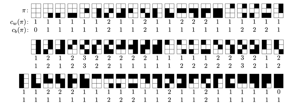
To illustrate the cluster statistics in a small instance, we include the complete enumeration of the \(2^6=64\) binary colorings of \(G_{3,2}\). For each coloring \(\pi\), Figure 1 records the pair \((c_w(\pi),c_b(\pi))\), in a format analogous to [2].
The paper organization is as follows: §2 introduces the bivariate cluster enumerators and the diagonal specialization used to recover the total cluster count. §3 develops the frontier-state transition framework, proves that the full frontier partition is noncrossing, enumerates the principal ambient state spaces, and introduces the block-adjacency graph and the resulting bipartite structural bounds. §4 combines the structural height-four bound with an independently generated labeled transition system to determine the \(27\)-state automaton and derive the exact formulas for \(S_{4,n}\). Finally, §5 first discusses the limitations of the method, the principal open problems, and possible extensions, and then summarizes the conclusions. Appendix A records representative transfer data, the complete terminal vector, and the reproducibility checks; the full matrix \(T_4(p,q)\) is provided in machine-readable form in Supplementary File S2.
For fixed \(m\geq 1\) and \(n\geq 0\), define the bivariate cluster enumerator \(\displaystyle F_{m,n}(p,q) := \sum\limits_{\pi\in\Omega_{m,n}} p^{c_w(\pi)}q^{c_b(\pi)}.\) Mansour’s generating function [2] is then \(\displaystyle F_m(x,p,q) := \sum\limits_{n\geq 0}F_{m,n}(p,q)x^n.\) Because \(\Omega_{m,0}=\{\varnothing\}\) and \(c_w(\varnothing)=c_b(\varnothing)=0\), one has \(F_{m,0}(p,q)=1.\) Introducing a single marking variable \(z\) and specializing \(p=q=z\), one obtains \(\displaystyle F_m(x,z,z) = \sum\limits_{n\geq 0} \left( \sum\limits_{\pi\in\Omega_{m,n}}z^{K(\pi)} \right)x^n.\) Hence, with \(S_{m,n}\) as in (1),
and therefore \(\displaystyle S_{m,n} = [x^n] \left. \frac{d}{dz} F_m(x,z,z) \right|_{z=1}.\) In particular, \(S_{m,0}=0\). The transfer procedure scans a coloring column by column while retaining the connectivity of the clusters that meet the most recently processed column, called the frontier. This is the transfer-matrix/automaton viewpoint of [2].
Fix \(m\geq 1\). We number the rows \(1,\ldots,m\) from top to bottom and the columns from left to right. A column word \(v=(v_1,\ldots,v_m)\in\{0,1\}^m\) is therefore read from top to bottom.
For \(k\geq 0\), a colored prefix of width \(k\) is a coloring \(P\in\Omega_{m,k}.\) If \(k\geq 1\), its frontier is its rightmost column. The unique element of \(\Omega_{m,0}\) is the empty prefix \(\varnothing\), whose state is denoted by \(\langle\varepsilon\rangle\).
If \(P\in\Omega_{m,k}\) and \(v\in\{0,1\}^m\), we write \(P\star v\in\Omega_{m,k+1}\) for the colored prefix obtained by appending \(v\) to the right of \(P\). More generally, if \(w=v^{(1)}\cdots v^{(\ell)}\) is a word of columns, read from left to right, then \(P\star w\) denotes the successive extension of \(P\) by those columns.
Let \(P\in\Omega_{m,k}\) with \(k\geq 1\). A cluster of \(P\) is active if it meets the frontier and is closed otherwise. Let \(C_w(P),C_b(P)\) denote the numbers of closed white and black clusters, and let \(a_w(P),a_b(P)\) denote the corresponding numbers of active clusters. Thus
For the empty prefix, all four quantities are defined to be zero. We associate with every colored prefix the closed-cluster weight
Definition 1 (Frontier state). For a nonempty colored prefix \(P\), its frontier state consists of:
In particular, \(i\sim_P j\) implies \(u_i=u_j\). We denote this frontier state by \(s(P)\). The blocks of \(\sim_P\) are in bijection with the active clusters of \(P\). For the empty prefix, we set \(s(\varnothing):=\langle\varepsilon\rangle.\)
Remark 1 (Canonical encoding). A nonempty frontier state is encoded as \(\langle u,\kappa\rangle,\) where \(u\in\{0,1\}^m\) is the frontier color word and \(\kappa=(\kappa_1,\ldots,\kappa_m)\in\{0,1,2,\ldots\}^m\) satisfies \(\kappa_i=\kappa_j\) if and only if \(i\sim_P j\). The canonical labels are assigned by scanning rows \(1,\ldots,m\) from top to bottom: the first block encountered receives label \(0\), and each subsequently encountered new block receives the next unused integer. This procedure gives a unique encoding of every nonempty frontier state.
For a state \(s\), we write \(a_w(s)\) and \(a_b(s)\) for the numbers of white and black blocks, respectively, and set \(a_w(\langle\varepsilon\rangle)=a_b(\langle\varepsilon\rangle)=0.\) Since the blocks of \(s(P)\) are in bijection with the active clusters of \(P\), one has
for every colored prefix \(P\), including the empty prefix.
Definition 2 (Abstract and reachable state spaces). An abstract nonempty frontier state of height \(m\) is a canonically encoded pair \(s=\langle u,\kappa\rangle\) such that:
Let \(\mathcal U_m\) denote the set of all such abstract nonempty states. For \(s=\langle u,\kappa\rangle\in\mathcal U_m\), define \(\Pi(s)\) as the partition of \([m]\) whose blocks are the equal-label classes of \(\kappa\). The induced block coloring is \(\chi_s(B):=u_i \;\; (i\in B).\) This is well defined by condition \(2\). For \(\xi\in\{0,1\}\), let \(\Pi_\xi(s)\) be the restriction of \(\Pi(s)\) to the positions belonging to blocks of color \(\xi\). The reachable state space is \(\mathcal S_m := \{\langle\varepsilon\rangle\} \cup \bigl\{ s(P): k\geq1,\; P\in\Omega_{m,k} \bigr\}.\) Thus \(\mathcal S_m\setminus\{\langle\varepsilon\rangle\} \subseteq\mathcal U_m.\)
The frontier state is not merely a convenient encoding: it records exactly the connectivity data that can interact with columns appended to the right.
Definition 3 (One-column transition). Let \(s=\langle u,\kappa\rangle\) be a nonempty frontier state of height \(m\), and let \(v\in\{0,1\}^m\). Form an auxiliary graph with old-frontier vertices \(1^{-},\ldots,m^{-}\) and new-frontier vertices \(1^{+},\ldots,m^{+}\) as follows:
The connectedness relation induced on \(1^{+},\ldots,m^{+}\), together with the color word \(v\), defines a unique canonically encoded successor state, denoted by \(\delta(s,v)\).
For a block \(B\) of \(s\), let its color be the common value \(u_i\) for \(i\in B\). Define \(b_w(s,v)\) and \(b_b(s,v)\) as the numbers of white and black blocks \(B\), respectively, for which no \(i\in B\) satisfies \(u_i=v_i\).
For \(v\in\{0,1\}^m\), let \(\kappa(v)\) be the canonical block-label word whose blocks are the maximal monochromatic vertical runs of \(v\). For the empty state, define
and set \(b_w(\langle\varepsilon\rangle,v) = b_b(\langle\varepsilon\rangle,v) = 0.\)
For a word \(w=v^{(1)}\cdots v^{(\ell)}\), extend \(\delta\) recursively by \(\delta(s,\varepsilon)=s\) and \(\delta(s,wv)=\delta(\delta(s,w),v).\)
Proposition 1 (State sufficiency and closed-cluster invariant). Let \(P\in\Omega_{m,k}\) with \(k\geq 0\), let \(s(P)\) be its frontier state, and let \(v\in\{0,1\}^m\). Then
Consequently,
Moreover, for every colored prefix \(P\),
Proof. For a nonempty prefix, the active clusters are in bijection with the blocks of its frontier state. The active cluster represented by a block \(B\) becomes closed after appending \(v\) if and only if none of its frontier cells has a same-colored horizontal neighbor in the new column. Hence the numbers of newly closed white and black clusters are exactly \(b_w(s(P),v)\) and \(b_b(s(P),v)\). Existing closed clusters cannot interact with future columns and remain closed. Every cluster created by cells of the new column meets the new frontier and is therefore active, while a merger of surviving active clusters changes neither \(C_w\) nor \(C_b\). This proves (7) and (8).
The auxiliary graph in Definition 3 records precisely the previous active connectivity, the same-colored horizontal adjacencies to \(v\), and the same-colored vertical adjacencies inside \(v\). Its connected components on the new frontier therefore give \(s(P\star v)\), proving (6) for every nonempty prefix.
If \(P=\varnothing\), Eq. (5) gives \(s(\varnothing\star v)=\delta(\langle\varepsilon\rangle,v).\) Moreover, every cluster of the first column meets the frontier, so \(C_w(\varnothing\star v)=C_b(\varnothing\star v)=0.\) Since \(C_w(\varnothing)=C_b(\varnothing)=0\) and \(b_w(\langle\varepsilon\rangle,v) = b_b(\langle\varepsilon\rangle,v)=0,\) the two closed-cluster update identities also hold for the empty prefix.
Eq. (9) follows immediately from the two closed-cluster updates and the definition of \(W(P)\). Finally, every cluster of \(P\) is either closed or active. Therefore, combining (3) with (4) gives (10). The same identity holds for the empty prefix because all four cluster counts vanish. \(\square\)
Corollary 1 (Weighted scan identity). Let \(\pi\in\Omega_{m,n}\) have column word \(w=v^{(1)}\cdots v^{(n)},\) and define \(s_0=\langle\varepsilon\rangle\) and \(s_j=\delta(s_{j-1},v^{(j)})\) for \(1\leq j\leq n\). Then
For \(n=0\), the product is empty and the terminal factor at \(\langle\varepsilon\rangle\) equals \(1\).
Proof. Iterate (9) from the empty prefix and then apply (10). \(\square\)
Corollary 2 (Compatibility with Mansour’s equivalence). Let \(P_1\) and \(P_2\) be colored prefixes with \(s(P_1)=s(P_2).\) Then, for every finite column word \(w\),
which is independent of \(w\). In particular, \(P_1\) and \(P_2\) are equivalent in the sense of Mansour’s continuation relation.
Proof. Starting from the same frontier state and reading the same continuation word produces the same sequence of successor states, the same sequence of closure counts, and the same terminal active-block counts. The only possible difference is therefore the pair of closed-cluster counts already accumulated in \(P_1\) and \(P_2\), which gives (11). \(\square\)
Proposition 1 shows that frontier states contain all information relevant for future extensions of a prefix. We now establish a planar restriction on the complete connectivity partition of the frontier.
Connectivity partitions arise naturally from the Fortuin–Kasteleyn random-cluster representation [3]. In planar strip transfer matrices, the relevant boundary connectivities are noncrossing, replacing unrestricted Bell-type state spaces by Catalan-type spaces; see the Potts-model framework in [4]. In a percolation setting, Scullard and Jacobsen similarly represent transfer states by planar connectivity partitions of boundary terminals; the Catalan number gives the dimension of the transfer space, and the construction is applied to both bond and site percolation [5]. Recent algebraic treatments of related noncrossing connectivity spaces appear in [6,7]. Theorem 1 specializes this established planar principle to the complete bicromatic active-cluster states used in the present enumeration problem.
Definition 4 (Noncrossing partition). Let \(I\) be a finite linearly ordered set. A partition \(\mathcal P\) of \(I\) is noncrossing if there do not exist elements \(a<b<c<d\) of \(I\) and two distinct blocks \(B_1,B_2\in\mathcal P\) such that \(a,c\in B_1\) and \(b,d\in B_2.\)
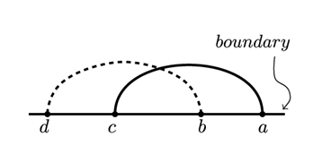
Lemma 1 (Alternating boundary pairs). Let \(D\) be a closed topological disk, and let \(x_a,x_b,x_c,x_d\in\partial D\) be distinct boundary points occurring in this cyclic order. There do not exist two disjoint simple arcs \(A_1,A_2\subseteq D\) such that:
Proof. The arc \(A_1\) is a crosscut of the disk. By the crosscut theorem, which is a standard consequence of the Jordan curve theorem, the set \(D\setminus A_1\) has exactly two connected components. The two open boundary arcs of \(\partial D\setminus\{x_a,x_c\}\) lie on different sides of \(A_1\). Since the four boundary points occur in alternating cyclic order, \(x_b\) and \(x_d\) belong to different boundary arcs between \(x_a\) and \(x_c\). Consequently, every connected subset of \(D\) joining \(x_b\) to \(x_d\) must meet \(A_1\). In particular, \(A_2\cap A_1\neq\varnothing\), contradicting the assumed disjointness. \(\square\)
Definition 5 (Full frontier partition). Let \(P\in\Omega_{m,k}\) be a nonempty colored prefix. Its full frontier partition is
where \(\sim_P\) is the frontier equivalence relation of Definition 1. Thus two rows belong to the same block of \(\Pi(P)\) if and only if their frontier cells belong to the same active cluster. In the notation of Definition 2,
For \(\xi\in\{0,1\}\), let \(\Pi_\xi(P)\) denote the restriction of \(\Pi(P)\) to the rows whose frontier color is \(\xi\). Equivalently, \(\Pi_\xi(P)=\Pi_\xi(s(P)).\)
Theorem 1 (Noncrossing full frontier partition). For every nonempty colored prefix \(P\), the full frontier partition \(\Pi(P)\) is noncrossing.
Proof. Suppose, to the contrary, that \(\Pi(P)\) is crossing. Then there exist rows \(a<b<c<d\) and two distinct blocks \(B_1,B_2\in\Pi(P)\) such that \(a,c\in B_1\) and \(b,d\in B_2.\)
Let \(C_1\) and \(C_2\) be the active clusters represented by \(B_1\) and \(B_2\), respectively. Since the frontier cells in rows \(a\) and \(c\) belong to \(C_1\), there is a simple path \(Q_1\subseteq C_1\) joining them. Likewise, there is a simple path \(Q_2\subseteq C_2\) joining the frontier cells in rows \(b\) and \(d\). Because \(C_1\neq C_2\), the paths \(Q_1\) and \(Q_2\) are vertex-disjoint. This remains true whether the two clusters have the same color or different colors.
Embed the grid graph of the prefix in the interior of a closed rectangle \(D\), placing the rightmost grid column strictly to the left of the right side of \(D\). Thus there is an open vertical strip between the frontier and the right boundary of \(D\) that is disjoint from the embedded grid.
For each \(r\in\{a,b,c,d\}\), join the frontier vertex in row \(r\) to a point \(x_r\) on the right boundary of \(D\) by an arc contained in this strip. These four extensions can be chosen pairwise disjoint. The points \(x_a,x_b,x_c,x_d\) occur on \(\partial D\) in this cyclic order.
The embedded path \(Q_1\), together with the extensions at its endpoints, forms a simple arc \(A_1\) joining \(x_a\) to \(x_c\), whose interior lies in the interior of \(D\). Similarly, \(Q_2\) determines a simple arc \(A_2\) joining \(x_b\) to \(x_d\). Since \(Q_1\) and \(Q_2\) lie in distinct clusters and the four extensions are pairwise disjoint, the arcs \(A_1\) and \(A_2\) are disjoint. This contradicts Lemma 1. Therefore \(\Pi(P)\) is noncrossing. \(\square\)
Corollary 3 (Colorwise noncrossing). For every nonempty colored prefix \(P\) and each color \(\xi\in\{0,1\},\) the restricted partition \(\Pi_\xi(P)\) is noncrossing.
Proof. A restriction of a noncrossing partition to a subset of its underlying ordered set is again noncrossing. The result therefore follows from Theorem 1. \(\square\)
Remark 2 (Finiteness versus noncrossing). The finiteness of the state space at fixed height does not depend on Theorem 1: a state is determined by a binary word in \(\{0,1\}^m\) and an equivalence relation on \([m]\), so only finitely many states exist. The role of Theorem 1 is sharper: it excludes crossing equivalence relations and replaces an unrestricted Bell-type ambient family by a noncrossing, Catalan-type family.
Figure 2 illustrates the alternating-boundary configuration excluded by Lemma 1 and used in the proof of Theorem 1.
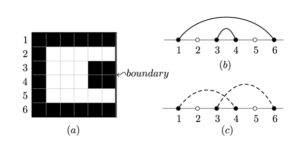
A convenient visualization of Corollary 3 is obtained by representing the frontier rows \(1,\ldots,m\) on a horizontal line and drawing arcs between positions that belong to the same active cluster of one selected color.
Figure 3 illustrates the one-color restriction for a prefix of height \(m=6\). In panel (a), the frontier intersects two black active clusters, one meeting the frontier in rows \(\{1,6\}\) and the other in rows \(\{3,4\}\). Panel (b) shows the corresponding noncrossing arc diagram. Panel (c) displays a crossing restriction, which cannot arise by Corollary 3.
The noncrossing results define several natural ambient classes between arbitrary abstract states and reachable states.
Definition 6 (Colorwise and full noncrossing spaces). Let \(\mathcal C_m := \bigl\{ s\in\mathcal U_m: \Pi_0(s)\text{ and }\Pi_1(s)\text{ are noncrossing} \bigr\},\) and let \(\mathcal N_m := \bigl\{ s\in\mathcal U_m: \Pi(s)\text{ is noncrossing} \bigr\}.\)
Proposition 2 (Exact ambient-state counts). For \(r\geq0\), let \(\displaystyle C_r := \frac{1}{r+1}\binom{2r}{r}\) be the \(r\)-th Catalan number; in particular, \(C_0=1\). For \(1\leq k\leq m\), let \(\mathrm S(m,k)\) denote the Stirling number of the second kind, and let \(\displaystyle \mathrm{Nar}(m,k) := \frac{1}{m} \binom{m}{k} \binom{m}{k-1}\) be the Narayana number. Then
Moreover, \(\mathcal N_m \subseteq \mathcal C_m \subseteq \mathcal U_m.\)
Proof. An element of \(\mathcal U_m\) is determined by a partition of \([m]\) into \(k\) blocks and an arbitrary binary color assigned to each block. There are \(\mathrm S(m,k)\) choices for the partition and \(2^k\) block colorings, proving (12).
To construct an element of \(\mathcal C_m\), choose the \(i\) white positions, a noncrossing partition of those positions, and a noncrossing partition of the remaining black positions. This gives \(\binom{m}{i}C_iC_{m-i}\) states for each \(i\), proving (12).
Finally, a noncrossing partition of \([m]\) with \(k\) blocks can be chosen in \(\mathrm{Nar}(m,k)\) ways, and its blocks can be colored independently in \(2^k\) ways. This proves (12).
A restriction of a noncrossing partition is noncrossing, so \(\mathcal N_m\subseteq\mathcal C_m.\) The second inclusion is immediate from the definitions. \(\square\)
Corollary 4 (Full-frontier noncrossing bound). For every \(m\geq1\), \(\mathcal S_m\setminus\{\langle\varepsilon\rangle\} \subseteq \mathcal N_m,\) and consequently \(|\mathcal S_m|-1 \leq |\mathcal N_m| = R_m \leq 8^m.\) In particular, \(|\mathcal S_4|-1 \leq R_4 = 90.\)
Proof. The inclusion follows from Theorem 1. The cardinality of \(\mathcal N_m\) is given by Proposition 2. Moreover, \(R_m \leq 2^m \sum\limits_{k=1}^{m}\mathrm{Nar}(m,k) = 2^m C_m \leq 8^m.\) For \(m=4\), the Narayana numbers are \(1,6,6,1\), and hence \(R_4 = 2+6\cdot2^2+6\cdot2^3+2^4 = 90.\) \(\square\)
Remark 3 (Meaning of the three ambient counts). The quantities in Proposition 2 count different classes:
Thus the former product-Catalan upper bound is the exact cardinality of \(\mathcal C_m\), not the number of reachable or simultaneously realizable states.
Remark 4 (Relation with colored set partitions). The colorwise class \(\mathcal C_m\) is related to enumerative models of colored set partitions in which crossings are restricted within each color; see [8]. The two settings are not identical: in the present model colors are assigned to blocks rather than to individual arcs, while the subclasses \(\mathcal N_m\) and \(\mathcal B_m\) impose additional compatibility conditions arising from the planar grid and from adjacency of consecutive frontier positions.
Proposition 3 (Schröder interpretation and growth). Set \(R_0:=1\) and define \(\mathcal R(x):=\sum\limits_{m\geq0}R_mx^m.\) Then \(R_m\) is the \(m\)-th large Schröder number and
Consequently,
and
In particular,
Proof. The identity \(R_m=\sum\limits_{k=1}^{m}\mathrm{Nar}(m,k)2^k\) is the standard Narayana-polynomial representation of the large Schröder numbers; see, for example, [9]. Their first-return decomposition gives (13), from which (14) and (15) follow. The dominant singularity of \(\mathcal R(x)\) is \(3-2\sqrt2,\) and the square-root singularity in (14) gives (16). \(\square\)
The bound \(R_m\) still allows arbitrary binary colorings of the blocks of a noncrossing partition. Frontier adjacency imposes an additional restriction.
Definition 7 (Block-adjacency graph). Let \(\Pi\) be a partition of \([m]\). For \(i\in[m]\), denote by \(B_\Pi(i)\) the block of \(\Pi\) containing \(i\). The block-adjacency graph \(Q(\Pi)\) is the simple graph whose vertex set is the set of blocks of \(\Pi\), with an edge between two distinct blocks \(B\) and \(B’\) if there exists \(i\in[m-1]\) such that \(B_\Pi(i)=B\) and \(B_\Pi(i+1)=B’.\)
Lemma 2 (Connectivity of the block-adjacency graph). For every partition \(\Pi\) of \([m]\), the graph \(Q(\Pi)\) is connected.
Proof. Consider the sequence of blocks \(B_\Pi(1),B_\Pi(2),\ldots,B_\Pi(m).\) Delete each term that is equal to its immediate predecessor. The resulting sequence still visits every block of \(\Pi\), and every pair of consecutive terms consists of distinct blocks containing two consecutive positions of \([m]\). Hence consecutive terms are adjacent in \(Q(\Pi)\). The reduced sequence therefore contains a walk from \(B_\Pi(1)\) to every block of \(\Pi\), and \(Q(\Pi)\) is connected. \(\square\)
Proposition 4 (Bipartite compatibility). Let \(P\) be a nonempty colored prefix with frontier color word \(u=(u_1,\ldots,u_m)\) and full frontier partition \(\Pi(P)\). Assign to each block \(B\in\Pi(P)\) its common frontier color
Then \(\chi_P\) is a proper two-coloring of \(Q(\Pi(P))\). Consequently, \(Q(\Pi(P))\) is bipartite.
Proof. The map \(\chi_P\) is well defined because all positions in a block belong to the same monochromatic active cluster. Let \(B\) and \(B’\) be adjacent vertices of \(Q(\Pi(P))\). Then there exists \(i\in[m-1]\) such that \(i\in B\) and \(i+1\in B’.\) If \(\chi_P(B)=\chi_P(B’)\), the two frontier cells in rows \(i\) and \(i+1\) are vertically adjacent and have the same color. They therefore belong to the same active cluster, which would imply \(B=B’\), a contradiction. Hence \(\chi_P(B)\neq\chi_P(B’),\) so \(\chi_P\) is proper. \(\square\)
Definition 8 (Bipartite noncrossing states). Let \(\mathfrak B_m\) be the set of noncrossing partitions \(\Pi\) of \([m]\) for which \(Q(\Pi)\) is bipartite, and define \(b_m:=|\mathfrak B_m|.\) Define \(\mathcal B_m := \bigl\{ s\in\mathcal N_m: \chi_s\text{ is a proper two-coloring of }Q(\Pi(s)) \bigr\}.\)
Corollary 5 (Bipartite structural bound). For every \(m\geq1\), \(\mathcal S_m\setminus\{\langle\varepsilon\rangle\} \subseteq \mathcal B_m \subseteq \mathcal N_m \subseteq \mathcal C_m \subseteq \mathcal U_m,\) and \(|\mathcal B_m|=2b_m.\) Consequently,
Proof. The inclusion follows from Theorem 1 and Proposition 4. By Lemma 2, every \(Q(\Pi)\) is connected. Hence, whenever it is bipartite, it has exactly two proper two-colorings, which differ by global color complementation. Therefore \(|\mathcal B_m|=2b_m.\) The remaining inclusions follow from the definitions of \(\mathcal B_m,\mathcal N_m,\mathcal C_m\) and \(\mathcal U_m\). Their cardinalities are given by Proposition 2, yielding the full chain (17). \(\square\)
Corollary 6 (The structural bound at height \(4\)). For \(m=4\), \(b_4=13, \;\; |\mathcal B_4|=26,\) and therefore \(|\mathcal S_4|\leq27.\)
Proof. There are \(C_4=14\) noncrossing partitions of \([4]\). For any partition of \([4]\), the graph \(Q(\Pi)\) has at most three edges, one for each pair of consecutive positions. If \(Q(\Pi)\) is nonbipartite, then, being connected, it must contain an odd cycle. Since it has at most three edges, this odd cycle must be a triangle. Thus the three consecutive pairs \((1,2),(2,3),(3,4)\) must induce three distinct edges among three blocks. This occurs if and only if \(B_\Pi(1)=B_\Pi(4)\) and \(B_\Pi(1),B_\Pi(2),B_\Pi(3)\) are pairwise distinct. Hence the unique noncrossing partition with nonbipartite block-adjacency graph is \(\bigl\{\{1,4\},\{2\},\{3\}\bigr\},\) whose block-adjacency graph is a triangle. Therefore \(13\) of the \(14\) noncrossing partitions belong to \(\mathfrak B_4\), so \(b_4=13\). Corollary 5 gives \(|\mathcal S_4|-1\leq2b_4=26.\) \(\square\)
The exact reachable-state counts, the bipartite structural bound \(2b_m\), and the full-frontier bound \(R_m\) are shown in Table 1. All counts exclude the initial state.
| \(m\) | \(|\mathcal S_m|-1\) | \(2b_m\) | \(R_m\) |
|---|---|---|---|
| 1 | 2 | 2 | 2 |
| 2 | 4 | 4 | 6 |
| 3 | 10 | 10 | 22 |
| 4 | 26 | 26 | 90 |
| 5 | 72 | 72 | 394 |
| 6 | 206 | 206 | 1806 |
| 7 | 608 | 608 | 8558 |
| 8 | 1834 | 1834 | 41586 |
The exact enumeration gives \((b_1,\ldots,b_8) = (1,2,5,13,36,103,304,917).\) For every \(1\leq m\leq8\), the reachable-state count attains the bipartite structural bound: \(|\mathcal S_m|-1=2b_m.\) This equality is verified by Supplementary File S1. Its structurally independent modules enumerate the noncrossing partitions and their block-adjacency graphs, regenerate the reachable-state sets by breadth-first search, and compare the resulting values of \(2b_m\) and \(|\mathcal S_m|-1\) for every \(1\leq m\leq8\). For \(m=4\), equality follows without relying on the enumeration of all transitions: Corollary 6 gives the upper bound \(26\), while Table 2 provides \(26\) distinct nonempty reachable states.
| State | Witness | State | Witness | State | Witness | State | Witness | State | Witness |
|---|---|---|---|---|---|---|---|---|---|
| \(s_0\) | \(\varepsilon\) | \(s_6\) | \(0101\) | \(s_{12}\) | \(1011\) | \(s_{18}\) | \(0000\,0100\) | \(s_{24}\) | \(1110\,1010\) |
| \(s_1\) | \(0000\) | \(s_7\) | \(0110\) | \(s_{13}\) | \(1100\) | \(s_{19}\) | \(0000\,0101\) | \(s_{25}\) | \(1110\,1011\) |
| \(s_2\) | \(0001\) | \(s_8\) | \(0111\) | \(s_{14}\) | \(1101\) | \(s_{20}\) | \(0000\,0110\) | \(s_{26}\) | \(1111\,1001\) |
| \(s_3\) | \(0010\) | \(s_9\) | \(1000\) | \(s_{15}\) | \(1110\) | \(s_{21}\) | \(0000\,1010\) | ||
| \(s_4\) | \(0011\) | \(s_{10}\) | \(1001\) | \(s_{16}\) | \(1111\) | \(s_{22}\) | \(0111\,0101\) | ||
| \(s_5\) | \(0100\) | \(s_{11}\) | \(1010\) | \(s_{17}\) | \(0000\,0010\) | \(s_{23}\) | \(0111\,1101\) |
Conjecture 1 (Bipartite characterization of reachability). For every \(m\geq1\), \(\mathcal S_m\setminus\{\langle\varepsilon\rangle\} = \mathcal B_m.\) Equivalently, a canonically encoded nonempty abstract state is reachable if and only if its full frontier partition is noncrossing and the block coloring induced by its frontier color word is a proper two-coloring of its block-adjacency graph.
Problem 1 (Constructive realization). Construct, for every \(\Pi\in\mathfrak B_m\) and every proper two-coloring of \(Q(\Pi)\), a colored prefix whose frontier state realizes the corresponding element of \(\mathcal B_m\).
In this section we determine the reachable frontier-state automaton for height \(m=4\), derive the associated transfer matrix, and obtain an explicit closed formula for \(\displaystyle S_{4,n} = \sum\limits_{\pi\in\Omega_{4,n}}K(\pi).\) Corollary 6 gives the sharp structural upper bound \(|\mathcal S_4|-1\leq26.\) The \(26\) nonempty states listed below have explicit reachability witnesses. Hence the upper bound is attained, and the automaton has exactly \(27\) states after adjoining the initial state.
For \(m=4\), the frontier-state automaton is constructed by a breadth-first search starting from the initial state \(\langle\varepsilon\rangle\) and using the transition operator of Definition 3. For every discovered state \(s\) and every column \(v\in\{0,1\}^{4}\), the algorithm computes the successor \(\delta(s,v)\) and the closure counts \(b_w(s,v)\) and \(b_b(s,v)\).
For a nonempty state, the auxiliary graph of Definition 3 has eight frontier vertices and is implemented by a union–find structure. The initial transition from \(\langle\varepsilon\rangle\) is handled by the separate width-zero clause of that definition. At fixed height \(m\), a nonempty state is determined by a binary word in \(\{0,1\}^m\) and an equivalence relation on \([m]\) compatible with that word. Hence only finitely many canonical states exist, and the breadth-first search eventually stabilizes.
The breadth-first computation uses exact integer data and the canonical encoding of Remark 1. Supplementary File S1 is a deterministic exact-arithmetic verification package. Its frontier-state module regenerates the reachable-state sets, minimal witnesses, closure counts, and labeled transitions directly from Definition 3, without reading Supplementary File S2. Supplementary File S2 is the independent machine-readable transition certificate for \(m=4\), consisting of the \(27\cdot16=432\) records
When executed against Supplementary File S2, the package compares the regenerated data with the certificate entry by entry and writes the exact results to verification_report.json. This report is generated at run time and is not a separate supplementary file.
Because the search processes states in nondecreasing distance from \(\langle\varepsilon\rangle\), the first word recorded for each state has minimum possible length. Thus the witnesses in Table 2 are shortest column words reaching their corresponding states.
Example 1 (A complete transition). Consider the state \(s=\langle(0101),(0123)\rangle\) and append the column \(v=(0111).\)
The old frontier has color pattern \(0101\). Its four active blocks are all distinct: the white cells in rows \(1\) and \(3\) belong to two different white clusters, and the black cells in rows \(2\) and \(4\) belong to two different black clusters. After appending \(v=(0111)\), the horizontal adjacencies are as follows: row \(1\) connects old \(0\) to new \(0\), row \(2\) connects old \(1\) to new \(1\), row \(3\) does not connect because \(0\neq1\), and row \(4\) connects old \(1\) to new \(1\).
Inside the new column, the black cells in rows \(2,3,4\) are vertically adjacent, hence they form a single active black block. Therefore the two old black clusters meeting rows \(2\) and \(4\) merge into one active black cluster in the new frontier. The old white cluster in row \(1\) remains active, while the old white cluster in row \(3\) has no horizontal connection to the new column and therefore closes.
Thus the new frontier consists of one active white block (meeting row \(1\)) and one active black block (meeting rows \(2,3,4\)).
After canonical relabeling, the white block receives label \(0\) and the black block receives label \(1\). Therefore \(\delta(s,v) = \langle(0111),(0111)\rangle.\) Moreover, \(b_w(s,v)=1, \;\; b_b(s,v)=0.\) Hence the corresponding contribution to \(T_4(p,q)\) is \(p.\)
Proposition 5 (Labeled transition-system certificate). Let \(\mathcal A=\{s_0,\ldots,s_{26}\}\) be the ordered state set of Table 3. Supplementary File S2 contains exactly one transition record for every pair \((s_i,v)\in\mathcal A\times\{0,1\}^{4}.\) Every recorded successor belongs to \(\mathcal A\). Consequently, the certificate defines a complete closed deterministic transition system on \(\mathcal A\) with \(27\cdot16=432\) labeled transitions.
| Index | State | Index | State | Index | State |
|---|---|---|---|---|---|
| 0 | \(\langle\varepsilon\rangle\) | 1 | \(\langle(0000),(0000)\rangle\) | 2 | \(\langle(0001),(0001)\rangle\) |
| 3 | \(\langle(0010),(0012)\rangle\) | 4 | \(\langle(0011),(0011)\rangle\) | 5 | \(\langle(0100),(0122)\rangle\) |
| 6 | \(\langle(0101),(0123)\rangle\) | 7 | \(\langle(0110),(0112)\rangle\) | 8 | \(\langle(0111),(0111)\rangle\) |
| 9 | \(\langle(1000),(0111)\rangle\) | 10 | \(\langle(1001),(0112)\rangle\) | 11 | \(\langle(1010),(0123)\rangle\) |
| 12 | \(\langle(1011),(0122)\rangle\) | 13 | \(\langle(1100),(0011)\rangle\) | 14 | \(\langle(1101),(0012)\rangle\) |
| 15 | \(\langle(1110),(0001)\rangle\) | 16 | \(\langle(1111),(0000)\rangle\) | 17 | \(\langle(0010),(0010)\rangle\) |
| 18 | \(\langle(0100),(0100)\rangle\) | 19 | \(\langle(0101),(0102)\rangle\) | 20 | \(\langle(0110),(0110)\rangle\) |
| 21 | \(\langle(1010),(0121)\rangle\) | 22 | \(\langle(0101),(0121)\rangle\) | 23 | \(\langle(1101),(0010)\rangle\) |
| 24 | \(\langle(1010),(0102)\rangle\) | 25 | \(\langle(1011),(0100)\rangle\) | 26 | \(\langle(1001),(0110)\rangle\) |
Proof. Supplementary File S2 contains the records \((s_i,v,\delta(s_i,v),b_w(s_i,v),b_b(s_i,v))\) for all \((s_i,v)\in\mathcal A\times\{0,1\}^{4}.\) The frontier-state module of Supplementary File S1 independently regenerates these records directly from Definition 3, without using the contents of Supplementary File S2. The certificate-verification module then compares the regenerated records with Supplementary File S2 and checks that there are exactly \(432\) distinct source-label pairs, that every source has exactly \(16\) records, and that every successor has an index in \(\{0,\ldots,26\}\). Hence the labeled transition system stored in Supplementary File S2 is complete and closed on \(\mathcal A\). \(\square\)
Proposition 6 (Reachable state space for \(m=4\)). For height \(m=4\), the set of reachable frontier states is precisely the set \(\mathcal A\) listed in Table 3. In particular, \(\mathcal S_4=\mathcal A \;\;\text{and}\;\; |\mathcal S_4|=27.\)
Proof. Let \(\mathcal A=\{s_0,\ldots,s_{26}\}\) be the collection of states listed in Table 3. For each \(s_i\in\mathcal A\), Table 2 provides a column word \(w_i\) satisfying \(\delta(\langle\varepsilon\rangle,w_i)=s_i.\) Hence \(\mathcal A\subseteq\mathcal S_4.\) In particular, \(|\mathcal S_4|\geq27.\) On the other hand, Corollary 6 gives \(|\mathcal S_4|\leq27.\) Therefore \(|\mathcal S_4|=27.\) Since \(\mathcal A\) consists of \(27\) distinct reachable states, it follows that \(\mathcal S_4=\mathcal A.\) \(\square\)
The equality \(|\mathcal S_4|-1=26=2b_4\) shows that every bipartite noncrossing state of height \(4\) is reachable. Thus the state count is not merely the output of the breadth-first search: it follows from the \(13\) admissible noncrossing partitions, their two complementary proper block colorings, and the explicit reachability witnesses.
The unique noncrossing partition excluded by the bipartite condition is \(\{\{1,4\},\{2\},\{3\}\},\) whose block-adjacency graph is a triangle.
We denote by \(\mathcal A=\{s_0,\ldots,s_{26}\}\) the set of states listed in Table 3, where the index of each row determines the ordering used throughout the paper. This ordering is used in the definition of the transfer matrix \(T_4(p,q)\) in the next subsection.
Let \(T_4(p,q)\) be the bivariate transfer matrix associated with the \(27\) reachable frontier states obtained in Proposition 6. For \(s,t\in\mathcal S_4\), the corresponding transfer-matrix entry is defined by
Thus every input column contributes the closed-cluster weight prescribed by (9). Let \(e_{\varepsilon}^{\mathsf T}\) be the row vector whose coordinate at \(\langle\varepsilon\rangle\) is \(1\) and whose remaining coordinates are \(0\). Define the terminal column vector \(\mathbf w_4(p,q)\) by
In particular, \(\bigl(\mathbf w_4(p,q)\bigr)_{\langle\varepsilon\rangle}=1.\) The weighted scan identity gives \(F_4(x,p,q) = e_{\varepsilon}^{\mathsf T} (I-xT_4(p,q))^{-1} \mathbf w_4(p,q),\)
Lemma 3 (Correctness of the terminal vector). Let \(P\) be a colored prefix with terminal state \(t=s(P)\). Then
In particular, every monochromatic cluster contributes exactly once: either through a transition weight when it becomes closed, or through the terminal coordinate if it remains active in the final frontier.
Proof. By (19), \(\bigl(\mathbf w_4(p,q)\bigr)_t = p^{a_w(t)}q^{a_b(t)}.\) Eq. (20) is therefore exactly the terminal decomposition (10). \(\square\)
Remark 5. For \(m=2\), the construction recovers exactly the transfer matrix and generating function obtained by Mansour [2].
Proposition 7 (Reconstruction from the labeled transition certificate). In the state ordering of Table 3, Supplementary File S2 uniquely determines the matrix \(T_4(p,q)\) and the terminal vector \(\mathbf w_4(p,q)\). More precisely,
and \(\bigl(\mathbf w_4(p,q)\bigr)_{s_i} = p^{a_w(s_i)}q^{a_b(s_i)}.\) The resulting \(27\times27\) polynomial matrix and the terminal-vector exponents are stored explicitly in Supplementary File S2. Appendix A records representative entries, the complete terminal vector, and the reproducibility checks.
Proof. The transition certificate contains exactly one record for every pair \((s_i,v)\in\mathcal A\times\{0,1\}^{4}.\) Grouping the records by their ordered source-target pair \((s_i,s_j)\) and summing their monomial weights gives the displayed matrix entry. The terminal-vector entry is obtained directly from the white and black active-block counts recorded for \(s_i\). This reconstructs all matrix and terminal-vector coordinates without any additional choices. \(\square\)
Lemma 4 (Exact rational form of \(G_4(x)\)). Let \(F_4(x,p,q) = e_{\varepsilon}^{\mathsf T} (I-xT_4(p,q))^{-1} \mathbf w_4(p,q),\) where \(T_4(p,q)\) is defined by (18) and reconstructed from Supplementary File S2, and where \(\mathbf w_4(p,q)\) is defined by (19). Then
Proof. Expanding the resolvent gives \(\displaystyle e_{\varepsilon}^{\mathsf T} (I-xT_4(p,q))^{-1} \mathbf w_4(p,q) = \sum\limits_{n\geq0} x^n e_{\varepsilon}^{\mathsf T} T_4(p,q)^n \mathbf w_4(p,q).\) For each \(n\), the matrix product on the right sums over all words of \(n\) columns. By (18), the weight of a path is the product of its closed-cluster transition weights. Corollary 1 and Lemma 3 show that, after multiplication by the terminal coordinate, the path associated with \(\pi\in\Omega_{4,n}\) contributes exactly \(p^{c_w(\pi)}q^{c_b(\pi)}.\) Therefore the series is \(F_4(x,p,q)\).
Specializing \(p=q=z\), differentiating with respect to \(z\), and evaluating at \(z=1\) gives \(G_4(x)\) by (2). Exact symbolic simplification yields (21). The analytic module of Supplementary File S1 reproduces this rational function with exact symbolic arithmetic and verifies the coprimality of its numerator and denominator, the minimal recurrence, the partial-fraction decomposition, the closed formula, the quadratic transient recurrence, and the asymptotic densities. The transfer and recurrence identities are checked through \(n=80\), and the closed formula is checked through \(n=24\). \(\square\)
Remark 6 (Independent exact coefficient checks). As a check independent of the frontier-state construction, we exhaustively enumerated all \(2^{4n}\) binary colorings of \(G_{4,n}\) for \(0\leq n\leq5\), computing monochromatic connected components directly in the grid. This gives
These values agree with the transfer-matrix computation and with the series expansion of \(G_4(x)\). Exact transfer iteration further gives
These values again agree with the rational generating function. The direct enumeration and transfer checks are executed by Supplementary File S1. The direct-enumeration module computes connected components directly in the grid and does not import or use the frontier-state implementation. The exact values and their pass/fail status are written to the generated file verification_report.json.
Proposition 8 (Reduced denominator). Let \(N_4(x)=2x(20-288x+889x^2-415x^3-215x^4),\) \(D_4(x)= (1-x)(1-16x)^2(1-3x-x^2).\) Then \(\gcd\bigl(N_4(x),D_4(x)\bigr)=1\) in \(\mathbb Q[x]\). Hence (21) is in reduced form.
Proof. Write \(N_4(x)=2xP(x),\) where \(P(x)=20-288x+889x^2-415x^3-215x^4.\) Since \(D_4(0)=1\), the factor \(x\) is not common. Moreover, \(\displaystyle P(1)=-9, \quad P\left(\frac1{16}\right)=\frac{351801}{65536},\) so neither \(1-x\) nor \(1-16x\) divides \(N_4(x)\). Dividing \(P(x)\) by \(1-3x-x^2\) gives remainder \(4-10x\). A common zero of \(P(x)\) and \(1-3x-x^2\) would therefore have to equal \(2/5\), but \(1-\frac65-\frac4{25} = -\frac9{25} \neq0.\) Thus no irreducible factor of \(D_4(x)\) divides \(N_4(x)\). \(\square\)
We now extract coefficients from the rational form of \(G_4(x)\).
Theorem 2 (Closed formula for \(m=4\)). Set \(\displaystyle \lambda_{\pm} := \frac{3\pm\sqrt{13}}{2}, \quad \alpha_{\pm} := \frac{362}{14283} \pm \frac{1390}{185679}\sqrt{13}.\) Then, for every \(n\geq1\),
Proof. By Lemma 4, \(\displaystyle G_4(x) = \frac{N_4(x)}{D_4(x)}.\) Since \(1-3x-x^2=(1-\lambda_+x)(1-\lambda_-x),\) partial fractions give \(\displaystyle G_4(x) = -\frac{215}{128} + \frac{2}{75}\frac{1}{1-x} + \frac{16389197}{22852800}\frac{1}{1-16x} + \frac{39089}{44160}\frac{1}{(1-16x)^2} + \alpha_+\frac{1}{1-\lambda_+x} + \alpha_-\frac{1}{1-\lambda_-x}.\) The constant polynomial term \(-215/128\) contributes only to the coefficient of \(x^0\). Therefore, for \(n\geq1\),
Finally, \(\displaystyle \frac{39089}{44160}(n+1) + \frac{16389197}{22852800} = \frac{39089}{44160}n + \frac{73235509}{45705600},\) which proves (22). \(\square\)
Corollary 7 (Minimal linear recurrence). The sequence \(\{S_{4,n}\}_{n\geq0}\) satisfies
for \(n\geq6\), with initial values \((S_{4,0},\ldots,S_{4,5}) = (0,40,864,17442,337058,6321014).\) Moreover, no homogeneous constant-coefficient recurrence of smaller order is eventually satisfied by \(\{S_{4,n}\}\).
Proof. The denominator in (21) expands as \(D_4(x) = 1-36x+386x^2-1087x^3+480x^4+256x^5.\) Comparing coefficients in \(D_4(x)G_4(x)=N_4(x)\) for \(n\geq6\) gives (23). The initial values follow from Remark 6.
By Proposition 8, \(G_4(x)\) has reduced denominator of degree \(5\). Hence an eventual homogeneous recurrence of order smaller than \(5\) would give a rational representation with a denominator of smaller degree, contradicting reducedness. \(\square\)
Corollary 8 (Quadratic transient). For \(n\geq1\), define
Then
and consequently
Proof. Eq. (25) follows from Theorem 2. Since \(\lambda_+\) and \(\lambda_-\) are the roots of \(t^2-3t-1,\) each sequence \(\lambda_\pm^n\) satisfies (26). \(\square\)
Corollary 9 (Exact expectation and asymptotics). For \(n\geq1\), set \(\displaystyle r_{\pm} := \frac{\lambda_\pm}{16} = \frac{3\pm\sqrt{13}}{32}.\) Then
Proof. Since \(|\Omega_{4,n}|=16^n\), one has \(\mathbb E_{4,n}[K]=S_{4,n}/16^n.\) Dividing (22) by \(16^n\) gives (27). Moreover,
Therefore all three exponentially decaying terms in (27) are \(O(r_+^n)\). \(\square\)
Corollary 10 (Asymptotic cluster density). For a coloring chosen uniformly from \(\Omega_{4,n}\),
By color symmetry, \(\displaystyle \lim_{n\to\infty} \frac{\mathbb E_{4,n}[c_w]}{4n} = \lim_{n\to\infty} \frac{\mathbb E_{4,n}[c_b]}{4n} = \frac{39089}{353280}.\)
Proof. Divide (28) by \(4n\) and let \(n\to\infty\). The second statement follows from the color-complementation bijection on \(\Omega_{4,n}\). \(\square\)
Remark 7 (Fixed-height densities). For fixed \(m\), define \(\displaystyle \rho_m := \lim_{n\to\infty} \frac{\mathbb E_{m,n}[K]}{mn},\) whenever the limit exists. Mansour’s exact formulas for \(m\leq3\) [2], together with Corollary 10, give
The four displayed values decrease, but no monotonicity assertion for all \(m\) is made.
These are all-cluster strip densities with \(m\) fixed and \(n\to\infty\). The corresponding density for one selected color is \(\rho_m/2\), by color symmetry. Richey [1] adopts the one-color percolation convention and explains the resulting factor \(2\) under the uniform measure. The fixed-height limits above must also be distinguished from the two-dimensional limit in which both \(m\) and \(n\) tend to infinity.
Remark 8 (Relation to previous work and scope of the contribution). Mansour [2] established the finite-automaton framework for this cluster-enumeration problem and obtained exact formulas for heights \(m\leq3\). Theorem 2 extends the exact enumeration to height \(4\).
The use of noncrossing connectivity partitions in planar transfer matrices predates the present work, in both Potts-model and percolation applications; see [4,5]. In particular, Scullard and Jacobsen use planar partitions of boundary terminals as transfer states, with Catalan dimension, in computations of generalized critical polynomials for bond and site percolation. Accordingly, Theorem 1 is not presented as a new general principle for planar transfer matrices. Its role is to formulate that established principle rigorously for the complete bicromatic cluster states of the present enumeration problem.
The new structural refinement is the block-adjacency graph \(Q(\Pi)\) and the proper two-coloring condition of Proposition 4. To the best of my knowledge, this criterion and its use to derive the exact \(27\)-state count have not previously appeared in the binary cluster-enumeration setting. The cardinality is proved structurally by Corollary 6 and the reachability witnesses of Table 2. Separately, Proposition 5 identifies Supplementary File S2 as the complete labeled transition certificate, while Supplementary File S1 independently regenerates and compares all \(432\) transition records.
The present work has three principal limitations.
First, the noncrossing and bipartite conditions are proved to be necessary for reachability at every height, but their sufficiency is established only for \(m=4\). Exact computations verify \(\mathcal S_m\setminus\{\langle\varepsilon\rangle\} = \mathcal B_m\) for \(1\leq m\leq8\), but these finite checks do not constitute a proof for arbitrary \(m\). The main structural problem is therefore Conjecture 1. Its constructive form is stated in Problem 1: one must build a colored prefix realizing every properly two-colored noncrossing partition with bipartite block-adjacency graph.
Second, although the frontier-state procedure applies in principle to every fixed height \(m\), the exact transfer-matrix analysis has been carried out here only for \(m=4\). The number of reachable states increases rapidly with \(m\), and the present work does not provide a recurrence, generating function, or asymptotic formula for \(b_m.\) Determining the growth of \(b_m\), comparing it with the large Schröder number \(R_m\), and deciding whether \(|\mathcal S_m|-1=2b_m\) holds for all \(m\) are natural directions for further investigation.
Third, the model considered here is restricted to two colors, rectangular grids, free boundary conditions, and a column-by-column scan. Extensions to more than two colors, cylindrical or periodic boundary conditions, other planar lattices, and alternative scanning interfaces would require modified compatibility conditions and potentially different state spaces.
Remark 9 (The quadratic factor). Proposition 8 shows that \(1-3x-x^2\) is a genuine noncancellable factor of the minimal denominator of \(G_4(x)\). Corollary 8 identifies its exact algebraic role: it governs the transient sequence \(\tau_n\) obtained, as specified in (24), after subtracting from \(S_{4,n}\) the complete affine-in-\(n\) contribution multiplied by \(16^n\) and the constant \(2/75\). What remains unexplained is the intrinsic combinatorial origin of this second-order component.
Problem 2 (Structural origin of the quadratic component). Determine a combinatorial or automata-theoretic explanation for the recurrence \(\tau_n=3\tau_{n-1}+\tau_{n-2}.\) Does it arise from a natural invariant subsystem, a quotient automaton, a symmetry reduction, or another canonical decomposition of the reachable-state automaton?
The use of noncrossing frontier or boundary connectivities is classical in planar transfer-matrix methods, including Potts-model and percolation applications [4,5]. In the present cluster-enumeration setting, we formulate the complete bicromatic frontier partition and refine the noncrossing condition through the block-adjacency graph. Every reachable state induces a proper two-coloring of this connected graph and is therefore represented by a noncrossing partition with bipartite block adjacency.
This compatibility condition yields the structural hierarchy \(\mathcal S_m\setminus\{\langle\varepsilon\rangle\} \subseteq \mathcal B_m \subseteq \mathcal N_m \subseteq \mathcal C_m \subseteq \mathcal U_m\) and the bound \(|\mathcal S_m|-1\leq2b_m\leq R_m.\) For \(m=4\), exactly \(13\) noncrossing partitions have bipartite block-adjacency graph, and each has two complementary proper block colorings. The resulting upper bound of \(26\) nonempty states is attained by the explicit reachability witnesses, giving a structural proof that the complete automaton has \(27\) states.
Using the labeled transition certificate stored in Supplementary File S2 and independently verified by Supplementary File S1, the transfer-matrix computation for \(m=4\) yields the reduced rational generating function for \(G_4(x)\), the closed formula for \(S_{4,n}\), the minimal recurrence of order \(5\), the quadratic transient recurrence, and the asymptotic cluster density. Together with the exact computational verification for \(1\leq m\leq8\), these results provide both an exact solution at height \(4\) and a structural framework for investigating arbitrary fixed heights.
Two files accompany the article:
S1_cluster_enumeration_verification.zip, a deterministic exact-arithmetic verification package containing separate modules for frontier-state generation, block-adjacency enumeration, direct grid enumeration, transition-certificate verification, and analytic checks. The package includes its requirements, execution instructions, and a single entry point that runs every verification;S2_m4_transition_certificate.json, the independent machine-readable certificate for height \(m=4\), containing the ordered list of \(27\) states, their minimal witnesses, all \(432\) labeled transitions, the sparse polynomial matrix \(T_4(p,q)\), the terminal-vector exponents, and the orientation and ordering metadata.After unpacking Supplementary File S1, the single command documented in its README.md regenerates the frontier automata before reading Supplementary File S2, compares the regenerated height-four data with the certificate entry by entry, performs the structural, direct-enumeration, transfer, and analytic checks, and writes the consolidated file verification_report.json. This report is generated at run time and is not a separate supplementary file.
Acknowledgments: This work was partially supported by the Vice-Rectorate for Research of the Universidad Nacional de San Cristóbal de Huamanga (VRI-UNSCH). The author is grateful to the anonymous referee for the careful reading of the manuscript and for the detailed and constructive recommendations, which substantially improved its mathematical rigor, clarity, reproducibility, and overall presentation.
Conflicts of Interest: The authors declare no conflict of interest.
Funding Information: No funding is available for this research.
The complete \(27\times27\) matrix \(T_4(p,q)\) is stored in machine-readable form in Supplementary File S2. Its entries are reconstructed from the \(432\) labeled transitions by
For the initial state, every one-column word produces one of the states \(s_1,\ldots,s_{16}\), with no cluster closing. Therefore
The transition of Example 1 gives, in particular, \((T_4(p,q))_{s_6,s_8}=p.\) In the state ordering of Table 3, the terminal vector is
Remark 10 (Reproducibility checks). Supplementary File S1 regenerates the height-four automaton directly from Definition 3, without using the contents of Supplementary File S2. It then compares the regenerated data with the independent certificate and checks that:
The direct-enumeration module of Supplementary File S1 independently computes the monochromatic connected components of every coloring of \(G_{4,n}\) for \(0\leq n\leq5\), without using the frontier-state implementation. Its analytic module also reproduces the rational generating function, verifies its reduced denominator, and checks the recurrence, closed formula, transient recurrence, and asymptotic densities with exact arithmetic.
Each execution writes verification_report.json, containing the software environment, the exact values obtained, the SHA-256 hash of Supplementary File S2, the elapsed time of each phase, and the corresponding pass/fail status. The generated report is not a separate supplementary item.